雲端運算混搭服務性能分析技術之研究

(1)

國立交通大學

電信工程研究所

碩士論文

雲端運算混搭服務性能分析技術之研究

Performance Modeling for Mashup Services in

Cloud Computing

研究生：楊媁萍

指導教授：王蒞君教授

(2)

雲端運算混搭服務性能分析技術之研究

Performance Modeling for Mashup Services in Cloud

Computing

研究生：楊媁萍

Student：Wei-Ping Yang

指導教授：王蒞君 Advisor：Li-Chun Wang

國立交通大學

電信工程研究所

碩士論文

A Thesis

Submitted to Institute of Communications Engineering College of Electrical and Computer Engineering

National Chiao Tung University in partial Fulfillment of the Requirements

for the Degree of Master of Science

In

Communications Engineering June 2011

(3)

雲端運算混搭服務性能分析技術之研究

學生：楊媁萍

指導教授：王蒞君教授

國立交通大學

電機學院電信工程研究所

摘要

近年來，雲端運算 (Cloud Computing) 結合智慧型手機的應用快

速發展。現今很多的應用結合多個雲端服務以更多樣化且方便的形

式提供給使用者。在這些應用之中，即時性是相當重要的議題，例

如以位置為基礎的服務 (Location-Based Services, LBSs)。在這篇論

文中，我們將討論一個由多個雲端服務所構成的混搭系統 (Mashup

System) 的效能分析技術。本論文提出一個利用排隊網路 (Queueing

Network) 的分析技術以評估針對在不同的服務要求，如何保證到達

使用者需要的服務品質。在此分析模組下，我們分別探討單一類別

的要求 (Single-Class Traffic) 和兩種類別的要求 (Two-Class

Traffic) ，討論在不同的服務要求速率下，如何適當的調整混搭中心

(Mashup Center) 的虛擬伺服器 (Virtual Machine, VM) 的個數以滿

足使用者的服務品質需求。利用模擬的結果，我們證明所提出的方

法的正確性。因此，本論文所建議之以排隊理論的分析模型可以提

供一個很好的混搭多雲系統的性能分析。

(4)

Abstract

In this thesis, we apply Jackson’s network queueing theorem to model the service mashup cloud computing environments. The key challenge in providing new mashup mo-bile applications in cloud computing, such as the real-time location-based services, lies in quantifying the delay resulting from integrating multiple cloud servers. Furthermore, it is necessary to consider the effects of adjusting the number of virtual machines (VMs) on the quality of service (QoS) of mobile applications for various traffic loads. However, an effec-tive analytical model to characterize both the effects of integrating multiple cloud servers and scalable VMs is lacked in the literature. The proposed mashup multi-cloud analytical model can calculate the service waiting time for various numbers of VMs and different arrival rates. By simulations and analysis, we show that our model can accurately predict when the waiting time performance in mashup cloud servers will increase sharply for vari-ous numbers of VMs and traffic loads. Hence, the proposed mashup multi-cloud analytical model can facilitate the resource management design in future cloud data centers.

(5)

Acknowledgments

I would like to thank my parents and older sister. They always give me endless supports. I especially thank Professor Li-Chun Wang who gave me many valuable suggestions in my research during these two years. I would not finish this work without his guidance and comments.

In addition, I am deeply grateful to my laboratory mates, Chu-Jung, Ang-Hsun, I-Cheng, Kai-Ping, Chien-I-Cheng, Yu-Jung, Tsung-Ting and junior laboratory mates at Mo-bile Communication and Cloud Computing Laboratory at the Graduate Institute of Com-munications Engineering in National Chiao-Tung University. They provide me much as-sistance and share much happiness with me.

(6)

iii

List of Tables

2.1 Comparison between propose work and recent research about cloud ser-vices. . . 15 5.1 Simulation Parameters for Mashup System With High Request Rate for

Cloud Services - Case I . . . 36 5.2 Simulation Parameters for Mashup System With Low Request Rate for

Cloud Services - Case II . . . 40 5.3 Simulation Parameters for Mashup System With Low Service Rate of

(10)

vii

List of Figures

1.1 An illustrative example for the service mashup model. . . 3

2.1 The Simple Architecture of Mashup System. . . 7

2.2 M/M/1 flow balance between states. . . 8

2.3 M/M/c flow balance between states. . . 10

2.4 The queueing model for computer service in cloud computing. . . 14

2.5 The architecture of the mashup service. . . 15

2.6 The Architecture of JOIN System . . . 16

3.1 A Simple Example of Mashup System. . . 19

3.2 Queueing Model of Mashup System for Single-Class Traffic. . . 21

3.3 Queueing Model of Mashup System for Two-Class Traffic with Non-preemptive Priority Service Discipline in Mapper Server Only. . . 23

3.4 Queueing Model of Mashup System for Two-Class Traffic with All Non-preemptive Priority Service Discipline. . . 24

4.1 Divide the Queueing Model of Mashup System into Two Systems. . . 30

5.1 Effect of the arrival rate on the average waiting time of mashup system with one VM in the reducer server for case I. . . 37

5.2 Effect of the arrival rate on the average waiting time of mashup system under two reducer servers situation for case I. . . 38

(11)

5.3 Effect of the arrival rate on the average waiting time of mashup system with one VM in the reducer server for case II. . . 41 5.4 Effect of the arrival rate on the average waiting time of the mashup system

with one VM in the reducer server for case III. . . 43 5.5 Effect of the arrival rate on the average waiting time of high priority users

in the mashup system when only service discipline of mapper server is non-preemptive priority and p_h = 0.1. . . 45 5.6 Effect of the arrival rate on the average waiting time of high priority users

in the mashup system when all service discipline is non-preemptive priority and p_h = 0.1. . . 49 5.9 Effect of the arrival rate on the average waiting time of high priority users

in the mashup system when all service discipline is non-preemptive priority and p_h = 0.9. . . 50 5.10 Effect of the arrival rate on the average waiting time of low priority users in

the mashup system when only service discipline of mapper server is non-preemptive priority and p_h = 0.1. . . 51 5.11 Effect of the arrival rate on the average waiting time of low priority users in

the mashup system when only service discipline of mapper server is non-preemptive priority and p_h = 0.5. . . 52 5.12 Effect of the arrival rate on the average waiting time of low priority users in

the mashup system when only service discipline of mapper server is non-preemptive priority and p_h = 0.9. . . 53

(12)

5.13 Effect of the arrival rate on the average waiting time of low priority users in the mashup system when all service discipline is non-preemptive priority and p_h = 0.1. . . 54 5.14 Effect of the arrival rate on the average waiting time of low priority users in

the mashup system when all service discipline is non-preemptive priority and p_h = 0.9. . . 55

(13)

x

Glossary of Symbols

• γ: the rate that the service request coming to the mashup system. • λm: the rate that the service request coming to the mapper server.

• λr: the rate that the service request coming to the reducer server.

• λ1: the rate that the service request coming to the audio recognition server.

• λ2: the rate that the service request coming to the database server.

• λ3: the rate that the service request coming to the map information server.

• µm: the service rate of the mapper server.

• µr: the service rate of the reducer server.

• µ1: the service rate of the audio recognition server.

• µ2: the service rate of the database server.

• µ3: the service rate of the map information server.

• ρm: the traffic intensity of the mapper server.

• ρr: the traffic intensity of the reducer server.

• ρ1: the traffic intensity of the audio recognition server.

(14)

• ρ3: the traffic intensity of the map information server.

• m: the number of the mapper servers. • r: the number of the reducer servers.

• P1: the probability of the service request will enter the audio recognition server after serving by the mapper server.

• P2: the probability of the service request will enter the database server after serving by the mapper server.

• P3: the probability of the service request will enter the map information server after serving by the mapper server.

• Pout: the probability of the service request will leave the mashup system after serving by the mapper server.

• Nm: the average number of service request in the mapper server.

• Nr: the average number of service request in the reducer server.

• N1: the average number of service request in the audio recognition server.

• N2: the average number of service request in the database server.

• N3: the average number of service request in the map information server.

• Wm: the average waiting time of the mapper server.

• Wr: the average waiting time of the reducer server.

• W1: the average waiting time of the audio recognition server.

• W2: the average waiting time of the database server.

(15)

• N: the average number of service request in the mashup system. • W : the average waiting time of the mashup system.

• γ1: the rate that the high priority service request coming to mashup system.

• γ2: the rate that the low priority service request coming to mashup system.

• W(1)

s1 : the average waiting time of the high priority users in the system 1.

• W(2)

s1 : the average waiting time of the low priority users in the system 1.

• Ws1: the average waiting time of all users in the system 1.

• Ws2: the average waiting time of all users in the system 2.

• W(1)_{: the average waiting time of high priority users in the mashup system.}

• W(2)_{: the average waiting time of low priority users in the mashup system.}

(16)

(17)

1

CHAPTER 1 Introduction

1.1 Motivations

As the rapid development of cloud computing and smart phones, many new mobile ap-plications are integrated with multi-cloud services nowadays. Cloud computing provides powerful computing ability, infinite storage and the service that pay as you use. Hence, it becomes the primary choice of many enterprises who develop the software applications. In addition, more and more mobile applications are used because smart phones are pervasive these years. For the reasons of limited battery energy and computing ability, we usually store or calculate data in the cloud by uploading data to cloud servers. Therefore, the time delay of processing and computing in the cloud is an important issue.

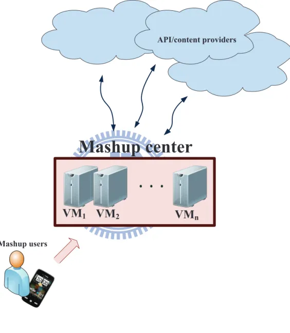
In some mobile applications, a mashup center can integrate multi-cloud servers and deliver a new service. Fig. 1.1 illustrates a mashup system that provides personalized ser-vices and adjusts the required resources (i.e., virtual machines, VMs) connected to multiple clouds. Clearly, one of the challenging issues is how to appropriately adjust the number of VMs to satisfy the quality of service (QoS) requirements for customers and minimize the

(18)

requested resources for the service provider simultaneously.

1.2 Problem and Solution

In the literature, few analytical models for cloud computing has been reported [1,2]. In [1], the authors applied queueing theory to analyze the performance tradeoff of cloud comput-ing among the maximum number of served users, the minimal resources, and the highest level of services. In [2], a non-preemptive priority queueing model was proposed to analyze the maximum profits for both users and cloud computing service providers. Nevertheless, these methods did not address the delay issue for a mashup multi-cloud system. In [3], the authors proposed a mashup architecture for the cloud-based service and use simulations to measure the delay performance of mashup clouds. In [4], a peer-to-peer mushup archi-tecture was introduced. However, to our best knowledge, the analytical model for mashup multi-cloud system has not been seen in the literature yet. The key challenge lies in the fact that the resources used in cloud computing are scalable and dynamic, including the number of virtual machines in the mashup center connected to multiple distributed cloud servers.

In this thesis, we propose an queueing theoretical model to analyze the delay per-formance of a mashup multi-cloud system, consisting of the mashup center, mobile users, and multiple cloud servers. The mashup center is responsible for adjusting the necessary resources for supporting the requested services by users. Our goal is to investigate how to analyze and determine the necessary number the servers in the mashup center to satisfy the QoS requirement according to the various users service request rate.

1.3 Thesis Outline

In this thesis, we investigate how to analyze the time delay in the mashup multi-cloud system. We provide simulation results to prove the accuracy of our model. Chapter 2

(19)

įġįġį

VM

1

VM

2

VM

n

Mashup center

API/content providers

Mashup users

Figure 1.1: An illustrative example for the service mashup model.

(20)

introduces the background of cloud computing, mashup system, queueing theory, and our developed group LBS (called JOIN). Chapter 3 shows the system model of the mashup system for two different kinds traffic. Chapter 4 analyzes the queueing model of the mashup system for the single-class traffic and two-class traffic. Chapter 5 discusses the analytical results and simulation results for the single-class traffic and two-class traffic in the mashup system. Chapter 6 gives some concluding remarks.

(21)

5

CHAPTER 2 Background

2.1 Application Services with Cloud Computing

2.1.1 Cloud Computing

In recent years, cloud computing has become very popular in academia and industry [3], [5–10]. From the business aspect, because many businesses do not always requires a lot of computing and storage, it is quite wasteful to buy a lot of servers just for a few hours. Therefore, in order to reduce the costs, they can rent a number of servers required from the cloud with certain time. That is one of the most important features for cloud computing, i.e. pay as you use. On the other side, there are many kinds of research worth in cloud computing, such as privacy [11] and time delay [1], [2]. It is worthwhile in exploring to what extent the performance can be improved when we upload the complex calculations or large data to the cloud server.

(22)

2.1.2 Mobile Service Integrated Cloud Service

More and more online applications are designed for the mobile phones due to the smart-phones are pervasive in these years [12], [13]. The mobile users usually do not know where the online applications come from. Therefore, we call these services as cloud services. Be-cause of the limits of the battery energy, storage and computing ability, we usually store or calculate the data in the cloud by uploading data to the servers [14]. For this reason, the service rate of cloud server and the number of VMs in the cloud are quite important pa-rameters. To provide a satisfying QoS to mobile users, it is important to design the mashup multi-cloud system.

2.2 Mashup System

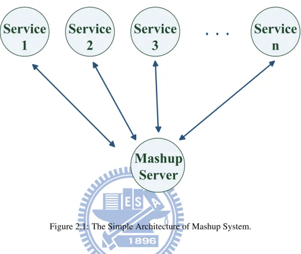
In some applications, the mashup center can integrate multi-cloud servers and deliver a new service to the mobile users or web users a personal service, just like [3], [4], [15], [16]. As shown in Fig. 2.1, depending on personal requirement, the users ask for the desired service to the mashup server which provides diversified services. Then, the mashup server requests the related server for the required resources. How to appropriately adjust the mashup server resources to satisfy the users QoS requirements and save the resources of the center server simultaneously is a challenging issue.

2.3 Queueing Theory

Queueing theorem is a mathematical method that can analyze the practical system per-formance [17], [18]. No matter what the distribution of the system flow is, the queueing theorem can be used to analyze the basic system performance. So far, there are many re-searchers using this mathematical theory to analyze various schemes. Hence, we need to

(23)

Service

1 Service

2 Service

3 Service

n

Mashup

Server

įġįġį

Figure 2.1: The Simple Architecture of Mashup System.

understand the fundamental models in queueing theorem for the reason that we want to observe the performance of the mashup multi-cloud system.

2.3.1 Overview of M/M/1 Queueing Model

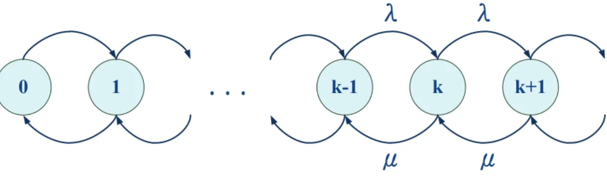
M/M/1 queue is a queueing system that the arrival customers depend on a Poisson process and are served by one server whose service time is exponential distribution. Besides, the basic service discipline is first-in-first-out. Since the arrival rate and the service rate are independent of the number of customers in the system, it is a state-independent system. As shown in Fig. 2.2, each state means the number of customers in the system. If the number of customers in the system from k to (k-1), it is implied that there is one served customer

(24)

0

1 k-1

k

k+1

ȫ

Ȫ

įġįġį

Figure 2.2: M/M/1 flow balance between states.

leaves the system. Similarly, if the number of customers in the system from (k+1) to k, it means that there is one customer enters the system. Let λ be the arrival rate to the system and µ be the service rate of the server. According to a birth-death process, we can get

λPk−1+ µPk+1= µPk+ λPk and

λP0 = µP1 ,

where Pkis the probability of having k users in the system. We calculate it by iteration and can get Pk = ( λ µ) k_P 0 . (2.1) We also know ∞ ∑ i=0 Pi = 1 . (2.2)

From (2.1) and (2.2), we can obtain

(25)

and

Pk = (1− ρ)ρk , (2.4)

where ρ = λ_µ . Therefore, the average number of customers in the system can be expressed as N = ∞ ∑ i=0 iPi = ∞ ∑ i=0 i(1− ρ)ρi = ρ 1− ρ . (2.5)

Finally, according to Littles theorem, we can express the average waiting time of the system as

W = N

λ =

1

µ− λ . (2.6)

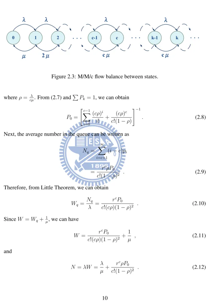
2.3.2 Overview of the M/M/c Queueing Model

The M/M/c queue is a queueing system that the customers arrive depend on a Poisson process and are served by multi-server whose service time is exponential distribution. As shown in Fig. 2.3, when the number of customers in the system (k) is more than the servers number (c), the service rate of the system is cµ. On the contrary, if the number of customers is smaller than the servers number, the service rate is kµ. Using the concept of local balance, we can express with the following:

kµPk = λPk−1 ,for k ≤ c ;

cµPk = λPk−1 ,for k ≥ c . Using literation, we can obtain

Pk=    (cρ)k k! P0 , for k ≤ c cc_ρk c! P0 , for k≥ c , (2.7) 9

(26)

0 1 c-1 c c_ȫ Ȫ

įġįġį

k-1 k c_ȫ Ȫ Ȫ 2

įġįġį

Ȫ ȫ 2_ȫ

Figure 2.3: M/M/c flow balance between states.

where ρ = _cµλ. From (2.7) and∑Pk= 1, we can obtain

P0 = [_c₋₁ ∑ i=0 (cρ)i i! + (cρ)c c!(1− ρ) ]−1 . (2.8)

Next, the average number in the queue can be written as

Nq = ∞ ∑ i=c+1 (i− c)pi = r c_ρP 0 c!(1− ρ)2 . (2.9)

Therefore, from Little Theorem, we can obtain

Wq = Nq λ = rc_P 0 c!(cρ)(1− ρ)2 . (2.10)

Since W = Wq+ 1_µ, we can have

W = r c_P 0 c!(cρ)(1− ρ)2 + 1 µ , (2.11) and N = λW = λ µ+ rcρP0 c!(1− ρ)2 . (2.12)

(27)

2.3.3 Overview of the Non-preemptive Priority Queueing Model

The queue which divides customers into multi-priority queues is called priority queue. If the higher priority customers will cut in front of the lower priority customers at the queue but will not interrupt someone who is being served in the server, it is called non-preemptive priority queue. We can express the average waiting time of i-priority customers as

W_q(i) = i ∑ k=1 E[Sk] + i−1 ∑ k=1 E[S_k′] + E[S0] , (2.13)

where E[Sk] is the average serving time of the higher priority or the same priority customers who are waiting at the queue when a i-priority customer enters the system, E[S_k′] is the average serving time of the higher priority customers, who enter the system, when a i-priority customer waits in the queue, and E[S0] is the average residual serving time of the customers who are being served by the servers when i-priority customer server.

Referring to [17], we can obtain

W_q(i) = E[S0] (1− σi−1)(1− σi) = [c!(1− ρ)(cµ) ∑c−1 n=0 (cρ)n−c n! + cµ]−1 (1− σi−1)(1− σi) , (2.14)

where σi=∑i_k=1ρk . Thus, the average waiting time in the queue can be written as

Wq = j ∑ i=1 γi γW (i) q , (2.15)

where j is the number of the customers classes. Then, the average waiting time in the system can be expressed as

W = Wq+ 1

µ , (2.16)

(28)

2.3.4 Jackson Queueing Network

Jackson Queueing Network is a network of n M/M/c queueing system with state-independent. There are some characteristic which are referred in [18]:

1. The service discipline is FIFO at all queues.

2. All external arrival rate to the node i is Poisson distribution.

3. The service times are all exponential distribution with mean µiat node i. 4. The service times are independent with the other nodes.

5. A customer completing service at node i will either go to node j with a probability Pij or leave the system at node i with probability 1−∑n_j=1Pij.

6. At each node i, the queue capacity is infinite.

Therefore, we can make good use of the Jacksons network theorem to analyze the system performance of our network if the system meets the above conditions.

2.4 Literature Survey

There are several researches to discuss the issue of the mashup service and the cloud com-puting service in the recent years. They are briefly introduced as follows:

2.4.1 Performance Analyzing of the Cloud Services

An Optimistic Differentiated Service Job Scheduling System for Cloud Computing Service Users and Providers [2]

In [2], a non-preemptive priority M/G/1 queueing model is proposed to analyze the differ-ential QoS requirements of users who use the cloud computing resources. Then, the cloud services provider supply the resources to the users for the purposes to satisfy the QoS of the users with different requirements. Moreover, the author builds a cost function to get the

(29)

approximate optimal value of service for each job in the non-preemptive priority M/G/1 queueing model.

Because cloud computing is a new computing technique, this paper partition the users requirement of QoS into several classes and use queueing theorem to model the sys-tem for job scheduling. The author regards the cloud server as a large server that can provide different service rate according to users requirements. Then, the mathematical analysis can compute the optimistic solution that can not only guarantee the QoS require-ments of the cloud computing users jobs, but also can gain the maximum profits for the cloud computing service provider.

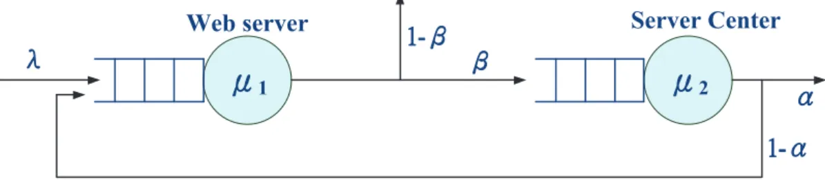
Service Performance and Analysis in Cloud Computing [1]

In [1], the authors studied the computer service performance in cloud computing by propos-ing a queuepropos-ing network model, composed of a Web server and a service center, as shown in Fig. 2.4. Then, each regard as an integral component that is modeled as a single queue. The author considers that upon completion the service at the web service, the customer leaves the system with the probability 1− β, or enters the service center with the probability β. Besides, after a customer is completed the service by the service center, it returns to the web server with probability 1− α, or exits the system with the probability α. By using this model, the author develops an approximation method for computing the Laplace transform of a response time distribution in the cloud computing system. Hence, the relationship among the maximum number of customers, the minimum service resources and the highest level of services is found in this approach and the numerical experiments had conducted to prove the approximate method is feasible.

(30)

ȫ1

ȫ2

Web server Server Center

ȡġ ĲĮȡġ

Ƞġ ĲĮȠġ Ȫġ

Figure 2.4: The queueing model for computer service in cloud computing.

2.4.2 Mashup Service Integrating the Cloud Services

Towards Cloud Oriented Service MashUp [3]

In [3], the authors proposed a cloud-oriented service mashup system with the advantages of the cloud, grid, web services and other technologies. In addition, during the procedure of mashup service to meet the multi-kinds of service applications, the service information interaction, classification and process is supported. The architecture of the mashup service is shown in Fig. 2.5. The web site integrates the service which is Yahoo and Amazon to provide a diversified service to the client. Then, the end-users can use various services resources and add the widgets to their personal service application space so that they can build their customized services based on their own requests.

The authors built a mashup service system to provide an easy tool and a generally unified appearance. The response time in the server side was tested and compared with iGoogle platform.

2.4.3 Summary

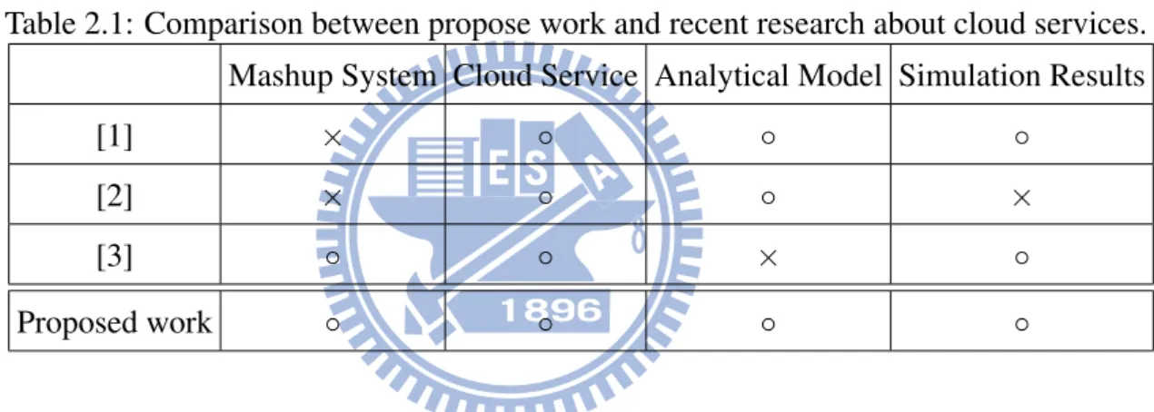
Comparing these researches about the performance of cloud services, we can find that the time delay of the mashup multi-cloud system is an important issue but has not investigated.

(31)

Client

Browser

Web Site

Amazon

Yahoo!

Mashup

Figure 2.5: The architecture of the mashup service.

Table 2.1: Comparison between propose work and recent research about cloud services. Mashup System Cloud Service Analytical Model Simulation Results

[1] × ◦ ◦ ◦

[2] × ◦ ◦ ×

[3] ◦ ◦ × ◦

Proposed work ◦ ◦ ◦ ◦

Therefore, we propose a queueing network to model a mashup system to satisfy the QoS requirements of users. Comparison table is shown in Table 2.1. Furthermore, performance analysis and simulation results will be introduced in remaining chapters.

2.5 JOIN Project

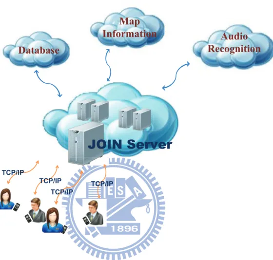
JOIN is an application that we can invite friends who have the same interests [19]. The persons who are invited can vote that which place and time they wanted. The architecture of JOIN is shown in Fig. 2.6. During the JOIN service execution duration, there are four steps.

(32)

TCP/IP TCP/IP TCP/IP TCP/IP

JOIN Server

Database

Map

Information

_Audio

Recognition

Figure 2.6: The Architecture of JOIN System

(1) Firstly, once JOIN users login the server and execute the JOIN by choosing the interest-ing groups via the interface on the handsets, they are able to exchange the information with others who in the same group by JOIN server. During this stage, JOIN server will connects to the cloud database server to obtain the information.

(2) Secondly, JOIN server provides the surrounding information (includes businesses and friends) to the users who execute JOIN. During this stage, JOIN server will connects to the cloud database server to obtain the locations of the same interesting friends and connects

(33)

to the cloud map information server to obtain the locations of the surrounding businesses. (3) The user who receives the information from JOIN server can hold the activity by invit-ing the friends, choosinvit-ing one destination and proposinvit-ing the options of the datinvit-ing time. Once JOIN server receives the information about holding activity, the arranged meeting location and time will be sent to the corresponding users. During this stage, the user might use the audio recognition for ease to use when holding the activity. At that time, the user connected to the cloud audio recognition server through JOIN server.

(4) After voting, the users who are invited will return their preferred dating time to JOIN server. Next JOIN server will collects the data from each user, and sends the final statistics of the vote to all the invited users. This step also stores the result of the activity in the cloud database.

JOIN server is just like a mashup center which integrates the database server, map information server and audio recognition server to provide the users a location-based ser-vice. The service aims to provide the users a real-time location-based service, so the time delay of the service is very important.

(34)

18

CHAPTER 3 System Model and Problem Formulation

3.1 System Model

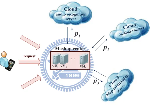
In fact, there are abundant and versatile cloud resources in the Internet, such as Google apps, Youtube, Hotmail, etc. Therefore, many cloud applications developers utilize cloud resources of other companies to create their own new applications. As shown in Fig. 3.1, a mashup cloud service architecture consists of mobile users, mashup center and multi-cloud servers. We consider the multi-cloud servers of database, map information, and audio recognition. Denote P1, P2 and P3 as the probabilities of the mashup center requesting to the server of audio recognition, database, and map information, respectively. According to the architecture in Fig. 3.1, we propose a corresponding queuing model for the mashup multi-cloud servers with single- and two-class traffic loads.

3.1.1 Single-Class Traffic Case

To begin with, we first introduce the queueing model for the mashup cloud system in sup-porting the single-class traffic, as shown in Fig. 3.2. The mashup center is composed of

(35)

įġįġį

VM1 VM2 VMn Mashup center request Cloud audio recognition server 1

p

databCloudase se rver 2

p

Clo ud Map infor mat ion serve r 3

p

Figure 3.1: A Simple Example of Mashup System.

(36)

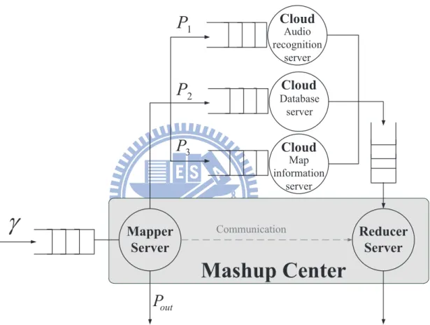
mapper server and reducer sever. When a request enters the mapper server, the service request will be forwarded to audio recognition, database, and map information with prob-ability P1, P2, and P3, respectively. Also, if the service does not require the cloud server, the traffic will leave the mashup system with a probability of Pout. The reducer server will integrate the outcomes of the service request to the servers of database, map information or audio recognition, and then respond the integrated results to the customers.

In Fig.3.2, the mapper server and reducer server are modeled as the M/M/c queue, whereas the database server, map information server and audio recognition server are mod-eled as an M/M/1 queue. We consider the first in first out (FIFO) queue discipline, Poisson distributed arrival process, and the exponential distributed service time for all the servers, including mapper, reducer, database, map information and audio recognition.

3.1.2 Two-Class Traffic Case

Next we consider a two-class traffic case in the mashup system. We classify the users (payers and free users) into two groups. The payers have higher priority to be served than the free users. When a payer asks the service from the mashup system, it will be placed in front of free users, and follow the FIFO queueing discipline for customers with the same class users. When a free user asks for the service, it will line up at the end of the queue if another user is waiting for serving. The service request will enter into the cloud servers or leave the system with the probability P1, P2, P3, and Poutmentioned before. In addition, we also assume that the mapper server and reducer server are modeled as M/M/c queues. Similarly, database server, map information server and audio recognition server are modeled as M/M/1 queue. The arrival rate of the high priority request and the low priority request is Poisson distribution. The service time at the servers are all exponentially distributed.

(37)

Mapper

Server

Reducer

Server

Communication

g

1

P

2

P

3

P

out

P

Mashup Center

Cloud

Database server

Cloud

Audio recognition server

Cloud

Map information server

Figure 3.2: Queueing Model of Mashup System for Single-Class Traffic.

(38)

Non-Preemptive Priority Service Discipline Only in Mapper Server

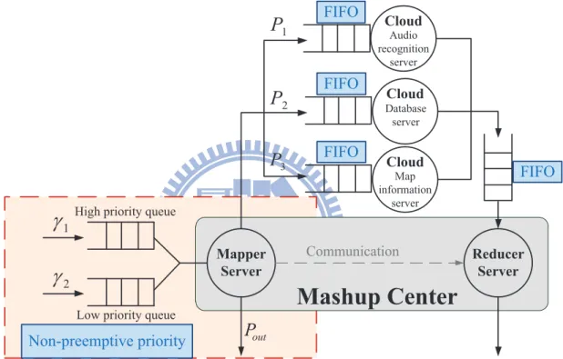
In the condition that only service discipline of mapper server is non-preemptive priority, we assume all the requests which are served by mapper server following non-preemptive priority rule and let all the requests entering the cloud servers be treated as the same class. Hence, we change the queueing model from Fig. 3.2 to Fig. 3.3. We divide the external arrival into two classes. The high priority users is payers. The low priority users is free users. In Fig. 3.3, the service of mapper server discipline is non-preemptive priority and the others discipline is FIFO.

Non-Preemptive Priority Service Discipline in Mashup System

In the condition that all the services in mashup system are non-preemptive priority, we change the queueing model from Fig. 3.2 to Fig. 3.4. There are two kinds of external arrival, payers and free users. When a request of the payer enter mashup system, it will be placed in front of free users, and follow the FIFO queueing discipline for customers with the same class users. When a free user asks for the service, it will line up at the end of the queue if another user is waiting for serving. The service discipline in all the servers of mashup system will follow the rule describing above.

3.2 Problem Formulation

In the mashup system, how to adjust the number of VMs appropriately to satisfy the QoS requirement is a crucial issue. Because the arrival rate of the application service request is not always the same, it is important to investigate how to provide a satisfying QoS to users and do not waste system resources simultaneously. System time is defined as the duration from the beginning when a service is requested until it leaves the mashup system. Because the server may be congested due to high arrival rates, increasing the number of VMs can

(39)

Mapper Server Reducer Server Communication 1

g

1

P

2

P

3

P

out

P

Mashup Center

Cloud Database server Cloud Audio recognition server Cloud Map information server 2

g

High priority queue

Low priority queue

Non-preemptive priority

FIFO FIFO

FIFO

Figure 3.3: Queueing Model of Mashup System for Two-Class Traffic with Non-preemptive Priority Service Discipline in Mapper Server Only.

(40)

g

1

P

2

P

3

P

out

P

Mashup Center

g

High priority queue

Low priority queue

Non-preemptive

priority

Figure 3.4: Queueing Model of Mashup System for Two-Class Traffic with All Non-preemptive Priority Service Discipline.

(41)

reduce the average system time within certain threshold.

3.2.1 Single-Class Traffic Case

In the case with only one single-class traffic, we discuss the effects of arrival rates on the average system time under various arrival rates for requesting cloud services and the service time of cloud servers. Specifically, we predict how many VMs are needed at the mashup center for different situations. Because high request rates for cloud services lead to high arrival rates to the reducer server, the request rate for the cloud services will affect how many VMs are needed at the reducer servers. If the service time of the cloud server is long and the request rate for cloud servers is high, we can expect that the cloud servers will be very busy. Therefore, we only discuss the condition that the service rate of cloud server is slow and the request rate for cloud servers is low.

3.2.2 Two-Class Traffic Case

In the case with two-class traffic, we discuss how to provide differentiated QoS to the payers and free users. The total arrival rate is the sum of the arrival rates of the high priority users and the low priority users. Provided that we know the proportion of the high priority arrival rate to the total arrival rate, we formulate a problem to calculate the number of the required VMs subject to the QoS constraint of the priority user.

(42)

26

CHAPTER 4 Performance Analysis of Mashup

Services

In this chapter, we use queueing theory to analyze the average waiting time of the mashup system. In the following, we will investigate how to obtain the average waiting time in the single-class traffic queue and two-class traffic queue.

4.1 System Time Analysis With Single-Class Traffic

Based on the queueing model we mentioned in Section 3.1.1, we can apply Jackson net-work’s theorem to the mashup multi-cloud system. According to Jackson netnet-work’s theory, the joint probability mass function for the number of customers (n) in a network with M queues is written as

P (en) = P (n1, n2, ..., nM)

(43)

where ni is the number of customers in the i-th queue, and Pi(ni) is the probability of having ni users in the i-th queue (i = 1,· · · , M). Let γ be the total arrival rate. Denote the arrival rates to the mapper server, reducer server, audio recognition server, database server, and map information server as λm, λr, λ1, λ2, and λ3, respectively. Also, denote the service rate of the mapper server, reducer server, audio recognition server, database server, and map information server as µm, µr, µ1, µ2, and µ3 Then, we can calculate the arrival rates at each server as follows:

λm = γ ;

λ1 = P1γ ; λ2 = P2γ ; λ3 = P3γ ;

λr = (P1+ P2+ P3)γ . (4.2)

where P1, P2, and P3denote the probabilities of the service request will enter into the audio recognition server, database server, and map information server. Denote Pm0and Pr0as the probability of zero customer in the mapper server and reducer server, respectively, and Let

m and r be the number of VMs in the mapper server and reducer server. Substituting the

average number in the M/M/1 queuing system (2.5), and the average number in the M/M/c queuing system (2.12), into (4.1). Then, we can obtain

Pnm,n1,n2,n3,nr = [ rmnm a(nm) Pm0 ] [∏3 i=1 ρni i (1− ρi) ] [ rrnr a(nr) Pr0 ] , (4.3) where ρi = λi µi ; ρm = λm mµm ; 27

(44)

ρr = λr rµr ; rm = λm µm ; rr= λr µr ; a(nm) =    nm! , for nm < m mnm−m_{m! , for n} m ≥ m ; a(nr) =    nr! , for nr < r rnr−r_{r! , for n} r ≥ r ; Pm0= [_m₋₁ ∑ k=0 (mρm)k k! + (mρm)m m!(1− ρm) ]−1 ; Pr0 = [_r₋₁ ∑ k=0 (rρr)k k! + (rρr)r r!(1− ρr) ]−1 ; (4.4) The average number of service requests in the mashup system is the sum of the average service requests in all the servers, including mapper, reducer, audio recognition, database, and map information. Then, the average number of the service requests in the mapper server and reducer server can be written as

Nm = rm+ [ rm+1m /m m!(1−ρm)2 ] Pm0 , (4.5) and Nr = rr+ [ rrr+1/r r!(1−ρr)2 ] Pr0 . (4.6)

(45)

The average number of requests to the cloud server is

Ni =

ρi 1− ρi

i = 1, 2, 3 . (4.7)

To sum of (4.5), (4.6) and (4.7) , the average number of the requests in the mashup system can be written as N = Nm+ 3 ∑ i=1 Ni+ Nr. (4.8)

According to Little’s theorem, we can express the average waiting time of the mashup system as

W = N

γ . (4.9)

In summary, from (4.9), we can evaluate the performance of our framework. We will prove that our mathematical analysis result is appropriate by comparing with the sim-ulation result in the next chapter.

4.2 System Time Analysis With Two-Class Traffic

4.2.1 Non-Preemptive Priority Service Discipline Only in Mapper

Server

Based on the queueing model we described in Fig. 3.3, we can use queueing theory to analyze the average waiting in the mashup system with two-class traffic. As shown in Fig. 3.3, we cannot use the theory of Jackson network in this model because FIFO is not the only service discipline in all queues. Therefore, we divide the system into two systems, as shown in Fig. 4.1. System 1 consists of the mapper server, and System 2 is composed of the database server, map information server, audio recognition server and reducer server.

(46)

g

1

P

2

P

3

P

out

P

Mashup Center

g

High priority queue

Low priority queue

Non-preemptive priority FIFO FIFO FIFO FIFO

System 1

System 2

(47)

Clearly, systems 1 and 2 can be viewed as a serial queue. Beause system 1 is a non-preemptive priority queue, the average waiting time of the i-priority users in the queue becomes W_qm(i) = [c!(1− ρ)(cµ) ∑c−1 n=0 (cρ)n−c n! + cµ]−1 (1− σi−1)(1− σi) , (4.10) where σi= ∑i

k=1ρk . Thus, the average waiting time in the queue for all the users can be expressed as Wqm = 2 ∑ i=1 γi γW (i) qm , (4.11)

where γ₁and γ₂ are the arrival rates of the high priority users and low priority users, respec-tively. Denote γ=γ1+γ2 as the arrival rate of all the users. Then we can obtain the average

waiting time for the high priority users in system 1 as

W_s1(1) = W_qm(1)+ 1

µm

. (4.12)

Furthermore, the average waiting time for the low priority users in system 1 is equal to

W_s1(2) = W_qm(2)+ 1

µm

. (4.13)

Because the service discipline of all the servers in system 2 is FIFO, system 2 can be viewed as a Jackson’s network. From (4.6) and (4.7), we can get the average number of the service requests in system 2 as follows:

Ns2= 3 ∑

i=1

Ni+ Nr . (4.14)

According to Little’s theorem, we can get the average waiting time of system 2

Ws2 =

Ns2

γ(P1+ P2+ P3)

. (4.15)

(48)

Because the probability of the requests entering system 2 is 1− Pout, the average waiting time of the high priority users in the mashup system can be expressed as

W(1) = W_s1(1)+ (1− Pout)Ws2 , (4.16) and the average waiting time of the low priority users in the mashup system is equal to

W(2) = W_s1(2)+ (1− Pout)Ws2 . (4.17) In summary, by getting (4.16) and (4.17), we can evaluate the performance of our framework. In the next chapter, we will prove that our mathematical analysis result is appropriate by comparing with the simulation result.

4.2.2 Non-Preemptive Priority Service Discipline in Mashup System

According to the queueing model we described in Fig. 3.4, first we calculate the average waiting time of mapper server, reducer server, database server, map information server, and audio recognition server, respectively. Then, times the corresponding probability and sum will get the average waiting time of mashup system. From (4.10), we can obtain the average waiting time of the i-priority users in the queue of mapper server, reducer server, and cloud server as

W_qm(i) = [m!(1− ρm)(mµm) ∑m₋₁ n=0 (mρm)n−m n! + mµm]−1 (1− σmi−1)(1− σmi) , (4.18) W_qr(i) = [r!(1− ρr)(rµr) ∑r₋₁ n=0 (rρr)n−r n! + rµr]−1 (1− σri−1)(1− σri) , (4.19) W_qj(i) = µj −1_ρ j (1− σji−1)(1− σji) , j = 1, 2, 3. (4.20)

(49)

Then, the average waiting time of the high priority users in the mapper server, reducer server, and cloud servers can be expressed as

W_m(1) = W_qm(1)+ 1 µm , (4.21) W_r(1) = W_qr(1)+ 1 µr , (4.22) W_j(1) = W_qj(1)+ 1 µj , j = 1, 2, 3. (4.23)

and the average waiting time of the low priority users in the mapper server, reducer server, and cloud servers can be written as

W_m(2) = W_qm(2)+ 1 µm , (4.24) W_r(2) = W_qr(2)+ 1 µr , (4.25) W_j(2) = W_qj(2)+ 1 µj , j = 1, 2, 3. (4.26)

Because the probability of the requests entering audio recognition server, database server, and map information server is P1, P2, and P3, respectively, and the probability of the re-quests entering reducer server is (P1+P2+P3), the average waiting time of the high priority users in the mashup system is

W(1) = W_m(1)+ P1W (1) 1 + P2W (1) 2 + P3W (1) 3 + (P1+ P2+ P3)Wr(1) , (4.27) and the average waiting time of the low priority users in the mashup system is

W(2) = W_m(2)+ P1W1(2)+ P2W2(2)+ P3W3(2)+ (P1+ P2+ P3)Wr(2) . (4.28)

(50)

34

CHAPTER 5 Numerical Results

5.1 Single-Class Traffic Case

We fist discuss the effects of the arrival rate on the average waiting time in the mashup system. In the single-class traffic loads, we discuss three different cases, including high request rate to the cloud server, low request rate to the cloud server, and low service rate of cloud server. In the following subsections, the average waiting time was evaluated accord-ing to (4.9) for various arrival rate. As shown in Figs. 5.1 - 5.4, this analysis method can compute the average waiting time for the mashup system. The discrepancy is due to the limitation on the simulation number of service requests.

5.1.1 Effects of Number of VMs in the Mashup Center on Overall

System Time With High Request Rate to the Cloud Servers

In this case, we give the initial parameters of the mashup system in Table 5.1. We assume that the request rate for the cloud services is high. That is, the probability of entering the cloud servers from the mapper server (i.e. 1− Pout) is 0.75. The probability of the mashup

(51)

center requesting to the server of database, map information, and audio recognition are 0.2, 0.5, and 0.05, respectively. Under different number of VMs in the mapper server and reducer server, we investigate the effect of the arrival rate, which the region is from 1 request/sec to 25 requests/sec, on the average waiting time of mashup system.

Figs. 5.1 and 5.2 show the relation between the average waiting time and the arrival rates for one VM and two VMs in the reducer server, respectively. Clearly, the average waiting time of mashup system increases as the arrival rate increases. From Fig. 5.1, the average waiting time increases sharply at nine request/sec with one VM at the mapper server, and 13 request/sec with two or three VMs at the mapper server. Nevertheless, if the reducer server can have two VMs, the breaking point of waiting time can be extended to 19 request/sec with two VMs in the mapper server as seen in Fig. 5.2. Note that the increase of VM in the reducer servers is also important for reducing the waiting time. Without the enough number of VMs at the reducer server, the increase of VM at the mapper server is not very useful as compared the cases of three VMs in Fig. 5.1 and Fig. 5.2. Therefore, our results suggest that we need to appropriately adjust the number of VMs in the mapper server and reducer server to shorten the waiting time to guarantee the QoS for the mashup multi-cloud system.

5.1.2 Effects of Number of VMs in the Mashup Center on Overall

System Time With Low Request Rate to the Cloud Servers

In this case, we give the initial parameters of the mashup system in Table 5.2. We assume that the request rate for the cloud services is low. That is, the probability of entering the cloud servers from the mapper server (i.e. 1− Pout) is 0.25. The probability of the mashup center requesting to the server of database, map information, and audio recognition are 0.09, 0.15, and 0.01, respectively. Under different number of VMs in the mapper server and reducer server, we investigate the effect of the arrival rate, which the region is from 1

(52)

Table 5.1: Simulation Parameters for Mashup System With High Request Rate for Cloud Services - Case I

Parameter Value

External arrival rate (γ) [1:25] request/sec Service rate of the mapper server (µm) 10 request/sec

Service rate of the reducer server (µr) 10 request/sec Service rate of the database server (µ1) 50 request/sec Service rate of the map information server (µ2) 50 request/sec Service rate of the audio recognition server (µ3) 50 request/sec

The probability that will leave the system

from the mapper server (Pout) 0.25

The probability that will enter the database

server from the mapper server (P2) 0.2

The probability that will enter the map information

The probability that will enter the audio recognition

(53)

5 10 15 20 25 0 1 2 3 4 5 6 7 8 9 10

Arrival rate (request/sec)

Average waiting time (sec)

Anl,m=1 Anl,m=2 Anl,m=3 Sim,m=1 Sim,m=2 Sim,m=3

Figure 5.1: Effect of the arrival rate on the average waiting time of mashup system with one VM in the reducer server for case I.

(54)

5 10 15 20 25 0 1 2 3 4 5 6 7 8 9 10

Figure 5.2: Effect of the arrival rate on the average waiting time of mashup system under two reducer servers situation for case I.

(55)

request/sec to 25 requests/sec, on the average waiting time of mashup system.

Fig. 5.3 shows the effects of arrival rates on the average waiting time in the case of having one VM in the reducer server and has lower request rate for cloud servers (Pout = 0.75). As shown in Fig. 5.3, the average waiting time increases sharply when γ = 9 requests/sec and m = 1, which is the same as Fig. 5.1. Because the rate of requesting cloud services 1− Pout = 0.25 in Fig. 5.3 is smaller than 1− Pout = 0.75 in Fig. 5.1, the break point of sharp waiting time will be extended to γ = 19 requests/sec from γ = 13 requests/sec in the case of m = 2. One can see that for m = 3 the break point of waiting time is larger than γ = 25 requests/sec in Fig. 5.3, which is much higher than the breaking point γ = 13 requests/sec in Fig. 5.1. Thus, in the case of low request rate for cloud servers, our results imply that we only need to appropriately adjust the number of VMs in the mapper server to guarantee the QoS for the mashup multi-cloud system.

5.1.3 Effects of Number of VMs in the Mashup Center on Overall

System Time With Low Service Rate of Cloud Servers

In this case, we give the initial parameters of mashup system in Table 5.3. Note that the service rates of all servers, including mapper, reducer, database, map information, and audio recognition, are obtained from our developed mobile cloud service application, called JOIN [19]. Under the different number of VMs in the mapper server, we investigate the effect of the arrival rate, which the region is from 1 request/sec to 23 request/sec, on the average waiting time of mashup system.

Comparing Fig. 5.3 with Fig. 5.4, one can observe the effect of various service rates of cloud servers on the average waiting time. Specifically, as compared to µ1 = µ2 = µ3 = 50 in Case II, the slower service rates of µ1 = 2, µ2 = 4.5, µ3 = 0.38 in Case III lead to the earlier breaking point γ = 22 requests/sec in the case of m = 3. Therefore, when the delay performance is already restrained by the service rate of cloud servers, the increase of

(56)

Table 5.2: Simulation Parameters for Mashup System With Low Request Rate for Cloud Services - Case II

Parameter Value

External arrival rate (γ) [1:25] request/sec Service rate of the mapper server (µm) 10 request/sec

Service rate of the reducer server (µr) 10 request/sec Service rate of the database server (µ1) 50 request/sec Service rate of the map information server (µ2) 50 request/sec Service rate of the audio recognition server (µ3) 50 request/sec

(57)

5 10 15 20 25 0 1 2 3 4 5 6 7 8 9 10

Figure 5.3: Effect of the arrival rate on the average waiting time of mashup system with one VM in the reducer server for case II.

(58)

Table 5.3: Simulation Parameters for Mashup System With Low Service Rate of Cloud Servers - Case III

Parameter Value

External arrival rate (γ) [1:23] request/sec Service rate of the mapper server (µm) 9.375 request/sec Service rate of the reducer server (µr) 8.131 request/sec Service rate of the database server (µ2) 2.066 request/sec Service rate of the map information server (µ3) 4.5 request/sec Service rate of the audio recognition server (µ1) 0.382 request/sec

(59)

5 10 15 20 0 1 2 3 4 5 6 7 8 9 10

Figure 5.4: Effect of the arrival rate on the average waiting time of the mashup system with one VM in the reducer server for case III.

the number of VMs will not improve the delay performance, and thus the suitable number of VMs in the mapper server can be determined.

5.2 Two-Class Traffic Case

We consider that there are two different priorities users entering the mashup multi-cloud system. We discuss the effect of the ratio of high-priority request rate to the total request rate (ph) on the average waiting time of high or low priority users. Section 5.2.1 discuss

(60)

how to guarantee the QoS of the high-priority users for various arrival rate and p_h. In Section 5.2.2, we discuss how to guarantee the QoS of the low-priority users for various arrival rate and p_h.

In the following subsections, the average waiting time of high and low priority users were evaluated according to (4.16) , (4.17), (4.27), and (4.28). As shown in Figs. 5.5, 5.6, 5.7, 5.10, 5.11, and 5.12, this analysis method can compute the average waiting time for the mashup system. The little inaccuracy may be caused by limitation simulation number of service requests. In our simulation, we adopt the parameters of Section 5.1.3, as shown in the Table 5.3. Under different value of p_h, we investigate the effect of the arrival rate, which the region is from 1 to 23, on the average waiting time for high and low priority users in the mashup system.

5.2.1 Effects of p

h

on the Overall System Time of High Priority Users

The Service in Mapper Server is Non-Preemptive Priority and Other Services are FIFO

Figures 5.5, 5.6 and 5.7 show the effect of m and γ to the average waiting time of high priority users in the mashup system with p_h = 0.1, p_h = 0.5 and p_h = 0.9, respectively. In Fig. 5.5, increasing the mapper servers will not change the average waiting time because the high priority requests rate is low. In this case, the high service requests will get the fast response from the mapper server. Besides, the average waiting time increases sharply at 22 requests/sec because of low service rate of cloud servers. However, the breaking point of waiting time can be changed to 18 requests/sec in the case of m = 1 when p_h = 0.5 as seen in Fig. 5.6. From Fig. 5.7, when ph = 0.9, the break point of sharp waiting time will be

changed to 10 request/sec in the case of m = 1, and 20 request/sec in the case of m = 2. Therefore, We find that it is important to adjust the number of VMs in the mapper server appropriately based on the value p_h.

(61)

5 10 15 20 0 1 2 3 4 5 6 7 8 9 10

Average waiting time of the high priority users (sec)

Figure 5.5: Effect of the arrival rate on the average waiting time of high priority users in the mashup system when only service discipline of mapper server is non-preemptive priority and ph = 0.1.

(62)

5 10 15 20 0 1 2 3 4 5 6 7 8 9 10

(63)

5 10 15 20 0 1 2 3 4 5 6 7 8 9 10

(64)

All Services in the Mashup System are Non-Preemptive Priority

Figures 5.8 and 5.9 show the effect of m and γ to the average waiting time of high priority users in the mashup system with p_h = 0.1 and p_h = 0.9, respectively. In Fig. 5.8, we find that the average waiting time of the high priority users can be improved when γ ≥ 22. In Fig. 5.9,in the case of m = 3, the average waiting time also decreased when γ ≥ 22. Therefore, when all the service discipline in the mashup system is non-preemptive priority, the performance of high priority users can be improved effectively.

5.2.2 Effects of p

h

on the Overall System Time of Low Priority Users

The Service in Mapper Server is Non-Preemptive Priority and Other Services are FIFO

Figures 5.10, 5.11 and 5.12 show the effect of m and γ to the average waiting time of low priority users in the mashup system with p_h = 0.1, p_h = 0.5 and p_h = 0.9, respectively. Comparing Fig. 5.10, Fig. 5.11, and Fig. 5.12, one can observe the effect of p_h on the average waiting time of low priority users. Specifically, we find that p_h will not affect the average waiting time of low priority users too much. Furthermore, from Fig. 5.5 and Fig. 5.10, if we adjust the number of VMs to guarantee the QoS of high priority users, we cannot guarantee the QoS of low priority users with p_h = 0.1. However, with p_h = 0.9, adjusting the number of VMs for the performance of high priority users can also guarantee the performance of low priority users simultaneously as seen in Fig. 5.7 and Fig. 5.12.

All Services in the Mashup System are Non-Preemptive Priority

Figures 5.13 and 5.14 show the effect of m and γ to the average waiting time of low priority users with p_h = 0.1 and p_h = 0.9, respectively. Comparing to Fig. 5.10 and Fig. 5.12, it does not change much in the average waiting time for low priority users.

(65)

5 10 15 20 0 1 2 3 4 5 6 7 8 9 10

Figure 5.8: Effect of the arrival rate on the average waiting time of high priority users in the mashup system when all service discipline is non-preemptive priority and p_h = 0.1.

(66)

5 10 15 20 0 1 2 3 4 5 6 7 8 9 10

Figure 5.9: Effect of the arrival rate on the average waiting time of high priority users in the mashup system when all service discipline is non-preemptive priority and p_h = 0.9.

(67)

5 10 15 20 0 1 2 3 4 5 6 7 8 9 10

Average waiting time of the low priority users (sec)

Figure 5.10: Effect of the arrival rate on the average waiting time of low priority users in the mashup system when only service discipline of mapper server is non-preemptive priority and ph = 0.1.

(68)

5 10 15 20 0 1 2 3 4 5 6 7 8 9 10

(69)

5 10 15 20 0 1 2 3 4 5 6 7 8 9 10

雲端運算混搭服務性能分析技術之研究

國 立 交 通 大 學

電信工程研究所

碩 士 論 文

雲端運算混搭服務性能分析技術之研究

Performance Modeling for Mashup Services in

Cloud Computing

研究生：楊媁萍

指導教授：王蒞君 教授

雲端運算混搭服務性能分析技術之研究

Performance Modeling for Mashup Services in Cloud

Computing

研 究 生：楊媁萍

Student：Wei-Ping Yang

指導教授：王蒞君 Advisor：Li-Chun Wang

國 立 交 通 大 學

電信工程研究所

碩 士 論 文

雲端運算混搭服務性能分析技術之研究

學生：楊媁萍

指導教授：王蒞君 教授

國立交通大學

電機學院電信工程研究所

摘要

近年來，雲端運算 (Cloud Computing) 結合智慧型手機的應用快

速發展。現今很多的應用結合多個雲端服務以更多樣化且方便的形

式提供給使用者。在這些應用之中，即時性是相當重要的議題，例

如以位置為基礎的服務 (Location-Based Services, LBSs)。在這篇論

文中，我們將討論一個由多個雲端服務所構成的混搭系統 (Mashup

System) 的效能分析技術。本論文提出一個利用排隊網路 (Queueing

Network) 的分析技術以評估針對在不同的服務要求，如何保證到達

使用者需要的服務品質。在此分析模組下，我們分別探討單一類別

的 要 求 (Single-Class Traffic) 和 兩 種 類 別 的 要 求 (Two-Class

Traffic) ，討論在不同的服務要求速率下，如何適當的調整混搭中心

(Mashup Center) 的虛擬伺服器 (Virtual Machine, VM) 的個數以滿

足使用者的服務品質需求。利用模擬的結果，我們證明所提出的方

法的正確性。因此，本論文所建議之以排隊理論的分析模型可以提

供一個很好的混搭多雲系統的性能分析。

Abstract

Acknowledgments

Contents

List of Tables

List of Figures

Glossary of Symbols

CHAPTER 1

Introduction

1.1

Motivations

1.2

Problem and Solution

1.3

Thesis Outline

įġįġį

VM

VM

VM

Mashup center

CHAPTER 2

Background

2.1

Application Services with Cloud Computing

2.1.1

Cloud Computing

2.1.2

Mobile Service Integrated Cloud Service

2.2

Mashup System

2.3

Queueing Theory

Service

1

Service

2

Service

3

Service

n

Mashup

Server

įġįġį

國立交通大學

碩士論文

指導教授：王蒞君教授

研究生：楊媁萍

國立交通大學

碩士論文

指導教授：王蒞君教授

的要求 (Single-Class Traffic) 和兩種類別的要求 (Two-Class

_Audio