適用於無線微型感測網路之具容錯性與攻擊抵抗性之多重路徑資訊傳送機制

全文

(1)國立交通大學資訊科學與工程研究所碩士論文. 適用於無線微型感測網路之具容錯性與攻擊抵抗性之多重路徑資訊傳送機制 A Fault-Tolerant, Attack-Resistant Multipath Information Delivery Scheme for Wireless Sensor Networks. 研究生：陳厚坤指導教授：謝續平. 中華民國. 教授. 九十五. 年六月.

(2) 適用於無線微型感測網路之具容錯性與攻擊抵抗性之多重路徑資訊傳送機制研究生：陳厚坤. 指導教授：謝續平教授. 國立交通大學資訊工程學系. 摘要對於大多數無線微型感測網路的應用而言，資訊傳輸的可信賴程度與其安全性為兩項主要的考量因素。由於感測節點通常佈建於無人照料或敵人充斥的環境中，並且感測到的資訊必須經由節點間本質即不穩定的無線連結傳輸至後端基地台，如何正確、安全且即時地傳送感測到的資訊實為一大挑戰。為了解決此項議題，我們提出了一個基於封包切割概念的多重路徑資訊傳送機制，FAMIDS。在此機制之下，資料來源節點將原始封包利用增加冗位元的方式切割成數個小封包，並且利用多重路徑安全地傳送該封包。即使部分的小封包接收錯誤，後端基地台仍能重建原始封包。除此之外，我們建立了分析 FAMIDS 所能達到的傳輸可信賴程度之分析模型。針對不同的網路條件，我們研究該分析模型之表現情形，並且提出能找出最佳封包切割方式的有效率演算法，以達到最佳的傳輸可信賴程度。相較於傳統之暴力法，我們提出之演算法能有效降低每次封包傳輸之計算複雜度。.

(3) A Fault-Tolerant, Attack-Resistant Multipath Information Delivery Scheme for Wireless Sensor Networks Student: Hou-Kun Chen Advisor: Shiuh-Pyng Shieh Department of Computer Science and Information Engineering National Chiao Tung University. Abstract Transmission reliability and information confidentiality are two of the major concerns for most applications of wireless sensor networks. Since sensor nodes are usually deployed in unattended or adversarial environments and sensed information is transmitted through inherent instable wireless links among sensor nodes to the base station, how to deliver sensed information correctly, securely and instantaneously becomes a challenging problem. To deal with this issue, we propose an enhanced multipath information delivery scheme FAMIDS based on the concept of packet splitting. With the proposed scheme, the source node splits the original data packet into several sub-packets by adding redundancy, and securely transmits the sub-packets through multiple paths. The base station can reconstruct the original data packet even if part of sub-packets is incorrectly received.. In addition, we develop an analytical model for evaluating communication reliability achieved by our scheme and study the behavior of the analytical form under different network conditions. For each network model, we propose an algorithm for finding the optimal way of packet splitting with highest communication reliability. Compared with the traditional brute-force approach, the proposed algorithms efficiently reduce the computational complexity for each packet transmission.. ii.

(4) 誌. 謝. 這份論文能夠順利完成，首先要感謝指導教授謝續平教授從大學專題以來的辛勤指導。感謝您給予了我這麼優良的研究環境以及優秀的實驗室伙伴，讓我能在每次熱烈的討論當中茁壯與成長。感謝楊明豪教授與黃育綸教授在論文撰寫過程當中提供寶貴的指導與建議。碩二共患難的弟兄們，阿熹、野狗、阿李、Warren 以及 Jelly，感謝你們直到最後一刻溫暖的鼓勵，也感謝你們在我最無助與困惑時給予的幫忙與協助！此外，要感謝實驗室裡貼心的學長姊、學弟妹以及助理們。生活中有了你們，每天都變成了難忘的回憶，懷念跟大家相聚的快樂時光！最重要的，我要感謝一直陪伴著我，默默陪伴著我的家人與寶貝女友阿牛。感謝你們如此相信我與支持我，讓我有了勇氣面對所有的難關，不好意思害你們操心了，我永遠永遠愛你們！最後，我想跟大家說，有你們真好！. iii.

(5) Table of contents 1. 2. 3.. Introduction............................................................................................................1 Related work ..........................................................................................................4 Proposed scheme....................................................................................................8 3.1. Network and Security Assumptions...........................................................8 3.2. Path Establishment...................................................................................10 3.3. Packet Transmission.................................................................................13 4. Analysis................................................................................................................17 4.1. Reliability Analysis..................................................................................17 4.1.1. Preliminary...................................................................................17 4.1.2. The Communication Reliability R(m, n) .....................................23 4.1.3. The Simple Model........................................................................25 4.1.4. The Ideal Model...........................................................................28 4.1.5. The General Model ......................................................................31 4.1.6. The Special Model .......................................................................34 4.2. Security Analysis .....................................................................................44 4.2.1. Information Confidentiality .........................................................44 4.2.2. Message Integrity.........................................................................44 4.2.3. Attack Resistance.........................................................................45 5. Conclusion ...........................................................................................................47 Appendix......................................................................................................................49 References....................................................................................................................55. iv.

(6) List of Figures Figure 3-1 Figure 4-1 Figure 4-2 Figure 4-3 Figure 4-4 Figure 4-5 Figure 4-6 Figure 4-7 Figure 4-8 Figure 4-9 Figure 4-10 Figure 4-11 Figure 4-12. Path discovery phase ............................................................................. 11 Relationship between BER and SNR....................................................19 An example of link success probability ................................................19 The effect of packet splitting.................................................................21 A multi-hop path ...................................................................................22 The wireless sensor network model ......................................................23 The simple model..................................................................................25 Relationships between R(1,N) to R(4,N) ..............................................30 The special network case ......................................................................34 Relationship between Ps and (m,6) MIDS............................................35 Relationship between the Ps and (1,n) MIDS .......................................37 Relationship between optimal R(m, n) and PN ......................................39 R(m, n) under different Pn .....................................................................41. Figure 4-13 Relationship between Ps* and PN .........................................................42. v.

(7) List of Tables Table 3-1 Table 3-2 Table 3-3 Table 4-1 Table 4-2. Notations.................................................................................................10 Routing table of Node 8.......................................................................... 11 Routing table of Node 11........................................................................12 The Spec. of MICA series sensor nodes .................................................19 The intersections: Ps*[(i,j),(i+1,j)] .........................................................30. vi.

(8) 1. Introduction Recently, wireless sensor networks have been widely used for various applications, such as habitant monitoring (i.e. animals, vehicle, or weather) and target detection (i.e. fire, earthquake, or enemies), etc. In such applications, thousands of sensor nodes with restricted computing resources are deployed in the environment being sensed or monitored. The information collected by sensor nodes is transmitted in a hop-by-hop manner between sensor nodes to the base station for the sake of decision making or emergency awareness. Among most applications of sensor networks, transmission reliability and information confidentiality are two critical concerns for system design. Since the sensor nodes are usually deployed in unattended or adversarial environments such as a battlefield, and the data packets are transmitted through inherent unreliable wireless links between sensor nodes, how to guarantee efficient, reliable and instantaneous information delivery becomes a big challenge [11].. To address the issue of communication reliability, many schemes have been proposed. Most schemes achieve end-to-end reliability by single path routing with explicit acknowledgement and retransmission. However, the high packet loss rate resulted from instability of sensor nodes and wireless links can prove troublesome for such mechanism, thus only limited reliability is provided. In addition, multipath routing scheme with three different strategies of packet transmission have been designed for increasing network reliability: 1). Selective forwarding: The source node sends the packet to the base station through one randomly chosen path from the multiple paths.. 2). Packet replication: The source node duplicates the packet and sends each 1.

(9) copy through one of the multiple paths. 3). Packet splitting: The source node splits the packet into several sub-packets by erasure codes or forward error correcting codes and sends the sub-packets through the multiple paths simultaneously. Since the packet splitting mechanisms add redundancy to original packet, the base station can reconstruct the original packet with part of the sub-packets.. It is noted that there is a tradeoff between the network traffic load and the achieved reliability. Due to the fault-tolerant and load-balancing nature of packet splitting mechanisms, previous research [3] has showed that multipath routing with packet splitting strategy achieve better efficiency regarding both traffic overhead and reliability level. However, all the previous schemes and reliability analysis of multipath routing with packet splitting approach can not be directly applied to applications of general wireless sensor networks due to the assumptions on the network topology and the characteristics of communication channel. Besides, the packet splitting approach is susceptible to various attacks, such as pollution attack and replay attack. The previous schemes do not provide countermeasures for resisting such attacks.. In this paper, an enhanced multipath information delivery scheme suitable (FAMIDS) for applications of general wireless sensor networks is proposed considering both the reliability and security issue. FAMIDS is built upon any disjoint multipath routing in wireless sensor networks [1],[6][7]. For the fault-tolerant characteristic of FAMIDS, we modify existing packet splitting scheme so as to meet the requirements for wireless sensor networks. As far as attack-resistant characteristic is concerned, we incorporate some security mechanism to resist the above-mentioned 2.

(10) attacks. Our scheme’s responsibility is to choose the optimal packet allocation that maximizes the probability of successful reception. We develop an analytical model for evaluating the communication reliability achieved by FAMIDS and study the behavior of the analytical form under different network conditions. The analysis result is applicable for all multipath routing with packet splitting schemes in similar wireless networks.. The rest of this paper is organized as follows. Section 2 reviews the related research on multipath routing with packet splitting schemes in the literature. Section 3 explains the detailed operations of FAMIDS. Section 4 proposes reliability and security analysis of FAMIDS, and section 5 discusses the future works and concludes this paper.. 3.

(11) 2. Related work In this paper, we consider the problem of disjoint multipath routing with packet splitting schemes in wireless sensor networks. The idea has been widely used in both wired and wireless networks, where the sender split the original packet into several sub-packets and transmits them separately, and the receiver does not need to receive all sub-packets to rebuild the original packet, and thus provide communication reliability. Two well-known schemes used for packet splitting are information dispersal scheme [9] and diversity coding [2]. We categorized our related work according to the packet splitting approach they utilized.. Information Dispersal Scheme. The information dispersal scheme (IDS) was first. developed as a method for secure and reliable storage of information. The idea of IDS is that it breaks a file F of length L bits into n pieces, each of length L/m, by a series of matrix multiplication operations, where m ≤ n , so that every m pieces suffice for reconstructing F. The detailed operations of file splitting and restoration of (m, n) IDS are summarized as follows:. 1) F can be viewed as a string of characters, F = (b1 , b2 , L bL ) . For simplicity, assume that L is a multiple of m. Break F into strings of length m: F = (b1 , b2 , L , bm )(bm +1 , bm + 2 , L , b2 m )L (bL − m +1 , bL − m + 2 , L , bL ) = S1 , S 2 , L , S L. m. 2) Find a n × m matrix A such that all its m × m sub-matrices are linear independent. 3) F is transformed or stored into n pieces denoted by F1,F2,…,Fn. The pieces are calculated by. 4.

(12) ⎡ F1 ⎤ ⎢F ⎥ ⎡ ⎢ 2⎥ = [A]n×m ⋅ ⎢ S1 ⎢M⎥ ⎣ ⎢ ⎥ ⎣ Fn ⎦ n× L. ⎤ S2 L S L ⎥ m ⎦ m× L. m. m. 4) Any m pieces can reconstruct the original packet with the inverse matrix [A] . −1. We denote the m pieces by Fi , 1 ≤ i ≤ m . The original data packet can be reconstructed by. ⎡ ⎢ S1 ⎣. ⎤ S2 L S L ⎥ m ⎦ m× L. m. ⎡ F1 ⎤ ⎢F ⎥ −1 = [ A]m×m ⋅ ⎢ 2 ⎥ ⎢ M ⎥ ⎢ ⎥ ⎣ Fm ⎦ m× L. m. There are two important observations from IDS. First, the length of Fi is independent of n. The total number of characters produced by IDS is (n m ) × L , where r = n/m denotes as the information expansion ratio of IDS. With a large information expansion ratio, IDS incurs a larger storage overhead. Second, both the communication ends must have the knowledge of the matrix A to successfully encode and decode the shared information. Besides, the matrix A should be shared secretly in order to guarantee the information confidentiality.. IDS has been widely used for fault-tolerant communications in various networks, such as hyper-cube [19] and omega networks [20]. Sun et al [12] investigated the performance of IDS used to support fault-tolerant distributed file servers in a distributed system. In [10], the authors analyzed the performance of IDS for fault-tolerant parallel wireless communications over a burst-error channel. In [12] and [10], the authors both proposed an algorithm to find the candidate sets of (m, n) which achieves the optimal reliability. 5.

(13) Moreover, IDS has also been applied to mobile ad hoc networks. In [8], the authors proposed a secure message transmission (SMT) protocol in mobile ad hoc networks which incorporate IDS to adapt the operation of message transmission to be effective even in a highly adverse environment. However, security association (SA) is needed in SMT to negotiate the secret matrix A every transmission, while such communication pattern is not suitable for applications in wireless sensor networks. Besides, the authors do not provide methods to find the optimal (m, n) IDS with highest reliability.. Diversity Coding Another approach used for fault-tolerant information sharing is diversity coding [2]. The concept of diversity coding is similar with information dispersal scheme, which is proposed in order to achieve self-healing and fault tolerance in digital communication networks. In [13] and [14], Tsirigos et. al. analyzed the performance of diversity coding upon disjoint multipath routing in mobile ad hoc networks. In these papers, a method is proposed to find the set of paths that maximize the probability of reconstructing the original packet at the destination if the information expansion ratio and the success probability of each path is given.. However, the problem of diversity coding is that it works under the assumption that link failures are treated as an erasure channel problem, which means the successful transmission of packets is in an all-or-nothing manner, independent of packet size. Nevertheless, the assumption on the characteristic of communication channel is not rational in wireless sensor networks. Since link failures are influenced by the bit error rate (BER) of the sensing environment, the success probability of each path should be different when the packet length changes or more packets are sent. For 6.

(14) the above reasons, the previous schemes and analysis based on multipath routing with diversity coding in other networks can not be directly applied in wireless sensor networks. As a result, in FAMIDS, we choose IDS as our packet splitting mechanism.. 7.

(15) 3. Proposed scheme In this section, we explain the proposed information delivery scheme, FAMIDS. The operations of FAMIDS can be categorized into two parts: path establishment and packet transmission. To make the usage of FAMIDS effective, several assumptions on the network environment and system requirement should be made. Section 3.1 states the assumptions, while the next sections present the detailed operations of FAMIDS.. 3.1. Network and Security Assumptions. We describe our assumptions regarding the sensor network scenarios in which FAMIDS can be used, followed by the notations will be used in the next section.. Network Assumption Generally, we assume that the sensor network consists of many resource-constrained sensor nodes and one powerful base station. The sensor nodes are randomly and densely scattered in the sensing area and are relative stationary since deployment. We assume that the radio frequency (RF) module of each sensor node can provide parameters to indicate the quality of wireless links, such as radio signal strength indicator (RSSI), or link quality indicator (LQI). All the other computational and communication capabilities of sensor nodes are similar to the current generation sensor nodes, e.g. the Berkeley MICAZ motes. The base station, acting as a network monitor and coordinator, is assumed to be a laptop-class device with sufficient storage space, power supply and computation capability. Most network traffic is from source nodes to the base station, or in a reverse direction.. Security Assumption. First of all, we assume sensor nodes trust themselves. Once a 8.

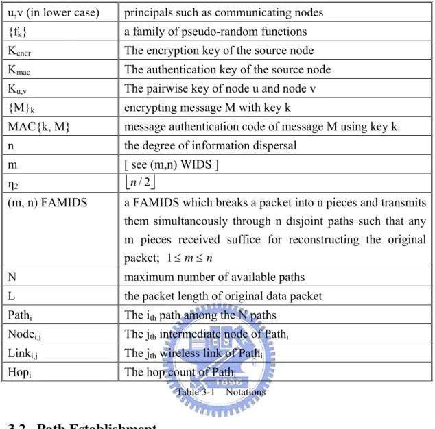
(16) sensor node is compromised, all the confidential information it holds will be known to the attacker. In addition, since the wireless communication is inherent insecure, we assume an adversary can eavesdrop on all traffic, inject packets, or replay packets. However, we assume that the base station will not be compromised. Finally, to secure packet transmission, we assume some existent secure key establishment and management protocols, such as LEAP [18], is incorporated into the system. We assumed that at least the following keys are securely established:. 1) Individual key: Every node shares a unique individual key with the base station. Assume the individual key of node u is Ku, node u can generate the encryption key and authentication key by Ku and a pseudo random function f:. K encr = f Ku (0), K mac = f Ku (1) 2) Pairwise key: Every node shares a unique pairwise key with each of its immediate neighbors. 3) Cluster key: Every node shares a key with all its neighbors. In FAMIDS, we only consider the security of data packet transmission. We assume the security of all keying mechanisms is guaranteed by the key establishment and management protocol, and the security of path establishment and maintenance is assured by the disjoint multipath routing protocol.. Notations. We list below the notations which appear in the explanations of. FAMIDS.. 9.

(17) u,v (in lower case). principals such as communicating nodes. {fk}. a family of pseudo-random functions. Kencr. The encryption key of the source node. Kmac. The authentication key of the source node. Ku,v. The pairwise key of node u and node v. {M}k. encrypting message M with key k. MAC{k, M}. message authentication code of message M using key k.. n. the degree of information dispersal. m. [ see (m,n) WIDS ] ⎣n / 2⎦. η2 (m, n) FAMIDS. a FAMIDS which breaks a packet into n pieces and transmits them simultaneously through n disjoint paths such that any m pieces received suffice for reconstructing the original packet; 1 ≤ m ≤ n. N. maximum number of available paths. L. the packet length of original data packet. Pathi. The ith path among the N paths. Nodei,j. The jth intermediate node of Pathi. Linki,j. The jth wireless link of Pathi. Hopi. The hop count of Pathi Table 3-1. Notations. 3.2. Path Establishment Path establishment consists of three main phases: path discovery phase, path evaluation phase and path maintenance phase. We explain the operations of each phase below.. Path discovery phase. Path discovery phase is initiated by a source node that has. some sensed information for the base station and no valid routing entry in its routing table. The source node adopts disjoint multipath routing protocol to construct multiple paths to the base station. We assume that any disjoint multipath routing protocols for wireless sensor networks can be adopted to acquire these paths. After path discovery 10.

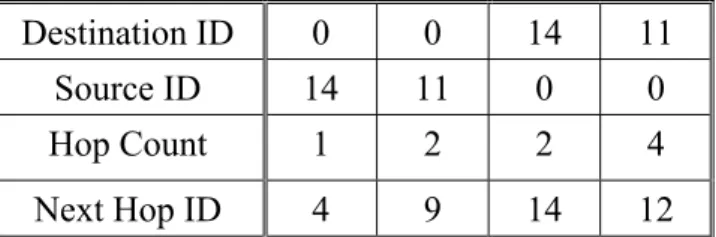
(18) finished, N disjoint paths are established and considered as ideally independent, which means they have no intermediate nodes in common. After. path. discovery. phase finished, all the involved sensor nodes will possess the up-to-date routing information. The intermediate nodes will set up both the forward path (the source node to the base station) and the reverse path (the base station to the source node).. The following figure shows a simplified example of path discovery phase. Figure 3-1(a) shows the topology of the sample network, which consists of one base station and fifteen sensor nodes. Each node has a unique ID and in this example, the base station ID is 0. The dashed lines represent the communication range of the sensor nodes. Node 14 and Node 11 successively initiate path discovery phase to acquire three disjoint paths to the base station. Figure 3-1(b) and Figure 3-1 (c) show the paths constructed by Node 14 and Node 11 after the path discovery phase finished, respectively. The updated routing information is then stored in the routing table of each involved node. Table 3-2 and Table 3-3 show the related entries of routing table of Node 8 (an intermediate node) and Node 11 (a source node), respectively.. Figure 3-1 Path discovery phase. Destination ID. 0. 0. 14. 11. Source ID. 14. 11. 0. 0. Hop Count. 1. 2. 2. 4. Next Hop ID. 4. 9. 14. 12. Table 3-2 Routing table of Node 8 11.

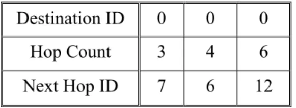
(19) Destination ID. 0. 0. 0. Hop Count. 3. 4. 6. Next Hop ID. 7. 6. 12. Table 3-3 Routing table of Node 11. Path evaluation phase The source node must have the knowledge of successful transmission probability of the paths to perform FAMIDS. It is noted that the established paths have different hop counts and also different successful transmission probability. There are several ways to acquire the successful transmission probability of each path. One viable approach is to utilize the link quality parameter implemented by RF module (e.g. LQI, RSSI) to indicate the successful transmission probability of wireless links. One viable approach is that the base station periodically broadcasts a link quality estimation packet. Each intermediate node receiving the packet appends the bit error rate indicated by the LQI parameter to the packet and retransmits the packet to source nodes through the reverse paths. The source nodes can update the success probability of the paths according to the received packet.. Another mechanism can cooperate with the link quality estimation mechanism to acquire better knowledge of successful transmission probability of each path. The base station that acts as a network coordinator keeps monitoring the network traffic and keeps tracking of the number of successfully transmitted packets of all paths. Compared with the results of the two mechanisms, the base station can possibly detect node compromise.. Path maintenance phase After multiple paths are established, the multipath routing protocol is responsible for maintaining the availability of multiple paths. Many 12.

(20) multipath routing protocols provides mechanisms to detect node failures, such as link-layer ACK, and periodical HELLO message broadcast, etc. If a node failure is detected by its upstream neighbor, the neighbor may send packets to notify the affected source nodes. The notified source nodes may decide whether to re-initiate the path discovery phase according to the remaining number of available paths.. 3.3. Packet Transmission After the path establishment phase is finished, the source node will construct N paths to the base station, and simultaneously obtain the successful transmission probability of the paths. The source node is then able to transmit the data packets using (m, n) FAMIDS. We categorize the operations of packet transmission into three phases, packet generation phase, packet splitting phase and packet transmission phase, and explain separately.. Packet generation phase In order to provide secure communication between the source node and the base station, some security mechanisms are needed before packet splitting. Assume the original information sensed by the source node is M. The source node performs some encryption and authentication operations on M, and the message becomes:. D = {M || MAC (K mac , M || S )} K encr In the modified message D, S represents the sequence number shared secretly between the source node and the base station which indicates the order of the transmitted packets. The maintenance and synchronization of the sequence number of the two ends can be achieved by some existing security mechanism, such as SPINS. Without loss of generality, we assume the length of the modified message to be L bits.. 13.

(21) Packet splitting phase In FAMIDS, a uniform allocation approach is taken, which means all paths used for transmission are assigned with one subpacket, in order to have the advantage of load balance. Based on the successful transmission probability of available multiple paths, the source node decides the optimal (m, n) FAMIDS with the highest communication reliability, where 1 ≤ n ≤ N ,1 ≤ m ≤ n . Compared with the. brute-force approach that examining all the (m, n) pairs taken by other schemes, in FAMIDS the base station only needs to consider the communication reliability of the reduced candidate set of (m, n) pairs. In the analysis section, an efficient algorithm for determining the candidate set of (m, n) pairs is proposed.. After determining the optimal (m, n) pair, the source node splits the modified message D of L bits into n sub-packet Di, 1 ≤ i ≤ n , each of length L/m. In order to solve the sharing problem of the secret matrix A between the source node and the base station, we attach the row Ai of matrix A in front of the sub-packet Di, where 1 ≤ i ≤ n , rather than negotiating the matrix A in advance. Algorithm 3-1 shows the basic packet splitting algorithm, where the Mi, 1 ≤ i ≤ n , computed from the last step are the final sub-packets the source node transmits to the base station. The total computational overhead of the basic algorithm is O(m2).. There are two important observations of FAMIDS in wireless sensor networks. First, the original data packets are of equal size. Second, the maximum number of available paths, i.e. N, is determined before deployment. Benefit from the observations, the base station preloads each sensor node with sufficient pre-computed sets of rows of matrix A with a sufficient large prime p, and each transmission the source node forms the matrix A by the first m elements of randomly choosing n rows 14.

(22) from the pre-computed set. Earlier research has discussed on the appropriate multipath level for wireless sensor networks and indicated that excessive multipath level does not benefit the data transmission because of the maintenance overhead. As a result, the degree of information dispersal, i.e. n, should be relative small in wireless sensor networks; it is efficient to trade storage for computation. With the modified packet splitting algorithm 3-2, the source node only needs to attach the first element ri in front of the sub-packet Di to notify the base station of secret matrix A, and thus saving communication bandwidth. Algortihm 3-1: Basic_Paket_Splitting (D, m, n). 1. Choose a prime p that p> 2 m − 1 2. Randomly choose n different elements ∈ Z p , denoted by r1, r2, …, rn 3. Computes the rows of matrix A. [. ]. ai = 1, r1 , r12 ,L, r1m −1 , 1 ≤ i ≤ n. 4. Splits D into L/m pieces, each piece of length m. (if L is not a multiple of m, pad 0 to the last piece), denoted by S1 , S 2 ,L, S L . m. 5. Computes the sub-packets Di , 1 ≤ i ≤ n by Di = ⎡ai S1 , ai S 2 ,L, ai S L ⎤ ⎢⎣ m⎥ ⎦ 6. Append ai to Di, M i = ai || Di , 1 ≤ i ≤ n . Algorithm 3-2: Modified_Paket_Splitting (D, m, n) 1. Randomly choose n rows from the pre-computed set of matrix A, each row. [. ]. takes the first m elements, i.e. ai = 1, r1 , r12 ,L, r1m −1 , 1 ≤ i ≤ n. 2. Splits D into L/m pieces, each piece of length m. (if L is not a multiple of m, pad 0 to the last piece), denoted by S1 , S 2 ,L, S L . m. 3. Computes the sub-packets Di , 1 ≤ i ≤ n by Di = ⎡ai S1 , ai S 2 ,L, ai S L ⎤ ⎢⎣ m⎥ ⎦ 4. Append ri to Di, M i = ri || Di , 1 ≤ i ≤ n . Packet transmission phase The intermediate nodes all keep a specific sequence 15.

(23) number of its upstream and downstream neighbors to indicate the number of packets that are successfully received or transmitted by them. For example, Su,v represents the number of successful transmitted packets from node u to node v. Like the sequence number S, the value of each sequence number between two neighbors is maintained by SPINS. After packet splitting phase is finished, the source node transmits the sub-packets Mi’s through the multiple disjoint paths to the base station. The following equations show the transmission process of the sub-packets:. {. Source Node Æ Nodei,1: Mi|| S source,nodei ,1. {. Nodei,jÆ Nodei,j+1: Mi || S nodei , j ,nodei , j +1. }. K source ,nodei ,1. }. K node. , 1≤ i ≤ N. , 1 ≤ j ≤ Hopi − 1 i , j , nodei , j +1. The first equation shows the transmission operations of the source node, while the second one represents the transmission operations of the intermediate nodes. Each intermediate node first verifies the received sub-packet by the encrypted sequence number in the rear of the packet. If a valid sub-packet is recognized, the intermediate node replaces the second part of the sub-packet and re-transmits the sub-packet to the downstream neighbor. The whole transmission process continues until the base station, i.e. Nodei , Hopi , receives the sub-packet. If enough sub-packets are correctly received by the base station, the base station can reconstruct the original information based on the secret matrix A and the encryption and authentication keys shared with the source node. Explicit acknowledgment and retransmissions can also be incorporated to enhance the system reliability if needed.. In the following section, we analyze the communication reliability and information security of FAMIDS and some efficient algorithm are proposed to determine the optimal set of (m, n) with highest communication reliability under different network conditions. 16.

(24) 4. Analysis In this section, we analyze the performance of FAMIDS for two aspects: communication reliability and information security. Regarding reliability, we begin with some preliminary knowledge. The communication reliability of FAMIDS, R(m, n) is then derived as an analytical form. In the next sections, we analyze the behavior analytical form under different network conditions and propose separately efficient ways for finding the optimal set of (m, n) with highest communication reliability. In addition, as far as security is concerned, we analyze the security level achieved by FAMIDS for the following concerns: information confidentiality, message integrity and attack resistance. We detail the countermeasures of FAMIDS to resist above-mentioned security problems.. 4.1. Reliability Analysis. In this section, we analyze the optimal communication reliability that FAMIDS achieves under four different network conditions: simple case, ideal case, general case and special case. The following analysis is based on the hardware specification of current generation sensor nodes. In addition, since the multipath level of a general sensor network should be relative small, a maximum multipath level of 10 is discussed in the following analysis. The proof of the theorems and corollaries derived in this section is provided in the appendix.. 4.1.1. Preliminary. We would like to start our reliability analysis with some preliminary knowledge 17.

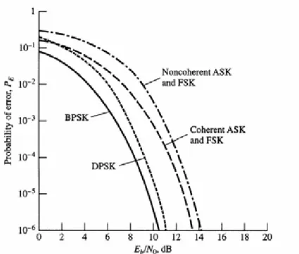
(25) about the characteristics of wireless channel and the influence of packet splitting.. •. Characteristics of wireless channel. Table 4-1 summarizes the hardware specification of the radio frequency modules embedded in the Berkeley MICA series nodes [15]. With different signal modulation techniques, the relationship between signal-to-noise ratio (SNR) and bit error rate (BER) varies, as shown in Figure 4-1. In the equation of BER, Eb is defined as the ratio of energy per bit and N0 represents the spectral noise density. It is easy to find that the increase in SNR will cause a decrease in BER. We can also observe that, under the same sensing environment, binary phase shift keying (BPSK) has better performance.. For a wireless link between two sensor nodes like Figure 4-2(a), the link success probability that a packet of length L bits can successful transmit from one node to the other is Pl = (1 − Pb ) L. (1). In equation (1), Pb represents the BER of the wireless link. Figure 4-2(b) gives us an example to illustrate the relationship between BER and Pl. In this example, we assume a packet of 28 bytes is transmitted through a BPSK channel between two nodes. We can observe from the graph that the link success probability drops drastically to 0.1 when BER approaches to 0.01.. 18.

(26) Senor Node. RF Chip. Signal Modulation Techniques. Bit error rate. MICA. TR1000. Amplitude Shift Keying (ASK). Pb = Q Eb / N 0. MICA2. CC1000. Frequency Shift Keying (FSK). Pb = Q Eb / N 0. MICAZ. CC2420. Binary Phase Shift Keying (BPSK). Pb = Q 2 Eb / N 0. Table 4-1 The Spec. of MICA series sensor nodes. Figure 4-1 Relationship between BER and SNR. Figure 4-2 An example of link success probability. 19. (. ). (. ). (. ).

(27) •. The influence of packet splitting on link success probability. Based on the results derived in the previous section, here we would like to explain the influence of packet splitting on link success probability. The link success probability of transmitting the original packet of length L bits is Pl = (1 − Pb ) L. (2). If we split the original packet into several sub-packets, each of size L/2 bits, the link success probability becomes L 2. Pl = (1 − Pb ) = Pl '. (3). Similarly, if we split the original packet into several sub-packets, each of size L/m bits, m ≥ 1 , the link success probability afterwards turns into Pl ' = (1 − Pb ) L / m = m Pl. (4). Because of 0<Pl<1 and m ≥ 1, the link success probability after packet transmitting is greater or equal to the original link success probability. Figure 4-3 shows the link success probability with or without packet splitting approach. Each line in the graph represents the link success probability of different packet size. Two conclusions we can draw from Figure 4-3. First, the link success probability is greatly improved when the original Pl is small. In other words, if the BER of the wireless link is bigger, we can achieve larger link success probability gain resulted from packet splitting. Second, the probability gain from packet length L to L/2 is the biggest. The two conclusions will dominate the results of our reliability analysis.. 20.

(28) Figure 4-3 The effect of packet splitting. •. The path success probability. To facilitate the following analysis, we would like to explain the formation of path success probability first. For a path of H hops, there are H-1 intermediate nodes and H links between nodes. Figure 4-4 plots a path of 4 hops from a source node to the base station. The path success probability is composed of the success probabilities of the links and the intermediate nodes. It is noted that the path success probability is influenced by the packet length. Assume Pl,i and Pn,i represent the success probability of the ith link and the ith intermediate node when transmitting a L-bit packet respectively, the path success probability is H. H −1. H. H −1. i =1. i =1. i =1. i =1. Ps = ∏ Pl ,i × ∏ Pn ,i = ∏ (1 − Pb ,i ) L × ∏ Pn ,i = PL × PN. (5). For simplicity, we use PL and PN to represent the cumulative link success probability and cumulative node success probability. We will use the definition in the following analysis interchangeably. When (m, n) FAMIDS is applied, the original L-bit packet is fragmented into n sub-packets of length L/m bits. As a result, the path 21.

(29) success probability when transmitting a sub-packet becomes H. H −1. H. i =1. i =1. H −1. L m. Ps = ∏ P × ∏ Pn ,i = ∏ (1 − Pb ,i ) × ∏ Pn ,i = m PL × PN '. ' l ,i. i =1. (6). i =1. Compared with the two equations, we have found that the success probability of intermediate nodes is independent of packet size. The reason is that node success probability is influenced by energy depletion of sensor nodes, while the BER of sensing environment dominates the link success probability. When performing analysis, we usually ignore the problem of energy depletion and assume the involved nodes have efficient energy for packet transmission. As a result, we can simplify the equations as: H. H. i =1. i =1. Ps = ∏ Pl ,i = ∏ (1 − Pb ,i ) L H. H. L m. Ps = ∏ P = ∏ (1 − Pb ,i ) = m Ps '. i =1. ' l ,i. (7) (8). i =1. In the following section, we will derive the analytical form of the communication reliability of (m, n) FAMIDS, i.e. R(m, n), based on the above two equations.. Figure 4-4 A multi-hop path. 22.

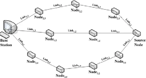
(30) 4.1.2. The Communication Reliability R(m, n). Figure 4-5 The wireless sensor network model. In our network model, we assume that N disjoint paths are available for data packet transmission from a source node to the base station. Figure 4-5 plots an example of N=3, where the Nodei,j and Linki,j means the jth intermediate node and the jth link of path i, respectively. If the source node decides to transmit the original data packet of length L bits by (m, n) FAMIDS, the packet is fragmented into n sub-packets of length L/m, where 1 ≤ n ≤ N , 1 ≤ m ≤ n . It is noted that a decision to use n paths means that these paths will be the first n ones with the highest success probability, in order to achieves the optimal reliability. The success probabilities of the n paths when transmitting the original packet of length L bits are organized in the probability vector Ps = [Ps,i], 1 ≤ i ≤ n . For easy to explain, we order the paths from the best one to the worst one, i.e. Ps,i ≥ Ps,i+1. When (m, n) FAMIDS is applied, the size of sub-packet reduces to L/m and the probability vector turns into Ps' = [ m Ps ,i ] , 1 ≤ i ≤ n . Given the fact that uniform allocation is adopted, we define a state vector s=. [si], 1 ≤ i ≤ n to indicate the the number of sub-packets that actually reach the base 23.

(31) station through the n paths. There are only two possible values for si, i.e. 0 and 1. If si=0, the number of successful transmitted sub-packets through path i is 0. On the other hand, si=1 indicates the assigned sub-packet of path i actually reaches the base station. The associated probabilities are: Pr{si = 1}= m Ps ,i. (10). Pr{si = 0}=1- m Ps ,i. (11). The communication reliability of (m, n) FAMIDS, which denotes as R(m, n), is that the base station can reconstruct the original data packet by the successfully received sub-packets. Since the base station can rebuild the original data packet only if more than m correctly received sub-packets, we can define R(m, n) as ⎧n ⎫ R(m, n) = Pr ⎨∑ si ≥ m⎬ ⎩ i =1 ⎭. •. (12). Formula of R(m, n). It is easy to understand that there are total 2n possible states of s. The probability that the n paths are in state s can be calculated as n. p(s) = ∏ i =1. (. m. Ps ,i. ) × (1 − si. m. Ps ,i. ). 1− si. (13). We classified all possible states of s into n+1 classes according to the number of successfully transmitted paths, which denotes as Sk. ⎧ n ⎫ S k = ⎨s : ∑ si = k ⎬ , 0 ≤ k ≤ n ⎩ i =1 ⎭. (14). The size of class Sk is C kn . Given the classification of all possible states, we can rewrite the communication reliability R(m, n) as R(m, n) =. n. ∑ ∑ p( s). k = m s∈S k. 24. (15).

(32) Based on the formula of R(m, n), we analyze the behavior of R(m, n) under four different cases of network in the following sections. For each network condition, we derive an efficient way or algorithm for determining the optimal (m, n) with highest communication reliability.. 4.1.3. The Simple Model. First of all, the simple model to be analyzed is illustrated as Figure 4-6. N disjoint paths are constructed from source node to base station for packet transmission. In the simple model, we assume that the influence of packet splitting on path success probability is so trivial that we can ignore the probability gain. That is, '. Ps = [ m Ps ,i ] ≅ [ Ps ,i ] = Ps. (16). This is the case that the BER of the sensing environment is relative small and thus the probability gain of link success probability achieved by FAMIDS can be ignored. In other word, the path success probability is independent of packet length.. Figure 4-6 The simple model. 25.

(33) Assume that the source node uses (m, n) FAMIDS for packet transmission, 1 ≤ n ≤ N ,1 ≤ m ≤ n . Based on the definition of the simple model, the probability that n paths are in state s turns into p(s) = ∏ (Ps ,i ) i × (1 − Ps ,i ) n. 1− si. s. (17). i =1. As a result, the communication reliability of the simple model can be derived as R(m, n) = ∑ ∑∏ (Ps ,i ) i × (1 − Ps ,i ) n. n. s. 1− si. (18). k = m s∈S k i =1. Theorem 4-1 to Theorem 4-3 discuss the relationship between R(m, n)’s and help us find the optimal set of (m, n) with the optimal communication reliability.. Theorem 4-1: R(m, m)>R(m+1, m+1), for 1 ≤ m ≤ N − 1. Theorem 4-1 concludes that among all FAMIDS that information expansion ratio is 1, the communication reliability of (1, 1) FAMIDS is maximum.. Theorem 4-2: R(m, n)<R(m, n+1), for 1 ≤ n ≤ N − 1 , 1 ≤ m ≤ n. For. example, R(2,3) − R(2,2) = Ps ,3 × [ Ps ,1 × (1 − Ps , 2 ) + (1 − Ps ,1 ) × Ps , 2 ] ,. and. R (3,4) − R (3,3) = Ps , 4 × [ Ps ,1 × Ps , 2 × (1 − Ps ,3 ) + Ps ,1 × (1 − Ps , 2 ) × Ps ,3 + (1 − Ps ,1 ) × Ps , 2 × Ps ,3 ] .We observe that every term in the examples is positive, so the difference of communication reliability is also positive. Theorem 4-2 suggests that the communication reliability can be improved if more subpackets are sent and the same number of subpackets is needed for rebuild the original packet.. Theorem 4-3: R(m, n)>R(m+1, n), for 1 ≤ m ≤ n − 1. 26.

(34) Theorem 4-3 tells us that if the same number of paths is used, the communication reliability increases as fewer subpackets are needed for rebuilding the original information.. Although the previous three theorems do not discuss all the relationship between all possible pairs of (m, n), the results is sufficient for us to find the optimal (m, n) FAMIDS in the simple network model. For example, if there are total 5 disjoint paths available for the source node, 15 combinations of (m, n) MIDS can be selected. We summarize the results derived from the three theorems and thus we can get the optimal solution: 1) 2) 3) 4) 5) 6) 7) 8) 9). R(1, 1)>R(2, 2)>R(3, 3)> R(4, 4)> R(5, 5) R(1,5)>R(1,4)>R(1,3)>R(1,2)>R(1,1) R(2,5)>R(2,4)>R(2,3)>R(2,2) R(3,5)>R(3,4)>R(3,3) R(4,5)>R(4,4) R(1,5)>R(2,5)>R(3,5)>R(4,5)>R(5,5) R(1,4)>R(2,4)>R(3,4)>R(4,4) R(1,3)>R(2,3)>R(3,3) R(1,2)>R(2,2). From the results, we can conclude that (1,5) IDS is the optimal solution when there are totally 5 paths available. Corollary 1 is thus established.. Corollary 1: If the path success probability is independent of packet size , (1, N). FAMIDS is always the optimal solution.. In this simple network case, since the link failure rate is negligible, the probability gain achieved by FAMIDS is limited. In other words, packet splitting does not benefit 27.

(35) the communication reliability. As a result, splitting the original data packet with the maximum information expansion ratio, i.e. (1, N) FAMIDS, always achieves the optimal communication reliability. Algorithm 4-1 summarizes the analysis results of this section and shows how to find the optimal m value under simple network model. In the next section, we consider an idealized network case that the influence of packet splitting is taken into consideration. Algorithm 4-1: Finding Optimal m for (m, N) FAMIDS under Simple Model Input: N: number of total available paths. Output: m: the optimal value of m, such that (m, N) FAMIDS achieves the optimal communication reliability. 1. The optimal m value is 1. 2. If the optimal m cannot satisfy the information expansion ratio requirement, then choose m=2, m=3, …, m=N respectively, until the information expansion ratio is satisfied. 3. Output m. 4.1.4. The Ideal Model. In the section, we analyze the behavior of R(m, n) under an idealized network. The network topology is the same as the simple model, except that each path has the same success probability where the problem of node failure is still ignored. That is, Ps,i=Ps, ∀1 ≤ i ≤ n. (19). As a result, each state s in the same class Sk has the same probability, which can be derived as p(s) =. ( P ) × (1 − m. k. s. m. Ps. ). n−k. if s ∈ Sk. (20). Therefore, R(m, n) can be expressed as R(m, n) =. n. ∑ ∑ p( s) =. k = m s∈S k. ∑C ( n. k =m. n m k. Ps. ) × (1 − k. m. Ps. ). n−k. (21). The behavior of the communication reliability R(m, n) under ideal case is. 28.

(36) equivalent to the analysis results provided in [10]. We summarize the behavior of R(m, n) as follows:. 1) When using total available paths, one gets the highest communication reliability.. 2) If N paths are available for packet transmission, the optimal (m, n) FAMIDS is in the candidate set {(i, N) FAMIDS | 1 ≤ i ≤ η 2 }. Figure 4-7 gives an example to illustrate the relationships between R(1,N), R(2, N), …, and R(η2,N). We can observe that a particular FAMIDS does not always give better reliability than another. According to the value of Ps and the critical probability of (i, N) FAMIDS and (i+1, N) FAMIDS, one can determine the (m, N) FAMIDS with highest communication reliability. Table 4-2 summarizes the intersections of R(m, n) for m=4..10. Based on Table 4-2, Algorithm 4-2 can determine the optimal (m, N) FAMIDS with optimal communication reliability under ideal network model.. 3) If the upper bound on information expansion ratio is given, i.e. u, the candidate FAMIDS set Cu,N is reduced to. {(i, i * u )FAMIDS | 1 ≤ i ≤ η u } U {(η u +. j , N )FAMIDS | 1 ≤ j ≤ N − η u. and η u + j ≤ η 2 } when u ≥ 2 ,. (22). or. {(i, i * u )FAMIDS | 1 ≤ i ≤ η u } U (η u + 1, N )FAMIDS when. u ≤ 2.. (23). The ηu and η2 in (22) and (23) means the value of ⎣N / u ⎦ and ⎣N / 2⎦ , respectively. The source node only needs to check the communication reliability of the candidate set to determine the optimal set.. 29.

(37) Figure 4-7 Relationships between R(1,N) to R(4,N). j. Ps*[(1,j),(2,j)]. 4. 0.271837. 5. 0.579696. 6. 0.768788. 0.022815. 7. 0.874048. 0.132044. 8. 0.931467. 0.294322. 0.001058. 9. 0.962716. 0.457744. 0.016607. 10. 0.979738. 0.597068. 0.065319. Ps*[(2,j),(3,j)]. Table 4-2. Ps*[(3,j),(4,j)]. Ps*[(4,j),(5,j)]. 0.000032471. The intersections: Ps*[(i,j),(i+1,j)]. Algorithm 4-2: Finding Optimal m for (m, N) FAMIDS under Ideal Model Input: N: number of total available paths Input: Ps: the path success probability. Output: m: the optimal value of m, such that (m, N) FAMIDS achieves the optimal communication reliability. 1. Look up Table 4-2 to determine the region that Ps belongs to. 2. Search the optimal m value as follows. •. If Ps* [(1, N ), (2, N )] < Ps < 1 , then the optimal value of m is 1.. •. If Ps* [(i + 1, N ), (i + 2, N )] < Ps < Ps* [(i, N ), (i + 1, N )] , then the optimal value of m is i+1.. •. If 0 < Ps < Ps* [(η 2 − 1, N ), (η 2 , N )] , then the optimal value of m is η 2 .. 3. If the optimal m cannot satisfy the information expansion ratio requirement, then choose m=m+1, m=m+2 …, m=N respectively, until the information expansion ratio is satisfied. 4. Output m. 30.

(38) In the following section, a more general network model will be analyzed where the restriction on the path success probability under ideal network model is cancelled.. 4.1.5. The General Model. Based on the results of the ideal model, we extend our analysis to a more realistic case, which multiple paths have different success probability. Still, a uniform sub-packet allocation is assumed and the problem of node failures is ignored. To facilitate our following analysis, we begin with some more definitions. We define a function Fk(n) to represent the sum of probabilities that all states s that belongs to Sk when n paths are being used for packet transmission Fk(n)=. ∑ p( s) ,. 0≤k ≤n. (24). s∈S k. In addition, we define the sums of function F from class k to class n n. n. i =k. j =k. Fk’(n)= ∑ Fi (n) = ∑ m Ps , j ⋅ Fk −1 ( j − 1). (25). The equivalence of the two sums of equation (19) is proved in [13]. As a result, the expression for R(m, n) found in (15) can be rewritten as R(m, n) = Fm’(n). (26). The following theorem can explain the relationships between R(m, n) with a fixed value of m for 1 ≤ n ≤ N .. Theorem 4-4: R(m, n) < R(m, n+1), for 1 ≤ m ≤ n. Based on Theorem 4-4, we can conclude that one can achieve the highest communication reliability when all available paths are used. If total N paths are. 31.

(39) available for transmission, the candidate FAMIDS set can be reduced to {(m, N) FAMIDS | 1 ≤ m ≤ N }. This conclusion is the same as the ideal case. However, because of the variety of path success probabilities, the influence of packet splitting for each path is different. As a result, even if the number of available paths and the average success probability of the paths are the same, the optimal set of (m, N) with highest communication reliability may be different. For example, assumed that 6 disjoint paths are available for transmission and average success probability is 0.75. If the probability vector Ps is [0.8, 0.8, 0.75, 0.75, 0.75, 0.65], (2, 6) FAMIDS achieves the highest communication reliability. On the other hand, (1, 6) FAMIDS becomes the optimal solution when Ps is [0.85, 0.8, 0.8, 0.7, 0.7, 0.65]. The variety of the optimal solutions results from the variety of path success probabilities.. However, resorting to simulation, we have observed that there are still some combinations between the results of the ideal model and the general model. First, the candidate FAMIDS set of both network models ranges from (1, N) FAMIDS to (η2, N) FAMIDS, where η2= ⎣N / 2⎦ . In other words, (η2+1, N) FAMIDS to (N, N) FAMIDS can not be the optimal solution under both ideal model and general model. Second, according to the average success probability of paths Ps and the critical probabilities of (m, n) FAMIDS found in ideal case, one can determine a more exact candidate FAMIDS set, which denotes as CN: 1) If Ps* [(1, N ), (2, N )] < Ps < 1 , CN={(m, N) FAMIDS | m=1 }. 2) If Ps* [(i + 1, N ), (i + 2, N )] < Ps < Ps* [(i, N ), (i + 1, N )] , CN={(m, N) FAMIDS | m=1..i+1}. 3) If 0 < Ps < Ps* [(η 2 − 1, N ), (η 2 , N )] , CN={(m, N) FAMIDS | m=1..η2}. 32.

(40) Compared with the brute-force approach taken by other schemes that examining all the possible pairs of (m, n), where 1 ≤ n ≤ N ,1 ≤ m ≤ n , in FAMIDS the source nodes only need to check the (m, n) pairs in the reduced candidate set CN. Algorithm 4-3 shows how to find the optimal value of m. The algorithm reduces the complexity of finding the candidate set of (m, n) from O(N2) to O(N). Algorithm 4-3: Finding Optimal m for (m, N) FAMIDS under General Model Input N: the number of available paths. Input Ps : the probability vector Output: m: the optimal value of m, such that (m, N) FAMIDS achieves the optimal communication reliability. 1. Calculate the average success probability Ps =. N. ∑P i =1. s ,i. N.. 2. Look up Table 4-2 to determine the region that Ps belongs to. 3. Determine the reduced candidate FAMIDS set CN as follows. •. If. Ps* [(1, N ), (2, N )] < Ps < 1. •. If. Ps* [(i + 1, N ), (i + 2, N )] < Ps < Ps* [(i, N ), (i + 1, N )]. , CN={(m, N) FAMIDS | m=1 }. , CN={(m, N) FAMIDS. | m=1..i+1}. •. * ( )( ) If 0 < Ps < Ps [ η 2 − 1, N , η 2 , N ] , CN={(m, N) FAMIDS | m=1..η2}.. 4. Calculate the communication reliability of (m, N) FAMIDS in CN. Assume that (m’, N) FAMIDS achieves the optimal reliability. 5. If the optimal m=m’ cannot satisfy the information expansion ratio requirement, then choose m=m’+1, m=m’+2, …, m=N respectively, until the information expansion ratio is satisfied. 6. Output m.. 33.

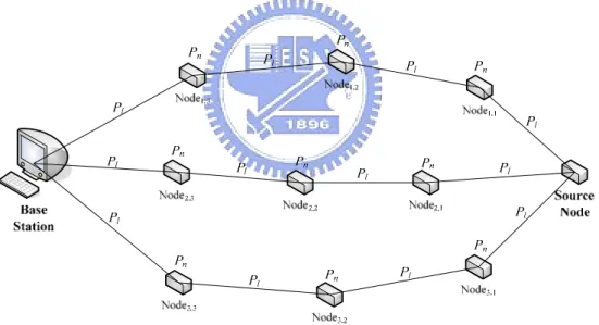
(41) 4.1.6. The Special Model. The previous analysis of the general network model is based on the assumption that node failures can be ignored. However, in a realistic network, the situation is usually more complicated with the existence of node compromise. In order to realize the effect of node failures, we illustrate a special example of network environment to explain the influence of node failure over R(m, n). Figure 4-8 shows the special network model, where N disjoint paths with identical number of hops and success probability are considered. All wireless links and intermediate nodes have the same success probability respectively, which are denoted as Pl and Pn. That is, the influence ratio of the two factors is fixed under special network model.. Figure 4-8 The special network case. Based on the assumptions of the network environment, the original path success probability is the same as equation (5). When (m, n) FAMIDS is applied, the path success probability of transmitting a sub-packet of L/m bits can be expressed as equation (6). Using (m, n) FAMIDS, the base station can reconstruct the original information if more than m sub-packets are correctly received. As a result, the 34.

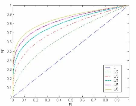
(42) communication reliability R(m, n) can be modified as equation (27): R (m , n ) =. n. ∑C i=m. n i. ⋅ ⎛⎜ ⎝. ( P) m. H. l. i. ⋅ PnH −1 ⎞⎟ ⋅ ⎛⎜ 1 − ⎠ ⎝. ( P) m. ⋅ PnH −1 ⎞⎟ ⎠. H. l. n −i. (27). On account of the definition of cumulative node and link success probability, equation (27) can be rewritten as R (m , n ) =. ∑C ⋅( n. i=m. n i. m. PL ⋅ PN. ) ⋅ (1 − i. m. PL ⋅ PN. ). n −i. (28). Figure 4-9 illustrates an example of the relationship between the original Ps and the communication reliability after (m, 6) FAMIDS is applied. In this example, the number of hops is 3 and the node success probability Pn is 0.9. As shown in Figure 4-9, we can observe that the communication reliability is greatly improved when the original path success probability is relative small because of the increase in the link success probability. In order to determine the optimal (m, n) set with the highest communication reliability under different Ps, some fundamental theorems regarding the relationship between R(m, n)’s are derived.. Figure 4-9 Relationship between Ps and (m,6) MIDS. 35.

(43) •. Fundamental Theorems. Here are some fundamental theorems that the results help us to determine the optimal value of (m, n) set with highest communication reliability.. Theorem 4-5: R(m, n) is strictly increasing for 0 < Ps < 1.. Theorem 4-5 implies that the communication reliability achieved by a specific (m, n) FAMIDS is proportional to Ps. When the successful transmission probability of each path increases, the communication reliability is also improved.. Theorem 4-6: if 0 < Ps < 1, then R(m, n)< R(m, n+1).. Theorem 4-6 suggests the communication reliability can be improved if more pieces of sub-packets are sent and the same number of sub-packets is needed to reconstruct the original data packet. Figure 4-10 shows the distribution of the reliability curves of (1, n) MIDS, where 1 ≤ n ≤ 6 , and each path has 3 hops with Pn=0.9. The results implied in Figure 4-10 are consistent with Theorem 4-6.. 36.

(44) Figure 4-10 Relationship between the Ps and (1,n) MIDS. Theorem 4-7: R(m, n) > R(m+1, n) when PsÆ1-. From Theorem 4-7, we can observe that the fewer the number of sub-packets needed to reconstruct the original data packet, the higher the communication reliability when the message dispersal degree n is fixed and Ps is approaching to 1. The only likelihood that Ps is approaching to 1 is both Pl and Pn are approaching to 1. As a result, we can infer Corollary 2 from Theorem 4-7.. Corollary 2: R(1, n) is the optimal of R(i, n) when PsÆ1-, for 1 ≤ i ≤ n .. Under the condition that Ps is approaching to 1, it means that both the node and link failure rate are relative small and thus the effect of packet splitting is so trivial that can be neglected. As a consequence, the maximum information expansion ratio achieves the optimal reliability under such network condition. The result is also consistent with the simple model. Compared with the case when PsÆ1-, the case when PsÆ0+ is more complicated. Theorem 4-8 & Theorem 4-9 give the explanation of such case. 37.

(45) Theorem 4-8: R(η,n) is the optimal of R(i, n) when Pl Æ 0+, for 1 ≤ i ≤ n , ⎡ P ⋅ n − 1⎤ where η = ⎢ N ⎥ ⎢ PN + 1 ⎥. Theηvalue derived by Theorem 4-8 is a critical number of (m, n) FAMIDS. When link success probability is approaching to zero, i.e. SNR is extremely small, the optimal (m, n) set is mainly determined by node success probability. From Theorem 4-8, we can guarantee the correctness of Corollary 3 & Corollary 4.. Corollary 3: R(1, n) is the optimal of R(i, n) when PlÆ0+ and PnÆ0+, for 1≤ i ≤ n.. Corollary 3 conforms to our intuition that the source node should maximize the information expansion ratio when the network is in an exceptionally poor condition. This case happens when the sensor network is deployed in an extremely noisy environment and full of compromised or out-of-battery nodes.. Corollary 4: R(η 2 ,n) is the optimal of R(i, n) when PlÆ0+ and PnÆ1-, for 1 ≤ i ≤ n , where η 2 = ⎣n 2⎦ .. The result of Corollary 4 is similar with the analysis in Tsai’s paper [10] where the sender and receiver share n parallel wireless communication channels with no intermediate nodes. Because of the high node success probability, the communication reliability is mainly constrained by the unreliable links.. 38.

(46) Figure 4-11 shows the relationship between PN and the optimal (m, n) FAMIDS when PlÆ0+ based on Theorem 4-8, for n = 1~10. It is noted that the only optimal solution is (1, n) when number of paths n ≤ 3 . With the decrease in PN, the effect of packet splitting also decreases.. Figure 4-11 Relationship between optimal R(m, n) and PN. Theorem 4-9: R(1, n) is the optimal of R(i, n) when Pn Æ 0+, for 1 ≤ i ≤ n .. From Theorem 4-9, we can conclude that in the circumstance of numerous invalid intermediate nodes, the source node should split the original data packet with maximum information expansion ratio. The result of Theorem 4-9 coincides with the result of Theorem 4-8. 39.

(47) Theorem 4-10: If m ≥ η , then R(m, n) > R(m+1, n).. We can conclude from Theorem 4-10 that the curves of R( η ,n), R( η +1,n),…,R(n,n) do not have intersections. R(η,n) would be the optimal solution if m ≥ η . The next theorem discusses the relationship between R(m, n) if m ≤ η .. Theorem 4-11: If 2 ≤ m ≤ η , then there exists exactly one critical probability. Ps*. ⎧ R (m, n) > R(m − 1, n) when 0 < Ps < Ps* ⎪ such that ⎨ R(m, n) = R(m − 1, n) when Ps = Ps* , where * ⎪ R(m, n) < R (m − 1, n) when P < P < 1 s s ⎩ ⎡ P ⋅ n − 1⎤. η=⎢ N ⎥ ⎢ PN + 1 ⎥. As we can see in Theorem 4-11, in the interval m ≤ η , a particular FAMIDS does not always achieve better communication reliability than another. A FAMIDS can give better reliability in a range of Ps, but worse reliability in the other range. Besides, it is noted that the value ofηdepends on the cumulative node success probability of each path, PN. With the decrease in PN, the value of η also reduces, i.e. fewer pairs of FAMIDS have intersections.. Figure 4-12 shows the relationship between the R(m, n) under different PN, for n = 8, m = 1 ~ 4. In this example, each path has three hops as Figure 4-12. Figure 4-12(a) shows the curves of R(m, n) when Pn=0.9, i.e. η= 4. As we can see, the curves of R(1,8) ~ R(4, 8) have intersections. On the other hand, Figure 4-12(b) represents the curves of R(m, n) when Pn=0.75, i.e.η= 3, such that only R(1,8) ~ R(3, 40.

(48) 8) have intersections. When Pn decreases to 0.65, i.e. η= 2, only the first two curves, R(1,8) and R(2,8), have intersections, as shown in Figure 4-12(c). Finally, we can obviously see that the curves of R(m, n) do not have intersections if η= 1, as shown in Figure 4-12(d).. Figure 4-12. Theorem 4-12: For fixed. R(m, n) under different Pn. n ≥ 6 & PN >. 2 , if n −1. 2 ≤ m ≤ η , then. ⎡ P ⋅ n − 1⎤ Ps* [(m − 1, n ), (m, n )] > Ps* [(m, n ), (m + 1, n)] , where η = ⎢ N ⎥ ⎢ PN + 1 ⎥. Theorem 4-12 proves that the intersections of Ps* [(m + i − 1, n ), (m + i, n )] have increasing order as i increases for fixed n. The following Figure 4-13 shows the relationship between Ps* [i, n] ≡ Ps* [(i, n ), (i + 1, n )] and PN for n = 4 ~ 9. For example, if PN is equal to 0.9 and the number of available paths is 9, the following conclusion 41.

(49) can be drawn: 1) R(1,9) > R(2,9) if Ps> Ps*[1,9] = 0.68 2) R(2,9) > R(3,9) if Ps> Ps*[2,9]= 0.2 3) R(3,9) > R(4,9) if Ps> Ps*[3,9]= 0.0028. We provide the approximation function of each critical probability for different number of available paths in the appendix I to K. The approximation functions can assist the source node with the determination of the optimal (m, n) FAMIDS with highest communication reliability.. Figure 4-13 Relationship between Ps* and PN. 42.

(50) •. Optimal solution discussion. Based on the fundamental theorems derived in this section, we can determine the optimal set of (m, n) FAMIDS with highest communication reliability under special network condition. First of all, according to Theorem 4-6, we can infer that one achieves the maximum communication reliability when total available paths are used for packet transmission. This conclusion holds for each kind of network. Second, about the relationship between all (m, N) FAMIDS, we have found that any particular FAMIDS does not always achieves better reliability than another. According to the knowledge on Ps and PN, one can determine the optimal value of m. Algorithm 4-4 finds the optimal value of m under special network model that achieves the optimal reliability.. Algorithm 4-4: Finding Optimal m for (m, N) FAMIDS under Special Model Input N: the number of available paths Input Ps: the path success probability Input PN: the cumulative node success probability Output: m: the optimal value of m, such that (m, N) FAMIDS achieves the optimal communication reliability. ⎡ P ⋅ N − 1⎤ 1. Calculate the critical number η = ⎢ N ⎥. ⎢ PN + 1 ⎥. 2. Determine the critical probabilities Ps*[(m, N), (m+1, N)] for m=1..η-1 by PN and the approximation functions. 3. Search the optimal m as follows. •. If Ps* [(1, N ), (2, N )] < Ps < 1 , then the optimal value of m is 1.. •. If Ps* [(i + 1, N ), (i + 2, N )] < Ps < Ps* [(i, N ), (i + 1, N )] , then the optimal value of m is i+1.. •. If 0 < Ps < Ps* [(η − 1, N ), (η , N )], then the optimal value of m is η .. 4. If the optimal m cannot satisfy the information expansion ratio requirement, then 43.

(51) choose m=m+1, m=m+2, …, m=N respectively, until the information expansion ratio is satisfied. 5. Output m.. 4.2. Security Analysis In this section, we analyze the security level achieved by FAMIDS. We assume that attacks on sensor network routing in the literature have been tackled by the multipath routing protocols. In our analysis, we put our emphasis on attacks regarding information security. We describe our analysis of FAMIDS as these security concerns: information confidentiality, message integrity, and attack resistance.. 4.2.1. Information Confidentiality. The idea of FAMIDS is originated from the concept of information dispersal scheme that the original information is ruffled and evenly distributed into several sub-packets. Since we incorporate the encryption and authentication procedures into the packet generation phase, an adversary still can not obtain the original information even if enough sub-packets are collected.. 4.2.2. Message Integrity. Message authentication code is utilized to ensure the integrity of sub-packets. By comparing the message authentication code decoded from sub-packets and calculated from the information bits on the fly, the base station can easily identify the integrity of the received packets.. 44.

(52) 4.2.3. Attack Resistance. Traditional packet splitting schemes are susceptible to several attacks, in order to thwart the operation of rebuilding the original information at the base station. We detail our countermeasures to such attacks as follows.. •. Pollution attack. In this attack, an adversary injects forged sub-packets or modifies the context of sub-packets. Traditional packet splitting schemes provide no mechanism for receivers to examine the validity of received sub-packets, and thus receivers fail to reconstruct the original information. In FAMIDS, the source node encrypts the original information and authentication code with the secret key shared with the base station, therefore forged sub-packets can be detected by the base station in advance of information reconstruction.. •. Replay attack. An attacker buffers the correctly received sub-packets from the upstream neighbors, and retransmits the sub-packets afterwards. The sub-packets have not been modified by the attacker and therefore are deemed to be valid from the confidentiality and integrity examination. As a consequence, the receiver will be disturbed by the obsolete sub-packets and reconstruct inconsistent information with the original one generated by the source node. In FAMIDS, we avoid this kind of attack by the sequence number stored in both communicating end. The base station can verify the freshness of a sub-packet by the decoded sequence number. Besides, intermediate 45.

(53) nodes can also confirm the incoming sub-packets by the sequence number shared with upstream neighbors.. 46.

(54) 5. Conclusion In this paper, we propose an enhanced information delivery scheme, FAMIDS, suitable for general applications of resource-restricted wireless sensor networks. Since FAMIDS adopts the concept of packet splitting schemes, and incorporate lightweight security mechanisms, it simultaneously gains the advantages of fault tolerance and information security. We also propose detailed analysis of the communication reliability achieved by FAMIDS. The communication reliability is first derived as an analytical form R(m, n) and is analyzed under four different network models: the simple model, the ideal model, the general model and the special model. For each network model, we derive fundamental theorems to help us understand the behavior of R(m, n) and propose an algorithm separately to determine the optimal (m, n) set with highest communication reliability. From the analysis results of each network model, we can draw some important conclusions:. 1). For any kind of network, one achieves the maximum communication reliability only when total available paths are used for packet transmission.. 2). Transmitting the original packet with the maximum information expansion ratio can not always achieve the best reliability. The reason is that packet splitting causes a drastic gain of link success probability when the BER of the sensing circumstance is relative high. The communication reliability is greatly benefited from packet splitting under such condition.. 3). The optimal solution with the highest communication reliability for total N paths can only be (m, N) FAMIDS, 1 ≤ m ≤ η 2 , where η 2 = ⎣n 2⎦ . Under the circumstance of low link failure rate or high node failure rate, the advantages achieved by packet splitting are then diminished, and thus the candidate set can 47.

(55) be further reduced.. However, there is still no efficient way in the literature to estimate the node failure rate accurately, especially when the adversaries exist. Besides, the base station can make use of the incorrectly received sub-packets to detect the situation of node compromise, and provide a more secure network environment. We leave these challenges as our future work. In addition, although packet splitting mechanism achieves the advantage of fault tolerance, it increases the probability of network congestion simultaneously. Many schemes in the literature consider the problem of network congestion in various networks [4],[5],[16],[17]. We can further combine FAMIDS with some congestion control scheme to achieve better utilization of network bandwidth.. 48.

(56) Appendix A. Proof of Theorem 4.1. R (m, m) − R(m + 1, m + 1) = Ps ,1 × Ps , 2 × L × Ps ,m × (1 − Ps ,( m +1) ) > 0 ∴ R (m, m) > R(m + 1, m + 1) for 1 ≤ m ≤ N − 1. B. Proof of Theorem 4.2. R(m ,n+1)-R(m ,n)=Ps(n+1)×Pr{any m-1 paths success among P1~Pn}>0 ∴ R(m, n) < R(m, n + 1) for 1 ≤ n ≤ N − 1 , 1 ≤ m ≤ n. C. Proof of Theorem 4.3. By the definition of R(m,n), R(m, n)-R(m+1, n)= Pr {m paths success}>0 Î R(m,n)>R(m+1,n). D. Proof of Theorem 4.4. ∵ R(m, n) =. n. ∑. j =m. R(m, n+1)=. n +1. ∑. j =m. m. m. Ps , j ⋅ Fm −1 ( j − 1). Ps , j ⋅ Fm −1 ( j − 1). ∴ R(m, n+1)-R(m, n)=. m. Ps ,n +1 ⋅ Fm −1 (n ) >0. Æ R(m, n+1) > R(m, n). 49.

(57) E. Proof of Theorem 4.5. The first derivative of R(m, n) on Ps is R ' (m, n) = C mn ⋅ m ⋅ Pl. (1− m ) m. ⋅ ( Pl. (1− m ) m. Ps ) m −1 (1 − Pl. (1− m ) m. Ps ) n − m > 0, for 0 < PS < 1. ∴ R(m, n) is strictly increasing for 0 < PS < 1 .. F. Proof of Theorem 4.7. Let γ ( Ps ) ≡ R (m, n) − R (m + 1, n). 1 ⎛ γ ( Ps ) = C ⋅ ⎜⎜1 − Pl m +1 ⋅ Pn ⎝ n 0. ⎛ m1+1 + C ⋅ ⎜⎜ Pl ⋅ Pn ⎝ n m. ⎛ m1 n C1 ⋅ ⎜⎜ Pl ⋅ Pn ⎝. n. ⎞ ⎛ 1 ⎟ + C1n ⋅ ⎜ Pl m +1 ⋅ Pn ⎟ ⎜ ⎠ ⎝. m. 1 ⎞ ⎛ ⎟ ⋅ ⎜1 − Pl m+1 ⋅ Pn ⎟ ⎜ ⎠ ⎝. 1 ⎞ ⎛ m ⎟ ⋅ ⎜1 − Pl ⋅ Pn ⎟ ⎜ ⎠ ⎝. ⎞ ⎟ ⎟ ⎠. n −1. ⎞ ⎟ ⎟ ⎠. n−m. 1 ⎞ ⎛ ⎟ ⋅ ⎜1 − Pl m +1 ⋅ Pn ⎟ ⎜ ⎠ ⎝. 1 ⎛ m ⎜ − C ⋅ ⎜1 − Pl ⋅ Pn ⎝ n 0. ⎛ m1 n − ... − m−1 ⋅⎜⎜ Pl ⋅ Pn ⎝. ⎞ ⎟ ⎟ ⎠. m −1. ⎞ ⎟ ⎟ ⎠. n −1. + .... n. ⎞ ⎟ − ⎟ ⎠. 1 ⎛ m ⋅ ⎜⎜1 − Pl ⋅ Pn ⎝. ⎞ ⎟ ⎟ ⎠. n − m +1. It is known that ⎛ m1 lim ⎜ Pl ⋅ Pn Ps →1−⎜ ⎝. ⎛ m1 ⎞ ⎟ = lim ⎜ Pl ⋅ Pn ⎟ Pl →1− , Pn →1−⎜ ⎝ ⎠. 1 ⎛ lim ⎜⎜1 − Pl m ⋅ Pn Ps →1− ⎝. k. ⎛ m1+1 ⎞ ⎟ = lim ⎜ Pl ⋅ Pn ⎟ Ps →1−⎜ ⎝ ⎠. 1 ⎛ ⎞ ⎟ = lim ⎜1 − Pl m ⋅ Pn ⎟ Pl →1− , Pn →1−⎜ ⎝ ⎠. 1 ⎛ = lim ⎜⎜1 − Pl m +1 ⋅ Pn Ps →1− ⎝. ⎞ ⎟ ⎟ ⎠. k. k. 1 ⎛ ⎞ ⎟ = lim ⎜1 − Pl m +1 ⋅ Pn ⎟ Pl →1− , Pn →1−⎜ ⎝ ⎠. 50. ⎛ m1+1 ⎞ ⎟ = lim ⎜ Pl ⋅ Pn ⎟ Pl →1− , Pn →1−⎜ ⎝ ⎠. k. ⎞ ⎟ = 0, ∀k ∈ Ν ⎟ ⎠. ⎞ ⎟ =1 ⎟ ⎠.