1
The Demography of Chinese Lineage Population
Ts’ui-jung Liu*The article was originally published in International Population Conference (Congres International de la Population, Montreal, 1993), Volume 4, pp. 119-138. (In this text, Chinese characters are added, figures redrawn, footnotes rearranged, and appendix tables are added.)
INTRODUCTION
This paper attempts to present major findings about the demography of Chinese lineage populations. The vital statistics are organized from genealogies of families and lineages in 12 provinces: 4 from Hopei, 2 from Honan, 4 from Shantung, 10 from Kiangsu, 13 from Chekiang, 3 from Anhwei, 3 from Kiangsi, 3 from Hupei, 3 from Hunan, 5 from Kwangtung, and 1 each from Fukien and Taiwan. Altogether, there are 10 families and lineages from the north and 42 from the south.1 The volume of these genealogies varied, the largest one contained records of 29 and the smallest one only 7 generations. The number of persons enumerated from 49 genealogies (9 from the north and 40 the south) totaled 147,956 males and 113,464 females (in-married women). 80.6% of the males and 67.5% of the females had records of birth dates; 39.4% of the males and 39% of the females had records of death dates. The earliest birth year observed was 1104 and the latest one 1934; but persons born before 1300 and after 1900 were few in number. In addition to the data of persons, 42,785 conjugal families with quite complete vital dates of parents and sons were reconstructed from 50 genealogies (10 from the north and 40 the south). Since vital dates kept by the genealogies are the basic data that can be organized for demographic analysis, the above counting shows that records of Chinese genealogies are not at all complete. However, genealogies containing records of vital dates to such an extent can still be quite useful for the study of historical demography.2
Not all the genealogies belonged to eminent families and lineages. Among the males observed, only 102 (or 0.07%) earned a Chin-shih (進士) degree, the highest degree of the traditional examination system. When all persons who held any degree through examination, any title through purchasing, and any remark of distinction were counted, they made up 7% of the males and could be considered having a high social
*Research Fellow of the Institute of Economics, Academia Sinica. 1
For a definition of lineage commonly accepted by scholars, see Patricia Buckley Ebrey and James L. Watson 1986: 5. This study retains lineage to those conforming to this definition and uses family for others. In general, lineage is more appropriate for the south than for the north.
2
2
status in the society in the broadest sense. Thus, the lineage populations under studied represented the general majority rather than the specific class of the traditional Chinese society.3
Based on these data organized from genealogies, this paper will present major findings of marriage, fertility, mortality and growth of lineage populations in China from around 1300 to 1900.
1. MARRIAGE
Although the genealogies do not record the date of marriage, they do provide information related to marital status. Thus, we can analyze marriage phenomenon of the lineage populations with different marital status and available vital dates.
1.1 Marital Status
The statistics of marital status organized from the data of individual persons are summarized in Table 1. It should be noted first, column (1) includes persons whose marital status and age at death were not known as well as those died below age 40, it is not appropriate to take these numbers as indicating male celibacy. The number listed under column (2) showing those unmarried and died above age 40 would be more appropriate; this number counted only 2.21% (south 2.27%, north 0.24%) among all males observed. It should be noted that the percentage of single males varied among lineages and a higher percentage was found with the lineages in Hupei and Hunan.4 Also, the percentage of single males varied among cohorts. When the cohorts groups of 1650-1749 and 1750-1849 were compared among 37 lineages with available data, 24 of them had a higher percentage of single males in the latter than in the former group. Particularly, the five lineages in Hupei and Hunan had their percentages increased from 1.86-7.92% to 6.28-13.06% between the two cohort groups.5 This increase of single males among the 1750-1849 cohorts is a notable phenomenon.6 It implies at least that sex ratio was not balance in the Chinese society when these cohorts reached marriageable ages during the century from around 1770 onwards.7
Women married into various families were identified rigorously by the status of 3 Ts’ui-jung Liu 1992:39-40. 4 Ts’ui-jung Liu 1992:45-46. 5 Ts’ui-jung Liu 1992:51, 71-73. 6
These proportions of single males aged 40 and above are comparable to those estimated for single males aged 45-49 in European countries around 1900; see J. Hajnal 1965:102, Table 2.
7
One reason for the sex ratio imbalance is the practice of female infanticide; for a discussion of this phenomenon in Ch’ing China, see Gilbert Rozman 1982:35-38, 51-57.
3
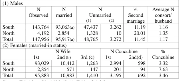
being a wife, a succeeding wife (2nd wife, 3rd wife etc.) after the predecessor deceased, or a concubine as listed in panel (2) of Table 1. With these numbers, we may count that 85.5% of women were married as the first wife, 9.8% as the second wife; while those married as the third up to the sixth wife were in small proportion. Besides being married as a wife, some women were married as concubines and they counted for 3.46% among all in-married women.
Table 1: Marital Status of Lineage Members (1) Males N Observed N married N Unmarried (1) (2) % Second marriage Average N consort/ husband South 143,764 93,063(a) 47,437 3,262 11.19 1.16 North 4,192 2,854 1,328 10 20.01 1.35 Total 147,956 95,917(a) 48,765 3,272 11.45 1.17
(2) Females (married-in status) N Wife 1st 2nd (b) 3rd (c) N Concubine 1st 2nd(d) % Concubine South 93,029 10,412 1,263 2,994 598 3.32 North 2,854 571 147 201 94 7.63 Total 95,883 10,983 1,410 3,195 692 3.46
Source: Ts’ui-jung Liu 1992:60-61, Tables 3.1-3.2.
Notes: (1) Including those whose marital status unknown, age at death unknown or below 40. (2) Including those whose age at death above 40.
(a) Including 34 males who are uxorilocally married.
(b) Those whose status is a wife of a man’s first succeeding marriage.
(c) Those whose status is a wife of a man’s second and later succeeding marriages. (d) Those whose status is a concubine other than the first one.
A comparison of the number of 2nd wife and that of married males shows that on the whole, 11.45% (south 11.19%, north 20.01%) of married males had a 2nd wife. A comparison of the number of all consorts and that of married males shows that on the average, there were 1.17 (south 1.16, north 1.35) consorts per husband. These estimates suggest that remarriage was not unusual among the Chinese lineage males. The above estimates reveal a substantial regional difference in respect to remarriage. There is also a difference in the practice of concubinage; the concubines counted for 3.32% in the south and 7.63% in the north. This regional difference was mainly a reflection of the fact that northern families and lineages under studies had a higher social status than southern ones. It is notable that the lineage which witnessed the highest percentage of concubine (35%) was the Wan-p’ing Wang 宛平王 of Hopei.
Nevertheless, concubinage must not be taken for a prevalent practice in the traditional Chinese society. In general, it is found that a higher percentage of concubine existed in a lineage containing a higher proportion of males belonging to
4
the class of gentry and in a lineage residing in urban area.8 After all, both the gentry and the urban-dweller were just the minority among the Chinese population in the past. For the majority, monogamy rather than concubinage was the norm.
As for the remarriage of women, the genealogies did not have a consistent way of recording. The available data show that the highest percentage of women remarried out was 8.6% and the lineage which had records of remarried women was not limited to one province. As mentioned above, more than ten percent of married males got a second wife and the sex ratio was not balance, therefore, there was indeed a demand for re-marriageable women in the marriage market.
Most of these women got remarried because their husbands died at a young age. In the Ch’ing society, people had different attitudes toward young widows. On the one hand, the state bestowed honor to chaste women and lineages set up charitable estates to support widows and orphans. On the other hand, there were villains seeking every means to force young widows to remarry and thus to obtain profits for themselves. Between these two extremes, the middle-of-the-road was to encourage and support those insisting to keep widowhood and to arrange remarriage for those preferring to marry again. In short, woman’s remarriage in the Ch’ing society reflected not only demographic behavior but also economic and social realities as well as moral and value judgments.9
Besides women who already married into the lineages, there were some being recorded as betrothed or arranged a marriage ceremony after death. The number of these categories is not listed in Table 1. Such information, together with uxorilocal marriage, reveals that men and women in traditional Chinese society had a tendency of getting married by all means. This custom of universal marriage was traditional and exceptions must be only found locally or temporarily in China.10
1.2 Age Difference
With available vital dates we may analyze the age difference between the husband and the consort of various statuses. For this analysis, we use the data of conjugal families instead of the individual persons. It should be noted that the two data sets are quite similar in compositions.11 The advantage of the data set of families
8
Ts’ui-jung Liu 1992:46-47. 9
Ts’ui-jung Liu 1992:48-49; Angela Leung 1992:413-450. 10
Ts’ui-jung Liu 1992:45. 11
The composition of the two data sets may be summarized below: Data set Average N of
consorts % 1st wife % 2nd wife % 3rd wife % concubine Persons 1.22 86.9 9.0 1.0 3.1 Families 1.17 85.5 9.8 1.2 3.5
5
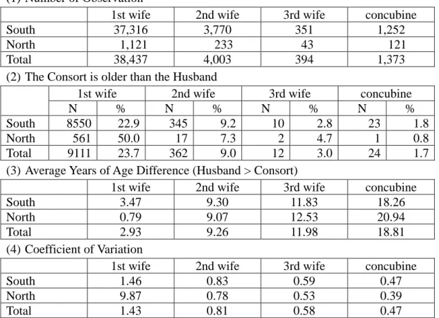
is that it provides more complete vital does then does the one of persons. The statistics of the age difference between the husband and the consort are summarized in Table 2.
Table 2: The Age Difference between Husband and Consort (1) Number of Observation
1st wife 2nd wife 3rd wife concubine
South 37,316 3,770 351 1,252
North 1,121 233 43 121
Total 38,437 4,003 394 1,373
(2) The Consort is older than the Husband
1st wife 2nd wife 3rd wife concubine
N % N % N % N %
South 8550 22.9 345 9.2 10 2.8 23 1.8
North 561 50.0 17 7.3 2 4.7 1 0.8
Total 9111 23.7 362 9.0 12 3.0 24 1.7
(3) Average Years of Age Difference (Husband > Consort)
1st wife 2nd wife 3rd wife concubine
South 3.47 9.30 11.83 18.26
North 0.79 9.07 12.53 20.94
Total 2.93 9.26 11.98 18.81
(4) Coefficient of Variation
1st wife 2nd wife 3rd wife concubine
South 1.46 0.83 0.59 0.47
North 9.87 0.78 0.53 0.39
Total 1.43 0.81 0.58 0.47
Source: Ts’ui-jung Liu 1992:74-78, Tables 3.6-3.8.
It is quite clear that most men did not marry to women of the same age. When we calculate the numbers of consort who were older than their husbands by 0.01 year and more as shown in panel (2) of Table 2, we find on the whole, 23.7% of the 1st wife, 9% of the 2nd wife, 3% of the 3rd wife and 1.7% of the concubine were older than their husbands. These estimates show that the ideal cherished by the ritual and the law that the groom be older than the bride was not always realized.12 As a matter of fact, the result of statistics showed that 50% of the 1st wife in the north was older than the husband; thus a custom in north China to marry older women was well proved.13 Moreover, quite a number of the 2nd and 3rd wife were older than their husbands; this suggests that these women were not married for the first time although the genealogies did not say it clearly.
12 Ch’en Ku-yuan 1975:129.
6
When we calculate the average year of age difference as shown in panel (3) of Table 2, we find on the whole, the husband was older than the 1st wife by 2.93 years, the 2nd wife by 9.26 years, the 3rd wife by 11.98 years, and the concubine by 18.81 years. The age difference became greater with the sequence of succeeding marriage but the variation between the south and the north became smaller. This can be seen from the coefficient of variation listed in panel (4). In other words, there was a wider range of age difference in the first marriage; therefore, the homogeneity of the age of 1st wife was smaller than that of other consorts. This result has two implications. On the one hand, it reflects that there was a tendency of getting married universally regardless whether the age of the couple was match or not. On the other hand, it reflects that the sex ratio was not balance, thus, one had to seek a consort in a wider age range. As for the age difference between the husband and the concubine, the statistical result simply confirms the very nature of this marriage.14
1.3 Situation of Widowhood
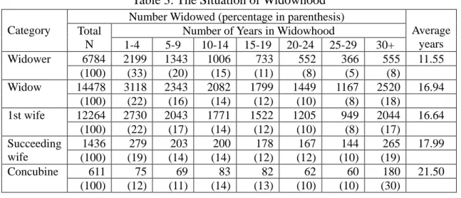
With the reference of vital dates, we may also analyze the situation of widowhood. The statistics are organized for widowers among men who married only once and for widows among all consorts, among the 1st wife, the succeeding wife, and among the concubine as shown in Table 3.
Table 3: The Situation of Widowhood
Category
Number Widowed (percentage in parenthesis)
Average years Total
N
Number of Years in Widowhood
1-4 5-9 10-14 15-19 20-24 25-29 30+ Widower 6784 2199 1343 1006 733 552 366 555 11.55 (100) (33) (20) (15) (11) (8) (5) (8) Widow 14478 3118 2343 2082 1799 1449 1167 2520 16.94 (100) (22) (16) (14) (12) (10) (8) (18) 1st wife 12264 2730 2043 1771 1522 1205 949 2044 16.64 (100) (22) (17) (14) (12) (10) (8) (17) Succeeding wife 1436 279 203 200 178 167 144 265 17.99 (100) (19) (14) (14) (12) (12) (10) (19) Concubine 611 75 69 83 82 62 60 180 21.50 (100) (12) (11) (14) (13) (10) (10) (30)
Source: Ts’ui-jung Liu 1992:79-83, Tables 3.9-3.13.
It should be noted that a calculation of the number widowed as a proportion of the total number in observation in each category showed that 19.1% of the men married once became widowers, 32.7% of all consorts, 31.9% of the 1st wife, 35.9%
14
7
of all succeeding wife, and 44.5% of all concubines became widows.15 From Table 3, we can see that there was a larger percentages of women widowed for more than 15 years. When the percentages widowed for more than 15 years were summed up, they made up 32% of the widower, 48% of the widow, 47% of the 1st wife, 53% of the succeeding wife, and 63% of the concubine. On the average, years of widowhood were 11.55 for the widower, 16.94 for the widow, 16.64 for the 1st wife, 17.99 for the succeeding wife and 21.5 for the concubine. In short, these estimates show that in traditional Chinese society, more women than men remained in widowhood and for a longer duration.
The situation of widowhood can also be analyzed by age distribution. Take the case of 1st wife for example; it is found that 48.29% of them became widows during the childbearing period. When this percentage is multiplied by the proportion widowed among the 1st wife (31.9%), then it shows that 15.4% of the 1st wife was widowed during the childbearing ages. This estimate may serve as a reference for considering the effect of widowhood on fertility.
2. FERTILITY
The data set of reconstituted conjugal families is also used for the analysis of fertility. These families consist of parents and sons (including those died young) but no daughters. Daughters are omitted because their numbers were usually under recorded by the genealogies and their vital dates were not provided. Due to this defect of the data, the fertility can only be estimated in terms of male births in this study. Of the 42,785 conjugal families observed, 42,459 (99%) have complete birth dates of parents; 82% have complete birth dates of all sons; 28% lack father’s death date and 37% lack mother’s death dates. Most of the families consist of sons born by one mother; only 5.7% of the families consist of sons born by two and more mothers. This is the state of incompleteness of the data and some holes can reasonably be amended for the purpose of analysis.16 Using this data set, we may study some aspects related to the fertility of lineage populations.
2.1 Age at Birth of the First Son
We may estimate the age at birth of the first son in order to speculate on the plausible mean age at marriage as the genealogies do not provide record of the date of marriage. Here, the estimates derived from the total number observed and the cohort
15
Ts’ui-jung Liu 1992:54.
8
groups of 1300-1549, 1550-1649, 1650-1749, 1750-1849, and 1850-1899 will be presented. With the total number observed, the average age at birth of the first son for the husband was 27.59 (in south, 28.40; in the north, 25.14) and the average age for the 1st wife was 24.73 (south 24.82; north, 24.37). Among the cohort groups, it is notable that the average age tended to be quite stable when the 1300 and the 1850 groups were not taken into comparison.17
Moreover, the coefficient of variation calculated with the data distributed by age groups shows that it is 0.26 for the husband and 0.24 for the 1st wife; this implies that the variation of the age at birth of first son is not very large. Besides, the mean age and the median age calculated with the age group data show that the latter is lower than the former; this implies that there is a skew to the side of younger age. Thus, it is better to take the median age, 27.36 for the husband and 23.85 for the 1st wife, as a more plausible estimate for the age at birth of first son.18 With these estimates of age at birth of first son, we still have to solve the problem of what is a plausible estimate of the interval between marriage and the birth of first son? To answer this question to some extent, this study tries to estimate the birth intervals. 2.2 The Birth Interval
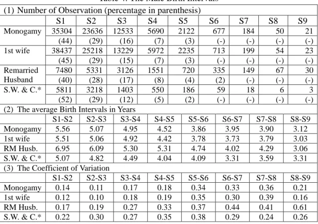
The statistics of male birth intervals are organized for four groups: the monogamy family, the 1st wife, the remarried husband, and the succeeding wife and concubine. These results are summarized in Table 4. Before going on to findings about the birth interval, I should make a few points about the data. First, the monogamy family refers to the family of the husband who married only once; it does not include the family of succeeding marriage which also maintains the state of one husband and one wife. Moreover, the number of S1 listed in Table 4 is identical with the number of observation in each group. It should also be noted that in the case of remarried husband, sons born by consorts of different status are all included and arranged with the birth order according to the father; while in the case of the succeeding wife and concubine, sons are arranged with the birth order according to their own mother.
From Table 4, we see that the distribution of sons by the birth order is actually very similar among the four groups; it is almost identical between the monogamy family and the 1st wife. The distribution also reveals that most of the families had at
17
Some lineages have very small number observed for the 1300 cohort group and thus there is a greater variation among the lineages. The 1850 cohort group consists only 50 years and due to the time limit of the compilation of genealogies, observations of deaths tend to be bias to younger ages. Thus, it is better to take these two cohort groups only for reference but not for serious comparison. 18 Ts’ui-jung Liu 1992:88, 107-109.
9
most three sons. A notable difference exists between the husband married once and the husband remarried; the former had about 10% of sons as the fourth son and above while the later had about 14%. It is also notable that the succeeding wife and concubine had a much larger percentage (52%) of sons born as their own first son and smaller percentage of sons born as their own third son and above.
Table 4: The Male Birth Intervals (1) Number of Observation (percentage in parenthesis)
S1 S2 S3 S4 S5 S6 S7 S8 S9 Monogamy 35304 23636 12533 5690 2122 677 184 50 21 (44) (29) (16) (7) (3) (-) (-) (-) (-) 1st wife 38437 25218 13229 5972 2235 713 199 54 23 (45) (29) (15) (7) (3) (-) (-) (-) (-) Remarried Husband 7480 5331 3126 1551 720 335 149 67 30 (40) (28) (17) (8) (4) (2) (-) (-) (-) S.W. & C.* 5811 3218 1403 550 186 59 18 6 3 (52) (29) (12) (5) (2) (-) (-) (-) (-)
(2) The average Birth Intervals in Years
S1-S2 S2-S3 S3-S4 S4-S5 S5-S6 S6-S7 S7-S8 S8-S9
Monogamy 5.56 5.07 4.95 4.52 3.86 3.95 3.90 3.12
1st wife 5.51 5.06 4.92 4.42 3.78 3.73 3.79 3.03
RM Husb. 6.95 6.09 5.30 5.31 4.74 4.02 4.29 3.06
S.W. & C.* 5.07 4.82 4.49 4.04 4.09 3.31 3.59 3.31
(3) The Coefficient of Variation
S1-S2 S2-S3 S3-S4 S4-S5 S5-S6 S6-S7 S7-S8 S8-S9
Monogamy 0.14 0.11 0.17 0.18 0.34 0.33 0.36 0.21
1st wife 0.12 0.10 0.18 0.19 0.35 0.30 0.39 0.16
RM Husb. 0.17 0.19 0.27 0.33 0.37 0.44 0.41 0.61
S.W. & C.* 0.22 0.30 0.27 0.35 0.38 0.29 0.24 0.26
Source: Ts’ui-jung Liu, 1992:100-117, Tables 4.4-4.7
* For sons of the succeeding wife and concubine, the birth order is arranged according to the mother instead of to the father as in the other groups.
(-) Indicates less than one percent.
The average years of birth intervals, again, reveal a similarity between the monogamy family and the 1st wife. The intervals of S1-S2 and S2-S3 were about 5.5 years, of S3-S4, 5 years, of S4-S5, S5-S6, S6-S7, and S7-S8, 4 years, and of S8-S9, 3 years. Because these estimates were done only with the male births, it is possible that each of the first three intervals was large enough to allow a daughter to be born if these families had daughters. It is reasonable to guess that for parents who already had sons of higher-parity, the possibility of having daughters of higher-parity must be limited. In this case, the intervals of higher-parity tended to be larger than those of lower-parity; this pattern was similar to that found for the pre-1759 European populations.19
19 Flinn 1981:33.
10
Also notable is a deviation in the case of remarried husband. Except for the last interval, the average years for other intervals were longer for the remarried husband than for the monogamy husband. Particularly, the interval S1-S2 was about 7 years and that of S2-S3, 6 years; these estimates imply that an additional time was required for a man to get married again. Moreover, from the individual case rather than from the average, we can see the existence of concubine to cause a birth interval being shorter than normally required.20
As for the succeeding wife and concubine, two different points are notable. Firstly, the birth intervals of their sons were slightly shorter than those of the 1st wife. Secondly, the coefficient of variations was greater. In general, this group of woman had a lower fertility than the 1st wife. From Table 4, we see that the distribution of sons by the birth order is actually very similar among the four groups; it is almost identical between the monogamy family and the 1st wife.
It should be stressed that although the birth intervals are estimated here with the male births only, still the results can be taken as quite plausible. For example, in the case monogamy family, if we suppose that there were daughters born in the first three birth intervals of sons, then, each birth interval would be about 2.5-2.75 years. This length of birth interval was justifiable when the practice of breast feeding was taken into consideration.21 Moreover, the birth interval of such a range was comparable to that of 22.9-31.3 months (1.9-2.6 years) estimated for the 1-2 and 2-3 births for the pre-1750 populations in England and France;22 and to that of 2-4 years found for the populations of Fujito and Fukiage in Japan during the eighteenth and nineteenth centuries.23 For both the European and Japanese cases, scholars attribute high infant mortality as a factor of long birth intervals.
Finally, with the birth interval estimated for S1-S2 as 5.5 years for the monogamy family, we may guess that an interval of 3-5 years may be required between the marriage and the birth of the first son.24 Thus, taking the median age at birth of the first son as a reference, we obtain estimates of age at marriage for the male as 22.36-24.36 and for the female, 18.85-20.83. These estimates, especially the lower ones, are close to those found by other scholars and in records of documents
20 Ts’ui-jung Liu 1992:90.
21 Ts’ui-jung Liu 1992:89-90. 22 Flinn 1981:33.
23 Hanley and Yamamura 1977:241-243. 24
The interval between marriage and first birth (0-1) is estimated as 14.2 months and that between the first and second births (1-2) as 28.4 months for the pre-1750 population of England; the first interval is 16.1 months and the second one is 22.9 months for the pre-1750 population of France. See Flinn 1981:33. Thus, it seems that the interval of 0-1 is at least a half of the interval of 1-2. Since we only have the interval of S1-S2 as a reference, we can only guess that at least half of this time interval is required.
11 other than the genealogies.25
2.3 Marital Fertility Rate
The marital fertility rate can be estimated here only in terms of male births due to the limitation of data. Besides this limitation, for the purpose of estimating age specific fertility rate, there are still two problems to be solved. First, it is the problem of starting the observation. Since the record of age at marriage is missing, it is impossible to start observation from the age at marriage. Though this may be solved by taking an average age, here I simply take the earliest age group, 10-14, in order to include births actually observed for parents at this youngest age group. It should be pointed out, however, even some births are observed with the age groups 10-14 and 15-19, for a strict sense of marital fertility, estimates for these two age groups should not be included for the husband. Second, it is the problem of ending the observation. For most of the cases in which the parents’ death dates are available, the ending of marriage can be easily determined. Otherwise, the age at birth of the last son is taking as a reference.26
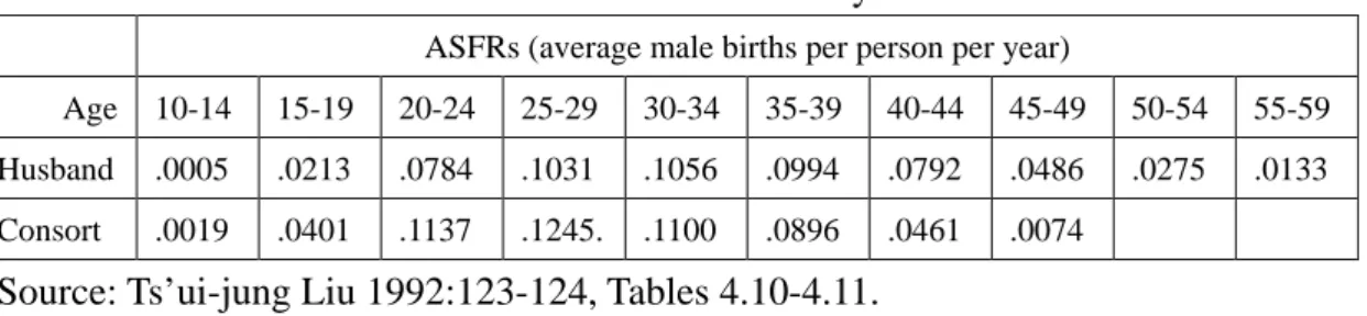
Estimates of the age specific marital fertility rate in terms of male births (denoted as ASFRs) and the total fertility rate (TFs) derived by a summation of ASFRs times five are done for the husband and the consort of 50 lineages. The averages of 50 lineages are listed in Table 5.
Table 5: The Marital Fertility Rate
ASFRs (average male births per person per year)
Age 10-14 15-19 20-24 25-29 30-34 35-39 40-44 45-49 50-54 55-59 Husband .0005 .0213 .0784 .1031 .1056 .0994 .0792 .0486 .0275 .0133 Consort .0019 .0401 .1137 .1245. .1100 .0896 .0461 .0074
Source: Ts’ui-jung Liu 1992:123-124, Tables 4.10-4.11.
We can see that the peak of ASFRs for the husband was at age group 30-34 and for the consort at 25-29. Among the 50 lineages, 24 had the same peak for the husband and 34 the same peak for the consort. Values of ASFRs to the right and left of the peak were actually very close to that of the peak and there was no sharp decline afterwards; this kind of fertility pattern was similar to the one of natural fertility. If we take ages 20-59 for the husband and 15-49 for the consort to calculate the
25
Ts’ui-jung Liu 1992:55. Compared with the preindustrial Japan, the age at marriage estimated for Chinese population is about 4 years lower. See Susan Hanley and Kozo Yamamura 1977: 246-247; Akira Hayami 1985:125, Table 5.11.
26
12
TFs, we obtain 2.78 for the husband and 2.65 for the consort. The difference between the husband and the consort was mainly due to the effect of remarriage.27 From the TFs of husband estimated for individual lineage, we can see that the highest TFs (3.5) was found in Taiwan,28 the next highest (3.0) was in Hunan and Hupei, the lowest (2-2.5) was in Kiangsu, and the middle (2.5-3) was in other provinces.29
In addition to the above estimates showing the result of average, a few words may be added to describe the situation of deviation. It is notable that among the 50 lineages, 25 had the husband and 39 had the consort who gave male birth at ages 10-14. The number counted 107 for husbands (0.25%) and 370 for consorts (0.8%). These numbers give us some ideas about the occurrence of extremely early marriage in the traditional society. Moreover, it is notable that 39 lineages had the husband who had sons born at age above 60 and 42 lineages had the consort who gave male births at age above 45. Although fertility rate at these high ages was rather low, this deviation still reveals that it was desirable to have a son born even when one was already in old age for it was important to continue the family line.30
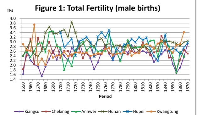
In order to investigate changes of fertility through time, the data of the husband belonging to lineages from the same province are pooled together for estimates of 5-year cohort groups and periods. The ASFRs of each 5-year cohort groups are first calculated and then the values at 8 age groups (20-59) of 8 cohort groups are summed up for the TFs of a corresponding period. To save the space, estimates of cohort ASFRs are omitted here. It should be noted, however, estimates of ASFRs by cohort groups revealed that the peak and the shape of fertility curve were similar among cohorts. In other words, the age pattern of fertility did not change in the long term. As for the TFs, distributions of six provinces are depicted in Figure 1.
Figure 1 shows that estimated values of the TFs fall mostly between 2.4 and 2.8; in other words, the estimates for lineages observed in each province tend to be around the average value. Thus, we should try to find out periods with exceptional high or low TFs and see shy did these exceptions occur. We can find that some short term fluctuations of the TFs took place in periods when natural calamities, such as flood, drought, famine and epidemic disease, occurred and in the period of Taiping
27
Take the ratio of husband’s fertility over consort’s fertility as a dependent variable, the average number of consort per husband as an independent variable, and use the data of 50 lineages in an ordinary least square regression, the result shows that the independent variable is indeed related to the dependable variable and the adjusted R square is 0.67. See Ts’ui-jung Liu 1991: 94.
28
The TFs estimated for consorts of the Yu lineage is 3.38. If we take sex ratio at birth to be 106, then we obtain an estimate of total fertility as 6.69. The total martial fertility rate estimated for Hai-shan during 1906-1930 ranged between 6.15 and 7.08; see Arthur P. Wolf 1985:169, Table 7.7. Since members of the Yu lineage observed were born mostly in the eighteenth and nineteenth centuries, it seems that the martial fertility rate in Taiwan remained quite high and stable since the eighteenth century.
29 Ts’ui-jung Liu 1992:94-95. 30 Ts’ui-jung Liu 1992:92-93.
13
Rebellion. Periods of low TFs concurrent with notable events of calamities in each province are as follows:31
In Kiangsu: 1665-89, 1705-14, 1745-54, 1770-4, 1781-4, 1825-34, 1855-64; In Chekiang: 1665-9, 1745-59, 1820-9, 1845-64; In Anhwei: 1705-19, 1780-4, 1830-4, 1850-9; In Hunan: 1665-74, 1745-9, 1770-89, 1805-30, 1850-64; In Hupei: 1720-4, 1745-9, 1770-4, 1825-34, 1845-59, 1860-4; In Kwangtung: 1690-1704, 1740-9, 1795-1809, 1850-4.
The above list suggests that although some fluctuations were particular for individual province, some were common for different provinces. For instance, a common bad time induced by natural calamities was found around 1710 for Kiangsu and Anhwei, around 1740-50 for Kiangsu, Chekiang, Hunan and Hupei; around 1820-30 for Kiangsu, Chekiang, Anhwei, Hunan and Hupei; and a common crisis due to the Taiping Rebellion was found around 1850-60 for all provinces concerned. Besides the periods of exceptional low TFs, some periods of high TFs are also notable. A few examples should be enough to show the behavior of people during a
31
The records of natural calamities are mainly found in the local gazetteers. The counties concerned are Wu-chin 武進, Chiang-tu 江都, Chiang-yin 江陰, and Tan-t’u 丹徒 in Kiangsu; Hsiao-shan 蕭山 and Yu-yao 餘姚 in Chekiang; T’ung-ch’eng 桐城 and Hsiu-ning 休寧 in Anhwei; Heng-yang 衡陽, Ch’ing-ch’uan 清泉 and Shao-yang 邵陽 in Hunan; Wu-ch’ang 武昌 and Ch’i-shui 蘄水 in Hupei; Hsiang-shan 香山, Hsin-hui 新會, Nan-hai 南海, and P’an-yu 番禺 in Kwangtugn. For details of reference, see Ts’ui-jung Liu 1992:102.
1.4 1.6 1.8 2.0 2.2 2.4 2.6 2.8 3.0 3.2 3.4 3.6 3.8 4.0 16 50 16 60 16 70 16 80 16 90 17 00 17 10 17 20 17 30 17 40 17 50 17 60 17 70 17 80 17 90 18 00 18 10 18 20 18 30 18 40 18 50 18 60 18 70 TFs Period
Figure 1: Total Fertility (male births)
14
time of recovery. In Kiangsu, the TFs reached 3.0 only in the period 1725-9, which included the ASFRs of cohorts of 1670-1709; this reflected a high fertility in a time of rest after disturbances in the lower Yangtze area (Chiang-nan 江南) in early Ch’ing. This peak of TFs in Kiangsu was especially remarkable in comparing with a generally lower level of TFs around 2.0 estimated for the period from 1650 to 1680 when quite a number of natural calamities took place in counties concerned. In Anhwei, the peak of TFs (3.4) was found in periods 1685-9 and 1690-4 with the peak values of ASFRs of cohorts 1660, 1665, and 1670. In Kwangtung, a peak of TFs (3.7) was found in period 1665-9 which included three peak ASFRs of cohorts 1630, 1635 and 1640 then at ages 25-39. It is quite revealing that these cohorts might have taken the best chance right after the establishment of the Ch’ing dynasty to do their reproduction. Again, the high TFs value in period 1865-9 in Kwangtung was also made possible by peaks of ASFRs of three cohorts. Moreover, in Hunan, a consecutive high level of TFs value was found in 1680-1724 with an average of the 9 periods counted as 3.5; apparently, the Hunan lineages concerned were growing most rapidly during these 45 years when the time was peaceful and there was no disturbing natural calamity.
In short, the estimated values of TFs by periods revealed that short term fluctuations were concurrent with crises induced by natural and artificial calamities. Due to a lack of the measurement for the factor induced by calamities, however, a correlation between the fertility and this factor is still to be found. It is notable that the fertility tended to recover soon after short term crises, especially remarkable was that even after the Taiping Rebellion, in 1870-4, the TFs showed a recovery in most provinces concerned. As for the long term trend of TFs, estimates of periods 1550-1649 for Anhwei and Hunan reveal that the fertility was lower in late Ming than in Ch’ing. Estimates for six provinces show that the level of TFs was much higher in the period around 1675-1725 then before the 1670s; after the 1730s until around 1850, the fertility level remained quite stable but not as high as before. With the estimates now available we can mark out the time around 1675-1725 as a high fertility period and this provided the demographic condition backing up the K’ang-hsi Emperor’s 1712 edit, which ordered that no tax should be added to the increasing number of newly born males during the Dynasty’s prime time of prosperity.
It should be mentioned by passing that the TFs obtained by summing up the ASFRs is usually higher than the value calculated by simply taking the average number of sons per father. When the observation is made with the father died above age 50, it is found that on the average, each father had 2.29 sons, only about 82% of the average TFS (2.78). This difference is mainly due to the fact that in the calculation of simple average, fathers who had no son are also included. On the whole, it was found that about 10.4% of the father died above age 50 and 21% among all fathers
15
were sonless.32 Moreover, although the fertility is estimated with male birth only, when a suitable sex ratio at birth is taken, a total fertility of both sexes can still be derived. For instance, if the sex ratio at birth is 106 and the TFs value is 3.5, then we may obtain a total fertility of 7.21. This suggests that during the crucial period of 1675-1725, the fertility was rather high.
3. MORTALITY
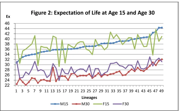
As mentioned in the beginning of this paper, only about 40% of persons observed with birth dates have records of death dates and most of those died below age 15 have no records of vital dates. The defect of the data makes it very difficult to study the child mortality with the genealogies. Thus, only the adult mortality will be discussed here. For the estimation of adult mortality, life tables are constructed for the male and the female of each lineage. To save the space, only estimates of the expectation of life (Ex) at age 15 and 30 are depicted in Figure 2.
Figure 2 is arranged with an ascending order of the life expectancy at age 15 (E15) of males. It should be noted that although the number observed in each lineage varies, this variation is not the main reason for the variations of estimated Ex. Moreover, most lineages have more than 50% of persons observed with age at death known. Thus, though the data are not complete, they are still quite useful for the estimation of adult mortality.33
From Figure 2, we obtain an impression that the order of lineages varies between ages and sexes. At age 15, the average years of life expectancy of males range from 32.96 (Yu游of Taiwan) to 44.4 (Sung宋of Henan and Lao勞 of Shantung); those of females from 29.3 (Wang王 of Hopei) to 43.6 (Shao-yang Li 邵陽李of Hunan). At age 30, the average years of life expectancy of males range from 22.14 (Yen嚴 of Chekiang) to 32.07 (Lao勞 of Shantung); those of females from 23.87 (Wang王 of Hopei) to 33.04 (Ch’ien錢 of Chekiang). These values at the two extremes are comparable with the model west life table levels 1 to 12.34 The difference is indeed in a wide range. However, most of the lineages fell in the middle instead of in the extremes. Take the E15 for example, the males of 26 lineages (from number 8 to 33) have the values comparable with the west model levels 5-8 (35.27-39.19); the females of 30 lineages have the values comparable to the same levels (37.07-41.24). The difference between the male and the female can also be seen
32 Ts’ui-jung Liu 1992: 98-99. 33
A polynomial regression equation is applied to adjust the Qx values calculated with the observed data and the results show that for the male, only 7 lineages have the coefficient of determination less than 0.9 while for the female, there are 21 lineages. See Ts’ui-jung Liu 1992:139. Thus, the data of the female are not as good as those of the male.
16
from Figure 2. At age 15, there are 17 estimates of the female falling below that of the male; at age 30, there are only 3. This seems to imply that at younger ages of reproduction, there is a greater risk of death for the female.
When we plot the Qx (the probability of dying at age x) of the male of selected lineages with that of a certain level of west model as shown in figures 3-6, we can see that most of the lineages have a higher Qx at age 45 and above.
22 24 26 28 30 32 34 36 38 40 42 44 46 1 3 5 7 9 11 13 15 17 19 21 23 25 27 29 31 33 35 37 39 41 43 45 47 49 Ex Lineages
Figure 2: Expectation of Life at Age 15 and Age 30
M15 M30 F15 F30 0.0 0.2 0.4 0.6 0.8 1.0 15 20 25 30 35 40 45 50 55 60 65 70 75 80 Qx Age
Figure 3: Qx (1)
17 0.0 0.2 0.4 0.6 0.8 1.0 15 20 25 30 35 40 45 50 55 60 65 70 75 80 Qx Age
Figure 4: Qx (2)
Wei CcLi SyLi West 8
0.0 0.2 0.4 0.6 0.8 1.0 15 20 25 30 35 40 45 50 55 60 65 70 75 80 Qx Age
Figure 5: Qx (3)
HsHsu YcCheng Yu West 5
0.0 0.2 0.4 0.6 0.8 1.0 15 20 25 30 35 40 45 50 55 60 65 70 75 80 Qx Age
Figure 6: Qx (4)
18
This finding confirms with the “Far Eastern Pattern of Mortality” found by Goldman.35 Also, it is notable that the curve of the Huang黃 Lineage in Kiangsi is almost identical with that of the west model level 6 (Figure 3) and the curve of three lineages in Hunan are very close to that of the west model level 8 (Figure 4). These cases reveal that with a large enough number in observation, the estimates of mortality can still be quite plausible with the genealogical data.
The above estimates of the adult mortality based on the data of individual lineages may reflect the well-being of the lineages to some extent. For example, the estimates of Ex for both males and females of the three lineages in Hunan were commonly comparable with the west model level 8. The settlements in which these three lineages resided were around the Hsiang湘 and Tzu資 Rivers with abundant agricultural resources which were developed during the Ming and Ch’ing periods.36 The low mortality of these three lineages can be more reasonably conceived under this economic condition. Moreover, some northern lineages under studies also have higher estimates of the Ex; this may be related to the fact that they had a higher social status and a better livelihood. However, it is notable that the Ex of the female of Wan-p’ing Wang in Hopei was the lowest among all lineages under studied. As mentioned before, the Wan-p’ing Wang was a family with high social status; 48% of its males held degrees or titles and most of its daughter-in-law came from families of comparable status, but why did these women brought up delicately die much younger than other common women? Perhaps, this special case can be approached with the fact that this Wang lineage also had the largest proportion of concubine (35%) among its in-married women. Did polygamy have any relation to the high mortality of these women? This is still a puzzle.
We can also compare the estimates of this study with those derived by other scholars. The life tables constructed with the data of a genealogy of Kwangtung by I-chin Yuan provide an average of E20 for the males of cohorts 1365-1849 as 35.1 years.37 The five Kwangtung lineages in this study show the estimates of E20 are 35.05, 35.04, 34.23, 32.30, and 30.81 years; these are not exactly the same but close to Yuan’s estimate. Harriet Zurndorfer provides an estimate of E20 for the Hsiu-ning Fan休寧范 lineage males born in 1500-99 as 42.13 years.38 An estimate of E20 of the same cohorts of Hsiu-ning Chu休寧朱 males was 39.31 years.39 Moreover, the estimates derived by the Princeton demographers show that in the early twentieth century, the Ex of Chinese females was higher in the north than in the south: the E15 35 Goldman 1980. 36 Perdue 1987:25-135. 37 Yuan 1931:167-169. 38 Zurndorfer 1989:182-191. 39 Ts’ui-jung Liu 1992:141.
19
of males in north was 36.9 and in south 29.0 years; the E15 of females in north was 33.5 and in south 28.6 years.40 The estimates of this study also reveal a higher Ex in the north than in the south. But the values estimated by this study are comparable to the model west levels 5-7 while those in the early twentieth century are comparable to level 3. Does this really imply that the mortality of Chinese population was higher in the early twentieth century? If the mortality was becoming higher, when was the possible time?
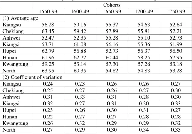
These problems apparently cannot be solved easily with the data we have now. For investigating changes of mortality through time, I have tried to calculate average age at death for the males died above age 15 by cohort groups for various provinces. Due to the nature of genealogical records, cohorts tended to bias to high as low age at death are omitted. Here only cohorts from 1550 to 1799 are taken for comparison. The results are listed in Table 6 by grouping into five broad 50-year cohorts.
Table 6: Average Age at Death of the Male died above Age 15 Cohorts 1550-99 1600-49 1650-99 1700-49 1750-99 (1) Average age Kiangsu 56.28 59.16 55.37 54.63 52.64 Chekiang 63.45 59.42 57.89 55.81 52.21 Anhwei 52.47 52.35 55.28 55.10 52.73 Kiangsi 53.71 61.08 56.16 55.36 51.99 Hupei 62.79 56.88 52.73 56.37 56.50 Hunan 61.96 62.72 60.44 58.25 57.95 Kwangtung 59.25 53.14 57.30 57.26 53.18 North 63.95 60.35 54.82 54.83 53.28 (2) Coefficient of variation Kiangsu 0.24 0.23 0.26 0.26 0.27 Chekiang 0.25 0.27 0.26 0.27 0.30 Anhwei 0.31 0.33 0.31 0.28 0.30 Kiangsi 0.32 0.27 0.31 0.30 0.33 Hupei 0.23 0.26 0.30 0.31 0.27 Hunan 0.22 0.27 0.27 0.28 0.28 Kwangtung 0.26 0.32 0.29 0.29 0.32 North 0.27 0.29 0.30 0.34 0.33
Source: Ts’ui-jung Liu 1992:182-189; Table 5.3.
It should be pointed out that among the cohort groups listed in Table 6, only 5 groups (the 1650-99 of Anhwei, the 1550-99 and 1600-49 of Kiangsi, the 1700-49 of Hupei, and the 1750-99 of North) had the percentage of age unknown higher than 50%. In other words, the data used here are at least good enough for 50% of the
20
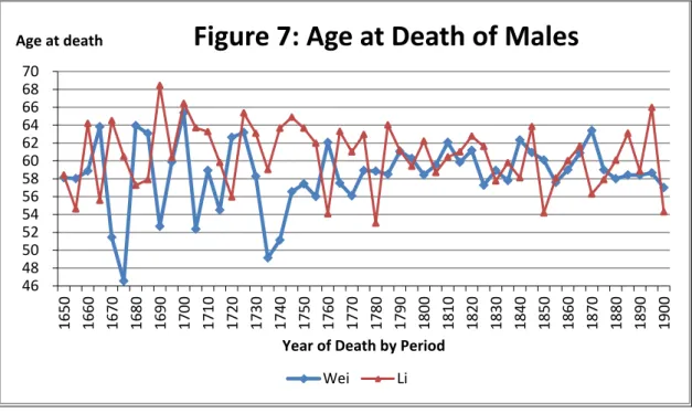
populations under studied. From Table 6, we can see that the coefficient of variation of all groups were about the same, while the average age at death was the lowest for the cohorts 1750-99 in almost every local region. This finding of a lower age at death (a higher mortality) for the cohorts 1750-99 was coincident with the aforementioned increasing unmarried rate and the declining fertility rate. The time was just at the juncture when the Ch’ing dynasty was gradually in decline. These findings should not be overstated, but it is remarkable that changes in demographic phenomena of marriage, fertility and mortality among the lineage populations could be a coincidence with a general decline of the Ch’ing dynasty under which these people lived. It should be noted that the mortality, just as the fertility, fluctuated rather than maintained stably. Due to the fact that the data of deaths are not as complete as those of births, detail statistics have not yet organized by 5-year cohort groups as have been done for the fertility. Here, the Wei and Li lineages of Heng-yang, Hunan, are taken for example.41 Take the year of death as a reference, the males died at age 15 and above are organized by 5-year period and the average age at death is calculated. The results are depicted in Figure 7.
With the reference of events of natural calamities recorded in the 1872 edition of Heng-yang county gazetteer, we can identify some low estimates of average age at death in periods 1705-19, 1730-4, 1745-54, 1825-39, and 1850-69. It is notable that the two lineages showed similar fluctuations in most of these periods. Except for
41
The Li lineage in Ch’ing-ch’uan County, situating to the east of Heng-yang was combined with Heng-yang County in the Republican period.
46 48 50 52 54 56 58 60 62 64 66 68 70 16 50 16 60 16 70 16 80 16 90 17 00 17 10 17 20 17 30 17 40 17 50 17 60 17 70 17 80 17 90 18 00 18 10 18 20 18 30 18 40 18 50 18 60 18 70 18 80 18 90 19 00 Age at death
Year of Death by Period
Figure 7: Age at Death of Males
21
drastic fluctuations caused by the small number observed in the early periods, the concurrence of low age at death with recorded events of natural calamities is still quite instructive for us to understand the nature of fluctuations of mortality in the agricultural China.
4. GROWTH OF LINEAGE POPULATION
The growth of a lineage population can be investigated by estimating the male population with the number of male births in each 5-year interval and a set of survival ratios at different age groups. Through this calculation, we can obtain the estimated male population of a lineage with age structure in each 5-year period. With the estimates of 49 lineages, a few points about the growth of lineage male population may be summarized below.42
(1) The curve of the lineage male population mostly showed a growth trend and the peaks mostly occurred in periods close to the time when the genealogies were compiled: 15 lineages around 1840-55, 10 around 1870-99, and 5 around 1820-25. The cases of exception were found either because there was a large number of out-migration and thus birth dates of emigrants were missing or simply because records of birth dates were missing in a certain section of the genealogy.
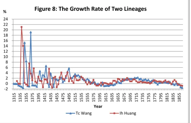
(2) In the early stage of growth process of lineage populations, because the number of males was still very small the growth rate tended to change drastically. Once the male population of a lineage reached a certain number, drastic changes disappeared and the tempos of different lineages could be more or less the same. This can be seen from Figure 8 which shows the examples of the I-huang Huang 宜黃黃 lineage of Kiangsi and the T’ung-ch’eng Wang 桐城王 lineage of Anhwei. It is notable that the curves of growth rate of these two lineages clearly revealed a lower level around 1590-1665 and a higher level around 1665-1765; a remarkable difference between the time of the Ming-Ch’ing transition and that of High Ch’ing could thus be clearly conceived.
(3) Along with the growth of population, the age structure among the lineage males also gradually changes from one with a large proportion at younger ages to one with a large proportion at ages 15-64, that is, the dependency ratio became less than one. Only when this stage of favorable age structure was reached, could a lineage then start to perform its socio-economic functions vigorously.43
In addition to the growth dynamics, we can also estimate the intrinsic growth rate of the lineage population. Here the ASFRs estimated for each lineage and suitable
42 Ts’ui-jung Liu 1992:236-244. 43
22
west model life table are taken as constant to calculate the intrinsic growth rate (IGR). The results show that 12 lineages had estimates of IGR higher than 1%. These lineages had a high IGR because they had comparatively higher fertility and lower mortality. There were 8 lineages whose IGR was negative or close to zero. These lineages had a low IGR because they either had rather low fertility or rather high mortality. For the rest of 29 lineages, the IGR ranged between 0.1% and 0.9%. When the mortality of west model level 6 is used to calculate with the average ASFRs, we obtain the intrinsic growth rate as 0.7% and the length of generation as 32.78 years. This kind of momentum should be quite close to the fact of population growth in China during the period from the late seventeenth to the late eighteenth centuries.
CONCLUSION
This study demonstrates that Chinese genealogies which keep vital records of family and lineage members to some extent can be quite useful for the study of historical demography. With the vital statistics organized from the genealogies, we can investigate into marriage, fertility, mortality, and growth of the lineage populations; the demographic system of Chinese population in the past can thus be grasped to some extent. It is found that these lineage populations tend to marry early and universally; remarriage is not unusual among men and even though the state and the society foster chastity, there is a demand for re-marriageable women; still there are
-20 2 4 6 8 10 12 14 16 18 20 22 24 13 15 13 35 13 55 13 75 13 95 14 15 14 35 14 55 14 75 14 95 15 15 15 35 15 55 15 75 15 95 16 15 16 35 16 55 16 75 16 95 17 15 17 35 17 55 17 75 17 95 18 15 18 35 18 55 % Year
Figure 8: The Growth Rate of Two Lineages
23
more widows than widowers. It is quite clear that the age pattern of fertility does not change in a long time; each conjugal family on the average has 2.5 to 3 sons; the fertility rate varies among provinces and periods, but a generally higher fertility rate can be marked out around the period 1675-1725. The estimates of expectation of life for the lineage adult males and females are mostly comparable to the west model levels 5-7. It is notable that short term fluctuations of fertility and mortality are concurrent with major events of wars and natural calamities. It is also notable that at the juncture when the Ch’ing dynasty starts to decline from its prime time in the late eighteenth century, the demographic system shows a higher percentage celibate males aged 40 and above, a lower fertility rate, and perhaps a higher mortality rate. When the mortality of west model level 6 and the average age specific fertility rate in terms of male births of 50 lineages are taken to calculate the intrinsic growth rate, the result is 0.7%. This momentum of growth is quite plausible in reflecting a doubling of population in China during the period from the late seventeenth to the late eighteenth centuries.
REFERENCES
Barclay, George, Ansley Coale, Michael Stoto, and T. Trussell, “A Reassessment of the Demography of Traditional Rural China,” Population Index, 42.4 (1976), pp. 606-635.
Ch’en Ku-yuan, Chung-kuo hun-yin shih (A history of marriage in China). Taipei: The Commercial Press, 1975.
Coale, Ansley and Paul Demeny, Regional Model Life Table and Stable Population. Princeton: Princeton University Press, 1965.
Ebrey, Patricia Buckley and James L. Watson eds., Kinship Organization in Late
Imperial China, 1000-1940. Berkeley: University of California Press, 1986.
Flinn, Michael, The European Demographic System, 1500-1820. The Johns Hopkins University Press, 1981.
Goldman, Noreen, “Far Eastern Pattern of Mortality,” Population Studies, 34.1 (1980), pp. 5-17.
Hajnal, J., “European Marriage Pattern in Perspective,” in D. V. Glass and D. E. C. Eversley eds., Population in History: Essays in Historical Demography. London, 1965, pp. 101-143.
Hanley, Susan B. and Kuzo Yamamura, Economic and Demographic Change in
24
Hayami, Akira, “Rural Migration and Fertility in Tokugawa Japan: the Village of Nishijo, 1773-1868,” in Susan B. Hanley and Arthur P; Wolf eds., Family and
Population in East Asian History. Stanford: Stanford University Press, 1985, pp.
110-132.
Leung, Angela Ki Che, “To Chasten the Society: The development of Widow Homes in the Ch’ing, 1773-1911,” in Family Process and Political Process in Modern
Chinese History. Taipei: Institute of Modern History, Academia Sinica, 1992, pp.
413-450.
Liu, Ts’ui-jung 劉翠溶, Ming-Ch’ing shih-ch’i chia-tsu jen-k’ou yu she-hui ching-chi
pien-ch’ien 明 清 時 期 家 族 人 口 與 社 會 經 濟 變 遷 (Lineage Population and
Socio-economic Changes in the Ming-Ch’ing Periods). Taipei: The Institute of Economics, Academia Sinica, 1992.
Perdue, Peter, Exhausting the Earth: State and Peasant in Hunan, 1500-1850. Cambridge, Massachusetts: Council on East Asian Studies, Harvard University, 1987. Rozman, Gilbert, Population and Marketing Settlements in Ch’ing China. Cambridge: Cambridge University Press, 1982.
Wolf, Arthur P., “Fertility in Prerevolutionary Rural China,” in Susan B. Hanley and Arthur P. Wolf eds., Family and Population in East Asian History. Stanford: Stanford University Press, 1985, pp. 154-185.
Yuan I-chin, “Life Tables for a Southern Chinese Family from 1365 to 1849,” Human
Biology, 3.2 (1931), pp. 157-179.
Zurndorfer, Harriet, Change and Continuity in Chinese Local History: The
25
APPENDIX: Statistics for Figures 1-8
Table A1: Total Fertility of Lineages grouped by Province
Period Kiangsu Chekinag Anhwei Hunan Hupei Kwangtung
1650 1.62 1.83 2.42 2.40 2.90 1655 2.65 2.42 2.59 2.72 2.65 1660 2.21 3.13 2.35 3.04 2.62 1665 2.03 2.04 2.61 2.46 3.74 1670 1.94 3.17 2.93 2.39 2.02 1675 1.53 2.69 2.97 2.61 2.29 1680 1.94 2.70 2.56 3.41 2.02 1685 2.27 3.00 3.42 3.65 2.63 1690 2.63 2.51 3.46 3.35 2.33 1695 2.23 2.87 2.83 3.35 2.42 1700 2.68 2.32 2.74 3.46 3.40 2.41 1705 2.41 2.61 1.81 3.52 2.77 2.56 1710 2.19 2.61 2.26 3.19 2.93 2.39 1715 2.74 2.38 1.98 3.86 3.13 2.46 1720 2.56 2.57 2.66 3.41 2.41 2.55 1725 3.00 2.73 2.87 2.77 3.02 2.54 1730 2.50 2.29 3.02 2.92 3.10 2.51 1735 2.52 2.66 2.60 3.09 3.21 2.54 1740 2.30 2.77 2.83 2.93 2.98 2.39 1745 1.83 2.37 2.77 2.82 2.38 2.46 1750 2.12 2.48 2.59 3.07 3.22 2.52 1755 2.57 2.47 2.64 3.14 3.40 2.51 1760 2.85 2.79 2.61 2.84 3.20 2.70 1765 2.49 2.52 3.33 2.93 3.50 2.74 1770 2.21 2.46 2.92 2.78 2.24 2.42 1775 2.57 2.60 2.56 2.86 2.73 2.49 1780 2.21 2.85 2.18 2.82 2.52 2.51 1785 2.66 2.51 2.60 2.78 2.90 2.56 1790 2.52 2.46 3.09 3.01 2.90 2.86 1795 2.85 2.60 2.76 2.68 3.12 2.41 1800 2.53 2.51 2.76 2.81 2.99 2.52 1805 2.53 2.63 2.78 2.59 3.20 2.51 1810 2.61 2.98 2.79 2.79 3.08 2.86 1815 2.54 2.69 2.91 2.77 3.17 2.90 1820 2.53 2.42 3.06 2.57 2.71 2.84 1825 2.14 2.55 3.07 2.70 2.39 2.72 1830 2.36 2.60 2.35 2.69 2.19 2.93 1835 2.47 3.26 2.94 3.08 2.62 3.04 1840 2.65 2.98 3.06 3.02 3.30 2.90 1845 2.64 2.33 2.83 3.02 2.59 2.69 1850 2.06 2.32 2.36 2.98 2.73 2.54 1855 1.68 1.81 1.70 2.93 2.65 2.85 1860 1.90 2.24 2.58 2.83 2.47 2.90 1865 2.37 2.66 2.38 2.98 2.76 3.41 1870 2.92 2.50 3.04 2.96
26
Table A2: Expectation of Life at Age 15 and 30
Lineages Male Female Lineages Male Female
M15 M30 F15 F30 M15 M30 F15 F30
1 Wu-chin Liu 30.72 22.47 38.09 31.31 26 Yin-hsien Li 37.15 24.85 33.93 24.98
2 Hsiao-shan Fu 32.12 24.67 30.52 24.85 27T'ung-ch'eng Wang 37.21 25.64 39.83 28.50
3 Taiwan Yu 32.96 23.23 35.36 25.04 28 Hisu-ning Chu 37.70 26.74 37.32 28.48
4 Ch'ing-hsi Yen 33.44 22.14 36.04 27.18 29 Wu-chin Chou 38.16 25.35 37.46 25.76
5 Chiang-yin Miao 33.66 23.24 37.07 26.21 30Hsiao-shan Ts'ao 38.27 26.20 35.77 26.76
6 Hsiang-shan Mai 33.96 24.84 38.03 28.34 31 Hsiao-shan Sihi 38.30 25.92 36.83 27.32
7 Yung-ch'un Cheng 34.06 24.60 41.27 31.29 32 Wu-ch'ang Hsu 38.31 26.34 42.66 30.49
8 Nan-hsun Chou 34.50 22.94 29.65 27.58 33 P'an-yu Ling 38.41 26.52 40.24 30.55
9 Hsiao-shan Hsu 34.89 24.02 37.13 28.08 34 Nan-ch'ang Li 38.79 27.10 41.67 30.94
10 Yu-yao Shih 35.04 24.18 36.75 27.54 35 Hsin-hui Yi 39.14 27.45 39.99 29.65
11 Wu-hin Tsou 35.28 23.73 36.68 25.01 36 T'ien-chin Li 39.14 25.91 37.82 29.36
12 K'uai-chi Ch'in 35.36 23.63 35.34 26.10 37 T'ien-chin Kuo 39.20 26.04 39.10 28.52
13 Nan-ch'ang Kan 35.76 28.85 41.07 30.40 38 Nan-hai Huang 39.25 27.22 40.47 29.92
14 Wu-chin Sheng 35.82 23.60 40.52 28.65 39 Heng-yang Wei 39.83 28.21 40.41 29.80
15Wan-p'ing Wang 35.87 25.41 29.30 23.87 40 Hsiao-shan Lang 39.95 27.49 36.06 27.95
16 Hsiang-shan Hsu 35.91 25.59 39.59 28.51 41 Ch'ing-ch'uan Li 40.18 28.83 41.69 31.55 17 Shang-ch'iu Sung 36.02 25.48 30.65 26.65 42 Cheng-chiang Chang 40.37 27.83 39.43 28.59
18 Chiang-tu Chu 36.06 24.05 37.90 26.45 43 Hsiao-shan Li 40.56 27.51 37.01 28.32
19 I-huang Huang 36.06 26.39 37.11 29.16 44 Hui-min Li 40.67 28.40 37.11 28.98
20Chiang-yin Ma 36.19 26.71 36.53 26.66 45 T'zu-hsi Ch'ien 40.85 29.54 41.88 33.04
21 T'ung-ch'eng Chao 36.31 25.40 38.28 27.87 46 Huang-hsien Ting 42.42 30.87 33.75 29.52
22 I-hsing Cheng 36.61 25.76 38.90 28.36 47 Sho-yang Li 42.76 29.80 43.61 31.51
23 Ch'i-shui Pi 36.89 25.80 38.83 28.27 48 K'ai-feng Sung 44.35 31.53 39.06 32.55
24Hsiao-shan Shen 37.12 25.74 36.01 27.21 49 Hsin-yang Lao 44.36 32.07 40.94 31.16
27 Table A3: Qx (1)
Age Ts'ao Chao Huang Pi West 6
15 0.02084 0.03359 0.04772 0.03132 0.04225 20 0.02975 0.04336 0.05538 0.04080 0.05987 25 0.04191 0.05587 0.06496 0.05300 0.06676 30 0.05826 0.07184 0.07703 0.06865 0.07696 35 0.07991 0.09220 0.09234 0.08868 0.09005 40 0.10816 0.11810 0.11191 0.11421 0.10850 45 0.14444 0.15098 0.13709 0.14668 0.12615 50 0.19034 0.19263 0.16978 0.18785 0.15885 55 0.24750 0.24528 0.21255 0.23988 0.19354 60 0.31756 0.31172 0.26900 0.30545 0.25818 65 0.40205 0.39537 0.34416 0.38785 0.33472 70 0.50226 0.50049 0.44511 0.49107 0.44015 75 0.61913 0.63231 0.58195 0.61999 0.57926 80+ 1.00000 1.00000 1.00000 1.00000 1.00000 Table A4: Qx (2)
Age Wei CcLi SyLi West 8
15 0.02505 0.02788 0.01243 0.03548 20 0.03251 0.03460 0.01833 0.05028 25 0.04221 0.04325 0.02669 0.05586 30 0.05482 0.05444 0.03838 0.06432 35 0.07123 0.06899 0.05452 0.07549 40 0.09259 0.08803 0.07649 0.09152 45 0.12041 0.11312 0.10599 0.10787 50 0.15665 0.14636 0.14504 0.13750 55 0.20388 0.19069 0.19605 0.17072 60 0.26546 0.25018 0.26172 0.23049 65 0.34578 0.33049 0.34508 0.30350 70 0.45059 0.43962 0.44938 0.40538 75 0.58741 0.58884 0.57797 0.54103 80+ 1.00000 1.00000 1.00000 1.00000
28 Table A5: Qx (3)
Age HsHsu YcCheng Yu West 5
15 0.03989 0.05153 0.04883 0.04604 20 0.04958 0.06119 0.06092 0.06525 25 0.06168 0.07311 0.07586 0.07287 30 0.07680 0.08787 0.09426 0.08404 35 0.09571 0.10626 0.11688 0.09821 40 0.11937 0.12927 0.14462 0.11803 45 0.14900 0.15823 0.17857 0.13640 50 0.18614 0.19484 0.22003 0.17082 55 0.23274 0.24139 0.27055 0.20633 60 0.29124 0.30087 0.31196 0.27371 65 0.36476 0.37729 0.40464 0.35222 70 0.45722 0.47500 0.49663 0.45965 75 0.57360 0.60418 0.60554 0.60069 80+ 1.00000 1.00000 1.00000 1.00000 Table A6: Qx (4)
Age WpWang TtKuo TtLi Lu West 6
15 0.03915 0.01099 0.01063 0.03567 0.04225 20 0.04831 0.01820 0.01751 0.04376 0.05987 25 0.05990 0.02932 0.02813 0.05410 0.06676 30 0.07461 0.04585 0.04405 0.06737 0.07696 35 0.09336 0.06964 0.06728 0.08453 0.09005 40 0.11737 0.10274 0.10019 0.10686 0.10850 45 0.14825 0.14722 0.14551 0.13610 0.12615 50 0.18812 0.20489 0.20607 0.17464 0.15885 55 0.23984 0.27697 0.28458 0.22578 0.19354 60 0.30719 0.36366 0.38324 0.29409 0.25818 65 0.39529 0.46377 0.50329 0.38595 0.33472 70 0.51103 0.57445 0.64450 0.51029 0.44015 75 0.66374 0.69113 0.80484 0.67977 0.57926 80+ 1.00000 1.00000 1.00000 1.00000 1.00000
29
Table A7: Average Age at Death aged 15 and above
Year D Wei Li Year D Wei Li
1650 58.11 58.40 1780 58.85 53.02 1655 58.02 54.62 1785 58.49 64.02 1660 58.87 64.18 1790 61.06 61.17 1665 63.82 55.57 1795 60.27 59.39 1670 51.44 64.50 1800 58.42 62.21 1675 46.56 60.49 1805 59.54 58.69 1680 63.94 57.26 1810 62.07 60.43 1685 63.07 57.90 1815 59.84 61.01 1690 52.66 68.44 1820 61.18 62.77 1695 59.87 60.37 1825 57.27 61.60 1700 65.39 66.43 1830 58.93 57.75 1705 52.37 63.70 1835 57.79 59.80 1710 58.93 63.26 1840 62.34 58.10 1715 54.49 59.82 1845 60.93 63.84 1720 62.62 55.95 1850 60.09 54.17 1725 63.17 65.36 1855 57.58 58.07 1730 58.27 63.08 1860 58.99 60.02 1735 49.14 59.01 1865 60.89 61.65 1740 51.14 63.64 1870 63.38 56.30 1745 56.55 64.89 1875 59.00 57.89 1750 57.42 63.65 1880 57.99 60.06 1755 56.02 61.98 1885 58.42 63.09 1760 62.06 54.07 1890 58.41 58.85 1765 57.50 63.30 1895 58.65 65.98 1770 56.09 61.01 1900 57.01 54.29 1775 58.93 62.95
30
Table A8: The growth rate of two lineages: T’ung-ch’eng Wang and I-huang Huang Year Tc Wang Ih Huang Year Tc Wang Ih Huang Year Tc Wang Ih Huang
1315 -0.02 1500 2.06 2.16 1685 1.44 2.08 1320 -0.07 1505 2.08 0.97 1690 1.82 1.49 1325 -0.08 0.94 1510 2.77 0.22 1695 1.78 0.84 1330 -0.63 -0.03 1515 3.55 2.79 1700 1.78 0.85 1335 -0.86 -0.12 1520 2.90 1.29 1705 1.75 1.51 1340 -1.17 21.09 1525 3.19 1.22 1710 2.15 1.56 1345 -1.58 14.03 1530 2.63 1.42 1715 2.05 0.90 1350 15.27 0.25 1535 2.42 2.59 1720 2.27 0.49 1355 8.44 -0.30 1540 1.70 2.11 1725 1.58 0.53 1360 -0.87 -0.70 1545 1.32 1.43 1730 1.82 0.78 1365 -0.99 7.48 1550 1.18 0.50 1735 1.19 0.45 1370 19.18 3.75 1555 1.75 -0.28 1740 1.43 0.52 1375 -0.58 1.24 1560 1.31 0.55 1745 1.57 0.45 1380 -0.63 5.67 1565 0.56 -0.12 1750 1.18 0.29 1385 -0.66 0.69 1570 0.19 0.38 1755 1.42 0.38 1390 -1.10 0.28 1575 0.44 1.41 1760 0.66 0.04 1395 2.27 2.61 1580 0.46 -0.24 1765 1.03 0.37 1400 4.67 1.09 1585 -0.47 -0.73 1770 1.36 0.94 1405 1.30 0.89 1590 -0.02 -0.73 1775 0.63 1.25 1410 3.26 -1.38 1595 -0.31 -0.38 1780 0.28 0.93 1415 2.66 1.59 1600 -0.68 0.38 1785 -0.25 0.70 1420 6.60 1.51 1605 0.43 -0.40 1790 0.30 0.82 1425 0.29 0.41 1610 -0.86 0.22 1795 0.45 0.75 1430 -1.12 5.50 1615 -0.80 0.17 1800 0.47 0.43 1435 3.87 -0.33 1620 -0.70 -0.05 1805 0.58 0.79 1440 2.13 -1.51 1625 -0.80 -0.24 1810 0.54 1.23 1445 -1.14 2.17 1630 -0.48 0.12 1815 0.39 0.57 1450 1.86 2.57 1635 -0.32 0.01 1820 0.25 0.75 1455 1.53 -1.35 1640 -0.54 1.06 1825 0.68 0.25 1460 1.25 -0.24 1645 -0.27 1.07 1830 -0.17 -0.16 1465 1.83 2.30 1650 0.19 0.49 1835 -0.08 0.77 1470 2.25 4.13 1655 0.73 1.77 1840 -0.48 1.34 1475 0.61 1.76 1660 0.29 1.56 1845 0.01 0.78 1480 1.17 1.49 1665 0.24 0.96 1850 -0.46 -0.08 1485 2.22 2.80 1670 0.98 1.58 1855 -0.17 -0.45 1490 4.37 4.22 1675 1.61 1.17 1860 -1.30 -0.65 1495 5.72 0.83 1680 1.49 1.51 1865 -1.47 -0.80