Location Choice Patterns of Computer Use in the United States

(1)

Location Choice Patterns of Computer Use in the

United States

Zhixian Yi

Doctoral Candidate,

School of Library and Information Studies,

Texas Woman’s University, U.S.A

E-mail：zhixianyi@mail.twu.edu

Philip Q. Yang, Ph.D.

Professor, Department of Sociology and Social Work,

Texas Woman’s University, U.S.A

E-mail：PYang@mail.twu.edu

Keywords（關鍵詞）： Location Choice（使用地點）

；

Computer Use（電腦使用）

；

Patterns

（選擇模式）

【

Abstract】

There is little research on the patterns of

computer use outside home or work. This

study examines who is more or less likely to

use a computer at a location other than work

or home by using the 2002–2004 General

Social Survey data and logistic regression

analysis. Demographic variables (such as

age, race, marital status, and region),

socioeconomic status (such as education

and family income), self employment, and

satisfaction with financial situation are

significant predictors of computer use at

locations other than home or work; but

occupation and gender make no difference.

The findings will help institutions to provide

computer infrastructure support and services

for customers in public places, and especially

help schools and libraries to improve

computer labs and services.

【摘要】

過去在探討非居家或上班電腦使用地點的研

究微之又微。本文針對

2002-2004 年總體社會

調查資料進行對數回歸分析，分析更可能或不

可能在家外或工作外使用電腦的族群。研究結

果顯示，人口變量如年齡、種族、婚姻狀況、

地區，社經地位（教育程度、家庭收入），是

否自謀職業，是否對財政狀況滿意等，為解釋

是否在家外或工作外使用電腦的有效自變量，

然而職業和性別的影響則不顯著。本研究結果

對於社會機構在公共場所提供計算機基礎設施

(2)

和服務，以及對學校和圖書館改善電腦使用室

及服務具有參考價值。

Introduction

With the rapid development of science and technology in the 21st_{century, the pace of computer}

popularization and application is accelerating. Computerization is permeating people’s daily lives and activities. Computers are used in many locations. More and more people have their own computers and use them at home. Many people use computers at work. At the same time, people use computers in other places. Some prefer to use computers in libraries. Others use computers at school. Still others may use computers at friends’ houses or elsewhere (e.g., on a plane, at a party, in a park, in a bookstore). The location choice patterns of computer use vary across individuals. As reviewed in the next section, while there is some research on computer use patterns at work or home, there is literally nothing written on the patterns of computer use outside home or workplace. The purpose of this study is to fill this lacuna. We focus on the question of what factors predict people’s choices of using computers outside home or work. We answer this question using the 2002–2004 General Social Survey (GSS) data and logistic regression analysis. The findings will help institutions to provide computer infrastructure support and services for customers in public places, and especially help schools and libraries to improve computer labs and services.

Literature Review

In modern society, the study of computer technology covers many aspects such as its development and history, its hardware and software, and its applications in different fields. There is some literature on the use of computers mostly at work, at home, in schools, and by specific populations.

There are some reports about the rapid growth of computer use and ownership in the United States. For

example, using the 1997 data collected by the U.S. Census Bureau, Newburger (1999, p.5) reported that “About 92.2 million people age 18 and over (47.1 percent) used a computer in one or more places in 1997. These figures are up significantly from 1993 (67.4 million, or 36.0 percent), and nearly triple the number in 1984 (31.1 million, or 18.3 percent).” He also found that “Nearly half of American adults used a computer at home, work, or school.” Computer usage at work has been growing (Green et al., 2007). In another study of people’s access to computers and the Internet at home, Newburger (2001, p. 5-6) found that “More adults have computers and use the Internet at home than ever before,” and “The most highly educated adults were the most likely to have a computer or use the Internet at home.” However, Kominski and Newburger (1999) also reported that despite significant improvements, there were still large gaps in computer ownership and use, especially across socioeconomic levels, racial lines, and age categories. These reports do not address people’s choices of locations in computer use in such places as libraries, friends’ houses, and somewhere else.

More research has focused on computer use in schools and its impact on students (e.g., Colley & Comber, 2003; Huang & Du, 2002; Hunley et al., 2005; Mitra & Steffensmeier, 2000; Schmitz et al., 2004). A review of the articles on the uses of computers published in Computers in the Schools in the past two decades shows “the evolution of the uses of computers in the classroom and the ways in which the integration of technology in education has influenced classroom learning environments” (Wentworth & Earle 2003, p. 78). Children who used computers at home and school performed significantly better than children with no or less computer access on the school readiness tests and cognitive development (Li et al., 2006). After a group of students got computer training at school, there was no gender difference in home computer use (Solvberg, 2002). Home computer use played an important role in

(3)

students’ learning at school (Lauman, 2000), and could enhance children’s computer use at school (Li et al., 2006). Children’s home computer use was linked to learning and body weight (Borja, 2003).

Other studies target specific populations such as children (Calvert et al., 2005; DeBell & Chapman, 2003; Frazel, 2007; Gross et al., 2004; Hinchliff, 2008; Ono & Tsai, 2008), teachers (Mitra et al., 1999), the blind or visually impaired (Gerber, 2003), the elderly (Chu et al., 2009; Gietzelt, 2001; Mann et al., 2005; Namazi & McClintic, 2003; Saunders, 2004), and patients (Peterson et al., 2009).

However, to the best of our knowledge, no study has systematically investigated the location choice patterns of computer use in locations other than work, home, or school in the general U.S. population. Furthermore, few studies have explored factors that influence people’s location choices in computer use. These are the gaps this study seeks to fill.

Analytical Framework

and Hypotheses

People’s preferences to use computers at different locations depend on many factors. Based on the available 2000–2004 GSS data, this study examines the relationships between people’s computer use at locations other than home or work and four types of variables: demographic variables, socioeconomic status, employment, and satisfaction with finance or work. We propose specific hypotheses for testing below.

Demographic Variables

Age, gender, race, marital status, and region can make differences in people’s selection of locations in using computers. We hypothesize that younger people are more likely than older people to use computers at a location other than home or work, because they are more likely than older people to carry a laptop with them or use a computer for activities not related to

work (e.g., attend a party at a friend’s house, play games). Empirical evidence is limited, but younger pupils were indeed found to use computers for games more than older pupils do (Colley & Comber, 2003). It is expected that the unmarried are more likely to use computers not at home or work than their married counterparts since the chance for the unmarried to use a computer for games or other activities unrelated to work is higher. We anticipate that racial minorities are more likely to use computers at a location other than home or work than whites because they are less likely to own a computer than whites (Newburger, 2001, p. 3) and may have to use a computer outside home or work for other purposes. Gender could make a difference in computer use outside home or work. A study on gender differences in student attitudes toward computers reveals major gender differences in attitudes toward computer usage (Betty, 2000). In secondary schools, boys “used computers more frequently out of school, particularly for playing games” (Colley & Comber, 2003, p. 155). Region is another possible predictor. According to Spooner (2003), people in New England used the Internet more than those in the South. We hypothesize that compared with computer users in the Northeast, those in the Midwest, South, and West are more likely to utilize computers somewhere else.

Socioeconomic Status

Socioeconomic status is always used in the analyses of computer use. It is expected that people with a lower socioeconomic status (e.g., lower income, lower occupational prestige score, and lower educational attainment) are more likely to use computers not at home or work than those with a higher socioeconomic status. The basis for this hypothesis is that people with a lower socioeconomic status are less likely to own a computer. They may have to use computers outside home or work for certain activities. A study (Huang & Du, 2002, p. 208) indeed detected socioeconomic disparities in computer use at home but no difference at school.

(4)

Employment Variables

Compared with government employees, private employees are more likely to use computers at locations other than home or work because their working environments are more dynamic and flexible. In comparison with full-time employees, people not working full-time are more likely to use computers not at work or home. Compared with regular and permanent employees, irregular and temporary employees are more likely to use computers at locations other than home or work. Since they have more leisure time, people who have enough time to get the job done are more likely to utilize computers in places other than home or work than those who do not have enough time to do so.

Satisfaction Variables

People who are satisfied with their financial situations may have purchased their own computers and therefore may often use computers at home. It is hypothesized that the more satisfied people are with their financial situations, the less likely they are to use computers outside home or work. People whose satisfactions in life come from work are less likely to use computers in other places than their counterparts since they may be more likely to use computers at work.

Data and Methods

The pooled 2002-2004 GSS data are utilized to test our hypotheses. The 2002-2004 GSS’s are representative samples of the US adult population. We pooled the separate surveys together to increase the sample size and the reliability of the estimates. In the survey, respondents were asked whether they used “a computer at some other place besides your home or workplace – say, at school, library, friend’s home, or other location” (Davis & Smith, 2005). This information makes it possible to study who is more or less likely to use a computer at locations other than

home or work. The valid sample size for studying the use of computers not at home or work is 1,888. The valid sample sizes for analyzing the use of computers at library, school, friend’s house, or other locations are the same (N=224) for each subsample. The sample sizes for the logistic regression models vary because of the missing values for some independent variables.

The following five dependent variables are used: (1) using a computer not at home or work; (2) using a computer in a library; (3) using a computer at school; (4) using a computer at a friend’s house; and (5) using a computer somewhere else. All of these variables are dichotomous and coded 1 for the designated category and 0 otherwise.

The independent variables consist of four categories. Demographic variables include dummy variables for gender, race, marital status, and region, as well as a continuous variable for age. Three indicators are used to measure socioeconomic status: education, family income, and occupational prestige score. Four employment variables include dummy variables for government or private employee, working full-time or part-time, and work arrangement at main job, as well as an ordinal variable for “Respondent has enough time to get the job done.” Two ordinal variables are used to measure satisfaction with financial situation and job satisfaction.

The technique used to analyze the data is logistic regression because the dependent variables are dichotomous. We first test a baseline model that includes the demographic variables such as age, gender, race, marital status, and region. We then add the socioeconomic status variables such as education, income, and occupational prestige to the baseline model. Thirdly, the related employment variables are added to the second model. Finally, the satisfaction variables are included. This strategy allows us to determine which factors influence a dependent variable and how the effect of a predictor changes when new variables are included.

(5)

Findings and Discussion

Descriptive Analysis

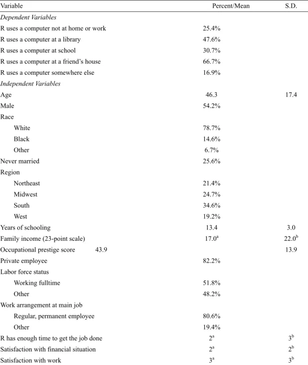
The means, medians, standard deviations, and ranges of the variables are shown in Table 1. As can be seen in the table, overall 25.4% of the respondents used computers not at home or work. Among the subsamples, a friend’s house was the most common place to use a computer other than one’s home or work (66.7%); library was the second most popular location to do so (47.6%); 30.7% used computers at school; and only 16.9% used computers somewhere else.

The average age of respondents was 46.3 years with a range from 18 to 89. Males made up 54.2% of the sample. Whites accounted for 78.7% of the sample, African Americans 14.6%, and other races 6.7%. The never married accounted for 25.6%. Of the total responses, 34.6% resided in the South. The average year of schooling was 13.4 years. The median family income was 17, which indicates that the median family income of the respondents was between $35,000 and $39,999. The average occupational prestige score was 43.9. The majority of respondents (82.2%) were private employees. Moreover, 48.2% of the respondents did not work full-time. Of the respondents, 80.6% were permanent employees. At the same time, 45.2% responded that it was very true that they had enough time to get the job done. In total, about 30% were satisfied with their financial situations, and some 28% agreed that satisfaction came from work.

It must be acknowledged that the sample sizes for variables concerning computer use at school, library, friend’s house, and somewhere else are relatively small, but they are adequate to generate reliable estimates.

Computer Use Not at Home or Work

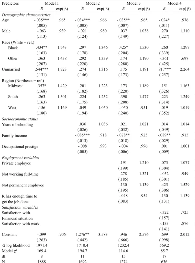
Table 2 reports the estimates of four nested logistic regression models predicting computer use not at home or work. The demographic variables are the predictors in the first model. In Model 2, the model χ2 increases

by 25.3 (=194.7–169.4), which is extremely statistically significant at beyond the 0.001 level with a difference of 3 degrees of freedom. This suggests that socio-economic status is very important in predicting computer use at locations other than home or work. The employment variables are added to Model 3, but the model χ2 _decreases _{by 80.1 because of the}

significant loss of cases. The satisfaction variables added to Model 4 reduce the model χ2 _{by 28.9 also due}

to the loss of many cases. Model 2 is the best-fitting model, on which the interpretations mainly focus.

As shown in Model 2, age has a highly significant negative effect on the dependent variable. This result is consistent with our expectation. The older the respondents are, the less likely they are to use computers outside home or work. For each additional year increase in age, the probability of using computers not at home or work would decrease by 3.4%. Age has a consistent effect on the dependent variable across the four models.

Family income consistently shows a significant effect on the dependent variable in Models 2, 3, and 4. In Model 2, there is a highly significant negative relationship between family income and computer use not at home or work. For each additional level increase in family income, the probability of using computers not at home or work will decrease about 8%. This coincides with our hypothesis. The dummy variable for the unmarried is marginally significant at the 0.06 level. However, other variables in Model 2 do not have a significant effect on computer use outside home or work at the 0.05 level.

In Model 4, the relationship between satisfaction with financial situation and computer use outside home or work is negative and significant. Each additional level increase in satisfaction with financial situation would decrease the likelihood of using computers at locations other than home or work by about 27%. This result supports the hypothesis that those who are satisfied with financial situations are less likely to use computers outside home or work.

(6)

Computer Use in Library

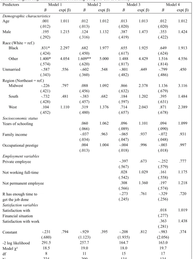
Table 3 shows the results of logistic regression estimates predicting the use of computers in a library other than at home or work. Among the four models, only the model χ2 _{in Model 1 is statistically significant}

at the 0.05 level, indicating that this is the best-fitting model. It is evident from Model 1 that there exist significant differences in the use of computers in libraries. Compared with whites, African Americans and other races are more likely to use computers in a library. This finding is consistent with our expectation. Socioeconomic status, employment status, satisfaction variables, and other demographic variables do not influence computer use in libraries. These results suggest that people are likely to use computers at libraries regardless of their backgrounds except for racial differences.

Computer Use at School

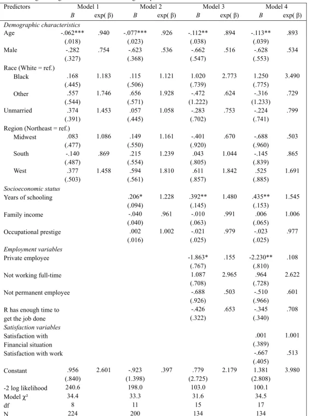
The results of logistic regression analysis predicting computer use at school other than at home or work are reported in Table 4. Compared with the third model, the model χ2 _{in Model 4 increases by 2.9, which is very}

significant at the 0.01 level. Model 4 is the best fitting model. The interpretations are focused on Model 4.

The results in Model 4 show that there is very significant and negative relationship between age and computer use at school other than home or work. The older the respondents are, the less likely they are to use computers at school. For each additional year in age, the probability of computer use at school would decrease by roughly 11%. The effect of age is quite consistent across the four models. The relationship between education and computer use at school is significant and positive, suggesting that the more educated respondents are, the more likely they are to use computers at school. This result runs counter to our hypothesis. Perhaps, computer ownership is less important here. Education familiarizes people to school and therefore facilitates the use of computers at

school. Unexpectedly, private employees are significantly less likely to use computers at school than government employees, probably because they normally do not need to. The other variables have no significant impact on the respondents’ computer use at school.

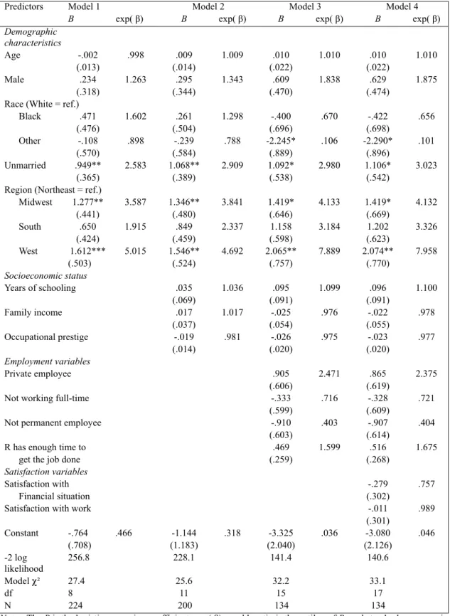
Computer Use at a Friend’s House

Table 5 shows the logistic regression estimates of four nested models predicting computer use at a friend’s house versus at home or work. Model 1 includes only demographic variables. In the second model, the socioeconomic status variables are added as predictors and do not improve the model fit, indicating that these variables do not influence computer use at a friend’s house. Model 3 is a better model than Model 2. The χ2 in the third model increases by 6.6 (=32.2 – 25.6) through adding the employment variables, which is highly significant at the 0.01 level with a difference of 4 degrees of freedom. But, none of the added variables are significant at the 0.05 level. The last model fit is improved by 0.9 by adding two satisfaction variables. The following interpretation is based on Model 4.

The two demographic variables--marital status and region--have a consistent effect on the dependent variable in the four models. As hypothesized, the unmarried are more likely to use computers at friends’ houses than the married. There are regional differences in using computers at friends’ houses. Compared with respondents in the Northeast, those living in the Midwest and West are more likely to use computers at friends’ houses as expected, but those residing in the South do not differ significantly from those in the Northeast. Other race is about 90% less likely than whites to use computers at friends’ houses, but there is no significant difference between blacks and whites in this regard. Age and gender have no effect on respondents’ computer use at friends’ houses, nor does socioeconomic status. The variable having enough time to get the job done is marginally significant at the

(7)

0.06 level. However, other variables have no significant effect on computer use at a friend’s house.

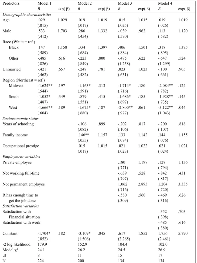
Computer Use Somewhere Else

As shown in Table 6, logistic regression estimates for determinants of using computers somewhere else indicate that the model χ2’sin the first two models are statistically significant at the 0.01 level whereas the model χ2’s in Models 3 and 4 are not significant. The model χ2 _{in Model 2}_{increases by 2.1, which is very}

significant at the 0.01 level with a difference of 3 degrees of freedom. The interpretations below are mainly based on Model 2, the best fitting model.

In Model 2, region is a significant predictor. Unexpectedly, the respondents in the Midwest and West are much less likely than those in the Northeast to use computers somewhere else outside home or work. However, Southerners are not much different from those in the Northeast in using computers somewhere else. Other demographic variables make no significant difference.

There is a very significant and positive relationship between family income and computer use somewhere else, counter to our hypothesis. This result might reflect the possibility that people with higher income are more likely to have laptop computers and use them during travel or leisure activities. The other variables do not significantly impact the respondents’ computer use somewhere else.

Conclusion

One of the findings of this study is that about a quarter of American adults used computers outside home or workplace. Among those who did use computers outside home or work, close to half of them used computers in libraries, two thirds used computers at friends’ houses, nearly one third used them at schools, and 17% used them in other locations.

The main finding is that demographic variables (e.g., age, race, marital status, and region), socio-economic

status (e.g., education, family income), self employment, and satisfaction with financial situation play significant roles in predicting computer use at locations other than home or work. This suggests that many factors impact people’s location choice of computer use outside home or work. Specifically, the older are less likely than the younger to use computers outside home or work. African Americans and other racial minorities are more likely than whites to use computers in libraries. The more educated the respondents are, the more likely they are to use computers at school. Private employees are less likely than their counterparts to utilize computers at school. Other racial minorities are less likely than whites to use computers at friends’ houses. The unmarried are more likely than the married to utilize computers at friends’ houses, and respondents in the Midwest and West are also more likely to do so than those in the Northeast. Respondents in the Midwest and West are less likely than those in the Northeast to use computers somewhere else other than at home or work, and lower income people are also less likely to do so than their higher income counterparts. Occupation and gender make no difference.

The finding that so many people use computers in libraries suggests that libraries attract many people and can facilitate the use of updated computers and applications. In order for libraries to attract users, advanced information technologies must be frequently updated. The fact that certain groups are more or less likely to use computer outside home or work implies that there exist gaps in computer ownership and usage. It is indispensable for institutions to provide more computer infrastructure support and services for customers in public places. This is especially important in serving people who are economically and technologically disadvantaged.

Besides the factors explored in this study, other variables such as computer literacy, computer ownership, and Internet skills could influence the

(8)

location choice of computer use. When available, these predictors should be included in analysis. Future research should also try to increase sample sizes in analyzing the patterns of specific location choices of computer use such as in a library and at a friend’s house. Consideration may be given to other locations of computer usage such as on airplanes, on trains or subways, and in hotels. Our knowledge about location choice patterns of computer use will be more complete and accurate with these additions.

References

Betty, J. Y. (2000). Gender differences in student attitudes toward computers. Journal of Research on

Computing in Education, 33(2), 204-216.

Borja, R. R. (2003). Children’s home computer use linked to learning and weight. Education Week,

23(10), 14.

Calvert, S. L., Rideout, V. J., Woolard, J. L., Barr, R. F., & Strouse, G. A. (2005). Age, ethnicity, and socioeconomic patterns in early computer use.

American Behavioral Scientist, 48(5), 590-607.

Chu, A., Huber, J., Mastel-Smith, B., & Cesario, S. (2009). Partnering with seniors for better health: Computer use and Internet health information retrieval among older adults in a low socioeconomic community. Journal of the Medical Library

Association, 97(1), 11-19.

Colley, A., & Comber, C. (2003). Age and gender differences in computer use and attitudes among secondary school students: What has changed?

Educational Research, 45(2), 155-165.

Davis, J., & Smith, T. W. (2005). General social

surveys, 1972-2004 [machine-readable file].

Chicago, IL: National Opinion Research Center. DeBell, M., & Chapman, C. (2003). Computer and

Internet use by children and adolescents in 2001: Statistical analysis report. Washington, DC: U. S.

Department of Education, National Center for Education Statistics.

Frazel, M. (2007). Tech for tinies: How young is too young to use computers? Library Media Connection,

25(3), 56-58.

Gerber, E. (2003). The benefits of and barriers to computer use for individuals who are visually impaired. Journal of Visual Impairment & Blindness,

97(9), 536-551.

Gietzelt, D. (2001). Computer and Internet use among a group of Sydney seniors: A pilot study. Australian

Academic & Research Libraries, 32(2), 137-152.

Green, F., Felstead, A., Gallie, D., & Zhou, Y. (2007). Computers and pay. National Institute Economic

Review, 201, 63-75.

Gross, M., Dresang, E. T., & Holt, L. E. (2004). Children’s in-library use of computers in an urban public library. Library & Information Science

Research, 26(3), 311-337.

Hinchliff, G. (2008). Toddling toward technology: Computer use by very young children. Children and

Libraries, 6(3), 47-49.

Huang, G. G.., & Du, J. (2002). Computer use at home and at school: Does it relate to academic performance? Journal of Women and Minorities in

Science and Engineering, 8(2), 201-217.

Hunley, S. A., Evans, J. H., Delgado-Hachey, M., Krise, J., Rich, T., & Schell, C. (2005). Adolescent computer use and academic achievement.

Adolescence, 40(158), 307-318.

Kominski, R., & Newburger, E. (1999). Access denied: Changes in computer ownership and use: 1984-1997. Paper delivered at the annual meeting of the American Sociological Association, Chicago, Illinois.

Lauman, D. J. (2000). Student home computer use: A review of the literature. Journal of Research on

Computing in Education, 33(2), 196-203.

Li, X., Atkins., M. S., & Stanton, B. (2006). Effects of home and school computer use on school readiness and cognitive development among head start children: A randomized controlled pilot trial.

(9)

Mann, W. C., Belchior, P., Tomita, M. R., & Kemp, B. J. (2005). Computer use by middle-aged and older adults with disabilities . Technology and Disability,

17, 1-9.

Mitra, A., Steffensmeier, T., Lenzmeier, S., & Massoni, Angela. (1999). Changes in attitudes toward computers and use of computers by university faculty. Journal of Research on Computing in

Education, 32(1), 189-202.

Mitra, A., & Steffensmeier, T. (2000). Changes in student attitudes and student computer use in a computer-enriched environment. Journal of

Research on Computing in Education, 32(3),

417-433.

Namazi, K. H., & McClintic, M. (2003). Computer use among elderly persons in long-term care facilities.

Educational Gerontology, 29(6), 535-550.

Newburger, E. C. (1999). Computer use in the United

States: Population characteristics. Washington, DC:

U.S. Census Bureau.

Newburger, E. C. (2001). Home computers and

Internet use in the United States: August 2000.

Washington, DC: U.S. Census Bureau.

Ono, H., & Tsai, H. J. (2008). Race, parental socioeconomic status, and computer use time outside of school among young American children,

1997 to 2003. Journal of Family Issues, 29(12), 1650-1672.

Peterson, N. B., Dwyer, K. A., & Mulvaney, S. A. (2009). Computer and Internet use in a community health clinic population. Medical Decision Making,

29, 202-206.

Saunders, E. J. (2004). Maximizing computer use among the elderly in rural senior centers.

Educational Gerontology, 30, 573-585.

Schmitz, K. H., Harnack, L., Fulton, J. E., Jacobs, D. R., Gao, S., Lytle, L. A., & Coevering, P. V. (2004). Reliability and validity of a brief questionnaire to assess television viewing and computer use by middle school children. Journal of School health,

74(9), 370-376.

Solvberg, A. M. (2002). Gender differences in computer-related control beliefs and home computer use. Scandinavian Journal of Educational Research,

46(4), 409-426.

Spooner, T. (2003). Internet use by region in the

United States. Washington, DC: Pew Internet &

American Life Project.

Wentworth, N., & Earle, R. (2003). Trends in computer uses as reported in Computers in the

(10)

Table 1. Descriptive Statistics of Variables Used in the Analysis, U.S. Adults

Variable Percent/Mean S.D.

Dependent Variables

R uses a computer not at home or work 25.4% R uses a computer at a library 47.6%

R uses a computer at school 30.7%

R uses a computer at a friend’s house 66.7% R uses a computer somewhere else 16.9%

Independent Variables Age 46.3 17.4 Male 54.2% Race White 78.7% Black 14.6% Other 6.7% Never married 25.6% Region Northeast 21.4% Midwest 24.7% South 34.6% West 19.2% Years of schooling 13.4 3.0

Family income (23-point scale) 17.0a_22.0b

Occupational prestige score 43.9 13.9

Private employee 82.2%

Labor force status

Working fulltime 51.8%

Other 48.2%

Work arrangement at main job

Regular, permanent employee 80.6%

Other 19.4%

R has enough time to get the job done 2a ₃b

Satisfaction with financial situation 2a ₂b

Satisfaction with work 3a ₃b

ª Median.

(11)

Table 2. Logistic Regression Estimates Predicting Computer Use outside Home or work

Predictors Model 1 Model 2 Model 3 Model 4

B exp( β) B exp( β) B exp( β) B exp( β)

Demographic characteristics

Age -.035*** .965 -.034*** .966 -.035** .965 -.024* .976

(.005) (.005) (.007) (.011)

Male -.063 .939 -.021 .980 .037 1.038 .270 1.310

(.113) (.124) (.149) (.227)

Race (White = ref.)

Black .434** 1.543 .297 1.346 .425* 1.530 .260 1.297 (.163) (.178) (.204) (.339) Other .363 1.438 .292 1.339 .174 1.190 -.361 .697 (.207) (.220) (.280) (.425) Unmarried .544*** 1.723 .274 1.316 .175 1.191 .817*** 2.264 (.131) (.146) (.173) (.257)

Region (Northeast = ref.)

Midwest .357* 1.429 .201 1.223 .173 1.189 .151 1.163 (.168) (.182) (.220) (.326) South .263 1.301 .224 1.252 .390 1.477 .223 1.249 (.163) (.175) (.208) (.314) West .156 1.169 .049 1.050 -.050 .951 .019 1.019 (.180) (.194) (.240) (.352) Socioeconomic status Years of schooling .036 1.036 .021 1.021 .014 1.014 (.026) (.032) (.049) Family income -.085*** .918 -.078** .925 -.089** .915 (.013) (.018) (.029) Occupational prestige -.008 .993 -.004 .996 .001 1.001 (.005) (.006) (.009) Employment variables Private employee .191 1.210 .075 1.077 (.199) (.304)

Not working full-time .278 1.321 -.052 .949

(.185) (.301)

Not permanent employee .130 1.139 .425 1.529

(.195) (.306)

R has enough time to -.048 .954 .130 1.139

get the job done (.083) (.131)

Satisfaction variables

Satisfaction with -.322 .725

Financial situation (.157)

Satisfaction with work -.133 .876

(.141) Constant -.099 .906 1.276** 3.583 .946 2.576 .699 2.012 (.263) (.442) (.666) (.998) -2 log likelihood 1971.4 1710.4 1232.4 569.2 Model χ² 169.4 194.7 114.6 85.7 df 8 11 15 17 N 1888 1692 1274 636

Notes: The B is the logistic regression coefficient; exp( β) or odds ratio is the antilog of B; and standard errors are

in parentheses.

(12)

Table 3. Logistic Regression Estimates Predicting Computer Use in a Library

Age .001 1.011 .012 1.012 .013 1.013 .012 1.012

(.012) (.013) (.020) (.020)

Male .195 1.215 .124 1.132 .387 1.473 .353 1.424

(.292) (.316) (.419) (.422)

Race (White = ref.)

Black .831* 2.297 .682 1.977 .655 1.925 .649 1.913 (.424) (.450) (.617) (.624) Other 1.400* 4.054 1.609** 5.000 1.488 4.429 1.516 4.556 (.574) (.620) (.817) (.814) Unmarried -.587 .556 -.602 .548 -.801 .449 -.799 .450 (.343) (.360) (.482) (.486)

Midwest -.226 .797 .088 1.092 .866 2.378 1.136 3.116 (.421) (.456) (.632) (.679) South -.732 .481 -.383 .682 .184 1.202 .395 1.484 (.428) (.457) (.597) (.631) West .104 1.110 .319 1.376 .714 2.043 .871 2.389 (.452) (.480) (.657) (.678) Socioeconomic status Years of schooling .060 1.062 .096 1.101 .094 1.099 (.066) (.089) (.090) Family income -.037 .963 -.065 .937 -.072 .931 (.034) (.047) (.048) Occupational prestige .004 1.004 -.004 .996 -.003 .997 (.013) (.018) (.018) Employment variables Private employee -.397 .673 -..252 .777 (.567) (.579)

Not working full-time .028 1.029 .161 1.175

(.542) (.558)

Not permanent employee .308 1.360 .197 1.218

(.566) (.574)

R has enough time to -.273 .761 -.329 .720

Satisfaction with .018 1.019

Satisfaction with work .363 1.438

(.281) Constant -.231 .794 -.929 .395 -.208 .812 -.983 .374 (.680) (1.123) (1.935) (2.056) -2 log likelihood 291.5 257.7 164.7 163.0 Model _χ² 18.5 19.0 18.0 19.7 df 8 11 15 17 N 224 200 134 134

in parentheses.

(13)

Table 4. Logistic Regression Estimates Predicting Computer Use at School

Age -.062*** .940 -.077*** .926 -.112** .894 -.113** .893

(.018) (.023) (.038) (.039)

Male -.282 .754 -.623 .536 -.662 .516 -.628 .534

(.327) (.368) (.547) (.553)

Race (White = ref.)

Black .168 1.183 .115 1.121 1.020 2.773 1.250 3.490 (.445) (.506) (.739) (.775) Other .557 1.746 .656 1.928 -.472 .624 -.316 .729 (.544) (.571) (1.222) (1.233) Unmarried .374 1.453 .057 1.058 -.283 .753 -.224 .799 (.391) (.445) (.702) (.741)

Midwest .083 1.086 .149 1.161 -.401 .670 -.688 .503 (.477) (.550) (.920) (.960) South -.140 .869 .215 1.239 .043 1.044 -.145 .865 (.487) (.554) (.805) (.839) West .377 1.458 .594 1.810 .611 1.842 .525 1.691 (.503) (.561) (.857) (.885) Socioeconomic status Years of schooling .206* 1.228 .392** 1.480 .435** 1.545 (.094) (.145) (.153) Family income -.040 .961 -.010 .991 .006 1.006 (.040) (.063) (.065) Occupational prestige .002 1.002 -.021 .979 -.023 .977 (.016) (.025) (.025) Employment variables Private employee -1.863* .155 -2.230** .108 (.767) (.810)

Not working full-time 1.087 2.965 .964 2.622

(.708) (.728)

Not permanent employee -.688 .503 -.510 .601

(.926) (.966)

Satisfaction with .001 1.001

(.405) Constant .956 2.601 -.923 .397 .779 2.179 1.381 3.980 (.840) (1.398) (2.725) (2.808) -2 log likelihood 240.6 198.0 103.0 100.1 Model χ² 34.4 33.3 31.6 34.5 df 8 11 15 17 N 224 200 134 134

in parentheses.

(14)

Table 5. Logistic Regression Estimates Predicting Computer Use at a Friend's House

Demographic characteristics Age -.002 .998 .009 1.009 .010 1.010 .010 1.010 (.013) (.014) (.022) (.022) Male .234 1.263 .295 1.343 .609 1.838 .629 1.875 (.318) (.344) (.470) (.474)

Race (White = ref.)

Black .471 1.602 .261 1.298 -.400 .670 -.422 .656 (.476) (.504) (.696) (.698) Other -.108 .898 -.239 .788 -2.245* .106 -2.290* .101 (.570) (.584) (.889) (.896) Unmarried .949** 2.583 1.068** 2.909 1.092* 2.980 1.106* 3.023 (.365) (.389) (.538) (.542)

Midwest 1.277** 3.587 1.346** 3.841 1.419* 4.133 1.419* 4.132 (.441) (.480) (.646) (.669) South .650 1.915 .849 2.337 1.158 3.184 1.202 3.326 (.424) (.459) (.598) (.623) West 1.612*** 5.015 1.546** 4.692 2.065** 7.889 2.074** 7.958 (.503) (.524) (.757) (.770) Socioeconomic status Years of schooling .035 1.036 .095 1.099 .096 1.100 (.069) (.091) (.091) Family income .017 1.017 -.025 .976 -.022 .978 (.037) (.054) (.055) Occupational prestige -.019 .981 -.026 .975 -.023 .977 (.014) (.020) (.020) Employment variables Private employee .905 2.471 .865 2.375 (.606) (.619)

Not working full-time -.333 .716 -.328 .721

(.599) (.609)

Not permanent employee -.910 .403 -.907 .404

(.603) (.614)

R has enough time to .469 1.599 .516 1.675

(.301) Constant -.764 .466 -1.144 .318 -3.325 .036 -3.080 .046 (.708) (1.183) (2.040) (2.126) -2 log likelihood 256.8 228.1 141.4 140.6 Model χ² 27.4 25.6 32.2 33.1 df 8 11 15 17 N 224 200 134 134

Notes: The B is the logistic regression coefficient; exp( β) or odds ratio is the antilog of B; and standard errors are in

parentheses.

(15)

Table 6. Logistic Regression Estimates Predicting Computer Use Somewhere Else

B exp( β) B exp( β) B exp( β) B exp( β)

Age .029 1.029 .019 1.019 .015 1.015 .019 1.019

(.015) (.017) (.025) (.026)

Male .533 1.703 .286 1.332 -.039 .962 .113 1.120

(.412) (.454) (.570) (.582)

Race (White = ref.)

Black .147 1.158 .334 1.397 .406 1.501 .318 1.375 (.589) (.684) (.884) (.895) Other -.485 .616 -.223 .800 -.475 .622 -.647 .524 (.826) (.849) (1.258) (1.299) Unmarried -.421 .657 -.248 .781 .023 1.023 -.100 .905 (.462) (.482) (.631) (.661)

Midwest -1.624** .197 -1.163* .313 -1.714* .180 -2.084** .124 (.544) (.591) (.716) (.782) South -1.052* .349 -.879 .415 -1.686* .185 -1.928** .145 (.487) (.551) (.697) (.735) West -1.666** .189 -1.675* .187 -2.800** .061 -3.122** .044 (.604) (.680) (.977) (1.043) Socioeconomic status Years of schooling -.106 .899 -.202 .817 -.200 .818 (.082) (.106) (.107) Family income .146** 1.157 .133 1.142 .144 1.155 (.055) (.074) (.076) Occupational prestige .015 1.015 .021 1.022 .021 1.021 (.017) (.023) (.024) Employment variables Private employee .180 1.197 .128 1.136 (.771) (.794)

Not working full-time -.639 .528 -.842 .431

(.797) (.817)

Not permanent employee 1.062 2.893 1.204 3.335

(.716) (.720)

(.380) Constant -1.704* .182 -3.109* .045 .617 1.852 1.756 5.790 (.852) (1.506) (2.265) (2.461) -2 log likelihood 179.9 152.9 104.4 102.0 Model χ² 24.1 26.2 24.5 26.9 df 8 11 15 17 N 224 200 134 134

in parentheses.