Semantic Matching and Annotation of Images by Self-Organizing Maps

(1)

Computing, Information and Control ICIC International c°2008 ISSN 1349-4198

Volume x, Number 0x, x 2008 pp. 0–0

SEMANTIC MATCHING AND ANNOTATION OF IMAGES BY SELF-ORGANIZING MAPS

Hsin-Chang Yang

Department of Information Management National University of Kaohsiung

Kaohsiung, 811, Taiwan [email protected] Chung-Hong Lee Department of Electrical Engineering National Kaohsiung University of Applied Sciences

Kaohsiung, Taiwan [email protected]

Abstract. Image retrieval has attracted lots of attention from both researchers and

practitioners. Different methodologies as well as commercial systems have been proposed and developed to tackle this task. Most of these systems are based on one or both of two major image retrieval schemes, namely annotation-based image retrieval and content-based image retrieval. The former is simple and accurate, provided some annotations have been added to the images. However, such annotations are often missed in most of images available in large datasets such as the WWW. To tackle this deficiency, we propose a method that could automatically annotating images with some keywords that could feasibly describe the semantics of the images. A set of training images as well as their annotations are trained to find the relationships between images as well as between keywords. New image could then be annotated and retrieved according to such relation-ships. Our preliminary experiments suggest promising result in both image annotation task and image retrieval task.

Keywords: Image Annotation, Image Retrieval, Self-Organizing Map

1. Introduction. Recently the task of image retrieval has received a great deal of at-tention from the web community since there are so many useful images on web pages. In fact, image retrieval has been studied for decades in library science and computer sci-ence communities. Image retrieval is a branch of information retrieval whose task is to retrieve some pieces of information (the documents) to meet a user’s information needs according to certain (semantic) relevance measurements. Currently most information re-trieval systems retrieve documents based on their ’contents’. That is, they measure the relevance between the query and a document according to internal representations or de-rived features. Such representations or features will vary for different document styles and retrieval schemes. For text retrieval systems, the contents are often represented by a set of selected keywords that are intended to capture the semantics of the documents. Many studies have successfully represented the semantics of text documents (Baeza-Yates & Ribeiro-Neto 1999). For image retrieval systems, the representation of image content generally fall into two types. The first is to represent an image with a set of keywords

(2)

2 H. C. YANG AND C. H. LEE

that could describe the content of the image. Such keywords are used as annotations for an image and thus we may call this type of representation scheme the annotation-based image representation and call the task of retrieval by annotation the annotation-based im-age retrieval. The other representation contains a set of visual features extracted from the image that hopefully may effectively represent the image. We call this type the content-based image representation and the task of retrieval by content the content-content-based image retrieval. Many schemes have been proposed to describe the image contents for content-based image representation (De Marsicoi, Cinque & Levialdi 1997, Doermann 1998, Gupta & Jain 1997). However, the correct interpretation of image content is always difficult and imprecise. And users are forced to express their needs by means of visual features, which are difficult for common users. On the other hand, annotation-based image retrieval has the advantages of simplicity and accuracy. For simplicity we mean that a user could easily represent his need in simple keywords. In the mean time, the matching of the user query and image content (by means of annotations) is also well studied and could be accurately made. From the user’s perspective, annotation-based image retrieval is much easier and instinctive. However, such advantages rely on correct annotations of images, which are often absent for images in large databases.

To meet the requirement of annotation-based image retrieval, images should be an-notated. Early image databases often annotated images manually. Manual annotations are generally considered correct. However, a lot of time must be wasted in the annota-tion process. Thus manual annotaannota-tion is not applicable to large datasets. For datasets that are sufficiently large, e.g. the WWW, automatic annotation is necessary to perform annotation-based image retrieval. In this work, we propose a method that can automat-ically annotate the images with thematic keywords. The annotation process begins with a clustering process that groups similar image segments into clusters. The annotations of these image segments are also clustered. We adopt the self-organizing map model to cluster images as well as annotations. After the clustering process, we establish the re-lationships between image clusters and annotation clusters through a labeling process. Basically, this process is similar to a multilingual text mining process that discovers rela-tionships between two languages. The image segments could resemble to a set of symbolic terms, which are then matched to the other set of terms that come from the annotations. Therefore, the major contribution of our work is to use a proposed multilingual text min-ing process to establish the relationships between images and annotations, which in turn achieve the automatic image annotation tasks.

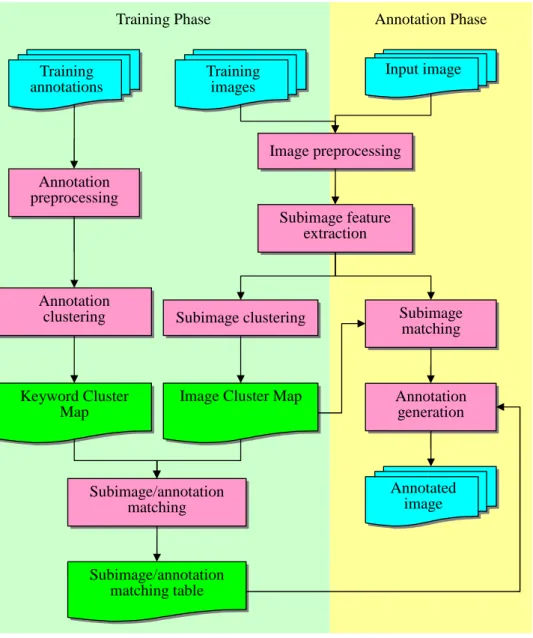
Fig. 1 depicts an overview of the proposed method. In the training phase, both images and their annotations are preprocessed to obtain suitable feature representations. These features are then clustered into subimage clusters and annotation clusters respectively. Each subimage cluster consists of potentially similar image segmentations. On the other hand, an annotation cluster contains a set of keywords that are closely related. A match-ing process is applied to match the subimages and annotation keywords and create the relationships between them, which are stored in the subimage/annotation matching table (SAMT). When an input image comes, it is also preprocessed into a set of subimages. Each subimage is then annotated with the help of SAMT and integrated into the final annotation of the input image.

We address some words about the motivation and advantages of this work. The mo-tivation of this work is to propose an automatic technique that will alleviate the need

(3)

Subimage feature extraction Training images Input image Subimage clustering Subimage/annotation matching Subimage matching Annotation generation Subimage/annotation matching table

Image Cluster Map Training annotations Annotation clustering Image preprocessing Keyword Cluster Map

Training Phase Annotation Phase

Annotated image Annotation

preprocessing

Figure 1. The processing stages and functional components of the pro-poses method.

of human intervention on annotating images. The major advantages of this method are three-fold. First, our method is full automatic that requires no manual processing. This will allow our method being applicable on large scale datasets such as the World Wide Web. Second, we use a discovery algorithm that resembles a text mining scheme which could find implicit associations between images and keywords. This scheme requires no sophisticated image feature representations which are difficult to define. Finally, out method could be extended to other tasks, such as multilingual text mining, that require the discovery of associations between two sets of symbols. Such tasks are always difficult and our method may provide a plausible solution to them.

2. Related Work. Recently, a number of models have been proposed for image annota-tion. One of the first attempts at image annotation was reported by Mori, Takahashi &

(4)

Oka (1999), who tiled images into grids of rectangular regions and applied a co-occurrence model to words and low-level features of such tiled image regions. Duygulu, Barnard, de Freitas & Forsyth (2002) described images using a vocabulary of blobs. First, regions are created using a segmentation algorithm like normalized cuts. For each region, fea-tures are computed and then blobs are generated by clustering the image feafea-tures for these regions across images. Each image is generated by using a certain number of these blobs. Their Translation Model applies one of the classical statistical machine translation models to translate from the set of blobs forming an image to the set of keywords of an image. Correlation LDA proposed by Blei & Jordan (2003) extends the Latent Dirichlet Allocation (LDA) Model (Blei, Ng & Jordan 2003) to words and images. This model assumes that a Dirichlet distribution can be used to generate a mixture of latent factors. This mixture of latent factors is then used to generate words and regions. Expectation-Maximization is used to estimate this model. Barnard, Duygulu, de Freitas, Forsyth, Blei & Jordan (2003) proposed and tested various statistical models to learn the joint probabilities of image regions and words. Li & Wang (2003) proposed a two-dimensional multiresolution hidden Markov models to relate images and concepts. Jeon, Lavrenko & Manmatha (2003) assumed that image annotation could be viewed as analogous to the cross-lingual retrieval problem and proposed the cross-media relevance model for this problem. They used the same discrete features as in (Duygulu et al. 2002) and showed that a considerable improvement in performance was attained. A continuous relevance model was proposed in (Lavrenko, Manmatha & Jeon 2004) to use continuous features with significant improvement in performance. Given the problems with variable length annotations, Feng, Manmatha & Lavrenko (2004) proposed a Bernoulli model to improve annotation performance while in (Lavrenko, Feng & Manmatha 2004), the authors pro-posed the Normalized Continuous Relevance Model to pad the annotations to fixed length and still use a multinomial to achieve the same effect. They showed that the performance of the model on the same dataset was considerably better than the models proposed by Duygulu et al. (2002) and Mori et al. (1999). Metzler & Manmatha (2004) segmented training images, connecting them and their annotations in an inference network, whereby an unseen image is annotated by instantiating the network with its regions and propagat-ing belief through the network to nodes representpropagat-ing the words. Oliva & Torralba (2001) showed that images can be described with basic scene labels such as ‘street’, ‘buildings’ or ‘highways’, using a selection of relevant low-level global filters. They further showed how simple image statistics can be used to infer the presence and absence of objects in the scene (Torralba & Oliva 2003).

3. Image and Annotation Preprocessing and Clustering. In this section we will describe the preprocessing steps that transform the images and annotations into suitable feature representations. We then describe how to cluster images and annotations with self-organizing maps. First a training image I is segmented into a set of subimages Ii, 1 ≤

i ≤ ni, where ni is the number of subimages for I. Two kinds of subimage segmentation methods are adopted. The first is uniform block segmentation that segments images into regular blocks of subimages. This method is simple but may produce subimages without consistent meaning. The other method is to use some semantic regional segmentation schemes such as Blobworld (Carson, Belongie, Greenspan & Malik 2002) and normalized cuts (Shi & Malik 2000) to produce semantically coherent subimages. This kind of method

(5)

has the advantage of producing subimages with coherent semantic meaning. However, further processing of such subimages may be difficult since they may have various shapes and sizes.

For the block segmentation scheme, the image I is segmented into ni fixed-size blocks. There are two choices for the sizes of blocks. The first is to fix the number of blocks, i.e. ni, for each image. The second is to fix the size of blocks, whose sizes could be varied. Our method makes no difference between these choices. However, fixed ni is simpler and could be applied to various sizes of images. Thus we will segment every image into a fixed number of subimages. That is, ni is a fixed number for every image. After segmentation, the color histogram of each subimage Ii for image I is calculated and normalized into a feature vector PIi as follows:

PIi = (bk), 1 ≤ k ≤ K

bk =

c(Ii, k) arg maxkbk

. (1)

In Eq. 1, K is the number of slots in the color histogram and c(Ii, k) is the pixel count of color k in Ii. Thus each subimage Ii is transformed into a fixed-size vector PIi. Similar

encoding method is used in region-based segmentation. An image I is segmented into semantic regions (subimages) Ii using Blobworld algorithm. Note that each image may have different ni for region-based segmentation. Each subimage is then transformed into a vector using Eq. 1.

We now describe the encoding method for the annotations. Each training image is accompanied with a set of annotation keywords. Let AI = {aIj|1 ≤ j ≤ ωI} denote the

set of annotation keywords for image I, where ωIis the number of annotation keywords for

I. We collect all annotation keywords for all training images and obtain the vocabulary V = {vj|1 ≤ j ≤ M}:

V =[

I

AI. (2)

AI is then transformed into a vector WI = (wIj), 1 ≤ j ≤ M as follows:

wIj =

½

1 if aIj ∈ V

0 otherwise (3)

M is the size of vocabulary. We let all subimages of I be annotated with the same set of annotation keywords AI. Thus each subimage Ii of I is also transformed to a keyword vector WIi, such that ∀i, WIi = WI. After the encoding process described in Eq. 1 and

Eq. 3, a subimage Ii is transformed to two vectors simultaneously, namely PIi and WIi.

We concatenate these vectors and obtain the overall feature vector FIi for Ii.

We then perform two clustering processes on all FIi using the self-organizing map

algorithm. The first process clusters concatenated feature vectors FIi and the second

process clusters PIi and WIi individually. The SOM algorithm is described below:

Step 1: Randomly select a training vector xi.

Step 2: Find the neuron j with synaptic weights wj which is closest to xi, i.e.

||xi− wj|| = min

(6)

Step 3: For every neuron l in the neighborhood of neuron j, update its synaptic weights by

wnew

l = woldl + α(t)(xi− woldl ), (5) where α(t) is the training gain at time stamp t.

Step 4: Increase the time stamp t. If t reaches the preset maximum training time T , halt the training process; otherwise decrease α(t) and the neighborhood size, goto Step 1.

The vector xi could be replaced by FIi, PIi, or WIi whenever appropriate. The reason

to perform two different clustering processes is that we wish to discover as much the relationships between images and annotations as possible. The discovery process will be discussed in the next section. Note that the first clustering process generates one feature map and the second process should generate two feature maps.

When the concatenated training vectors FIi are used, the SOM clusters these vectors

according to both visual features and annotation texts. Since we use color histogram to describe the visual properties of images, the size of PIi is generally fixed. On the

other hand, different set of images may produce different set of vocabularies and produce various-sized WIi. When the size of PIi, K, and the size of WIi, M, are considerably

different, the clustering process will reduce to the individual cases, i.e. training with either PIi or WIi. Thus we should balance the contributions come from visual features

and annotation texts when calculating the similarity in Eq. 4. One simple way is to multiply the PIi part by a factor

q M K.

4. Automatic Image Annotation. After the clustering process, a discovery process is then applied to the clustering result to find the associations between subimages and keywords. First we should establish the association between each subimage and one of the neurons using a labeling process, which is described as follows. Each subimage’s feature vector xi is compared to every neuron’s weight vector in the map. We will label the ith subimage to the jth neuron if they satisfy Eq. 4. After the labeling process, each subimage is labeled to some neuron or, from a different point of view, each neuron is labeled by a set of subimages. We record the labeling results and obtain the image cluster map (ICM). In the ICM, each neuron is labeled by a list of subimages which are considered similar and are in the same cluster. ICM could be constructed when the input vectors are PIi.

When the input vectors are WIi, the labeling process will create the keyword cluster map

(KCM), which each neuron represents a cluster of keywords. When the input vectors are FIi, we should label the PIi and WIi parts of FIi separately to obtain ICM and KCM

respectively.

For the case of concatenated training vectors, only a map is generated. After the labeling process, a neuron is labeled with both a set of subimages and keywords. Both relationships between images and between annotation keywords should be discovered from this map. Moreover, the relationships between images and keywords could also be directly derived from this map. However, the clustering result may be incoherent since we combine visual features and annotation keywords together. For example, two subimages that have similar visual features may be annotated differently. Such inconsistency will deteriorate the results of the clustering process as well as the labeling process. The key to use this kind of vectors is the precise segmentation and description of subimages. A subimage is

(7)

annotated with keywords that belong to clusters associated with the same neuron. To annotate an input image I, we first segment it into subimages Ii. Each subimage is then compared to all neurons’ synaptic weight vectors in ICM to find the best match, say neuron j. We should then annotate Ii with those keywords that labeled to neuron j in KCM. The overall annotations for image I is obtained by aggregating all annotations of its subimages as follows:

AI = {aIj|Ii ⊂ I, aIj ∈ AIi, 1 ≤ j ≤ ωI}, (6)

where AIi is the set of annotation keywords of subimage Ii. To obtain better result, we

could count the time of each keyword appeared in all AIi and select only those keywords

that appear over certain times.

For the other case of training PIi and WIi separately, the clustering and labeling

process should work well. Two different maps are trained and labeled to generate KCM and ICM respectively. The relationships between images could be easily discovered from ICM. Meanwhile, the relationships between keywords could be discovered from KCM. This scheme’s difficulty comes from the discovery of relationships between subimages and keywords. We should develop a method to associate clusters in KCM with those in ICM. For a cluster in ICM, we first aggregate the annotation keywords of the subimages in this cluster. Let Cj denote the set of subimages associated with neuron j in the ICM. We aggregate the annotation keywords into a vector cj as follows:

cj = _ Ii∈Cj

WI. (7)

Note that the elements of WI are either 0 or 1 and the ∨ operator performs the bitwise OR operation over all annotation vectors of images in Cj. cj is then compared to all synaptic weight vectors of KCM to find the best match neuron. The association between these two neurons is recorded in the subimage/annotation matching table (SAMT), which is depicted in Fig. 1. Note that different image clusters may match the same keyword clusters. When SAMT is constructed, an input image I is first segmented into a set of subimages Ii. Each subimage is then labeled to some neuron in ICM. The annotations for this subimage could be selected using SAMT. The same method described in Eq. 6 could be used to obtain the overall annotations for the entire image.

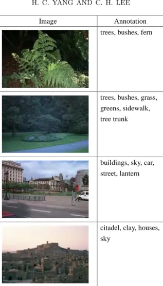
5. Experiment Result. We performed the experiments on the Groundtruth database of Washington University (Washington 1999). Some example images along with their annotations are depicted in Fig. 2. Two corpora of images were constructed. Corpus 1 and Corpus 2 contain 1000 and 100 images that randomly selected from the database respectively. All images are accompanied with annotations. Both corpora are divided into train set and test set, which contains 70% and 30% of images respectively. Table 1 lists some statistics of the used corpora. The images in the training set were preprocessed and encoded into feature vectors as described in Sec. 3. In the experiments, we used block segmentation and region-based segmentation to segment images. For block segmentation, each image is segmented into 3 subimages. We adopt Blobworld algorithm for region-based segmentation. We then calculated the color histogram for each subimage. The slot number of the histogram is 512 in the experiments. We normalized the sizes of images to 192 × 128 pixels before the segmentation. The color histogram of a subimage is then

(8)

Image Annotation

trees, bushes, fern

trees, bushes, grass, greens, sidewalk, tree trunk

buildings, sky, car, street, lantern

citadel, clay, houses, sky

Figure 2. Some example images and their annotations from the Groundtruth database

Table 1. Some statistics of the corpora in the experiments. Corpus 1 Corpus 2

Number of images 1000 100 Average number of

keywords per image 6.53 5.72

Vocabulary size 213 118

encoded into a 512-element vector. Its annotation is also transformed into a vector, which length is 213 and 118 for Corpus 1 and Corpus 2 respectively. Table 2 lists some statistics of the segmentation result.

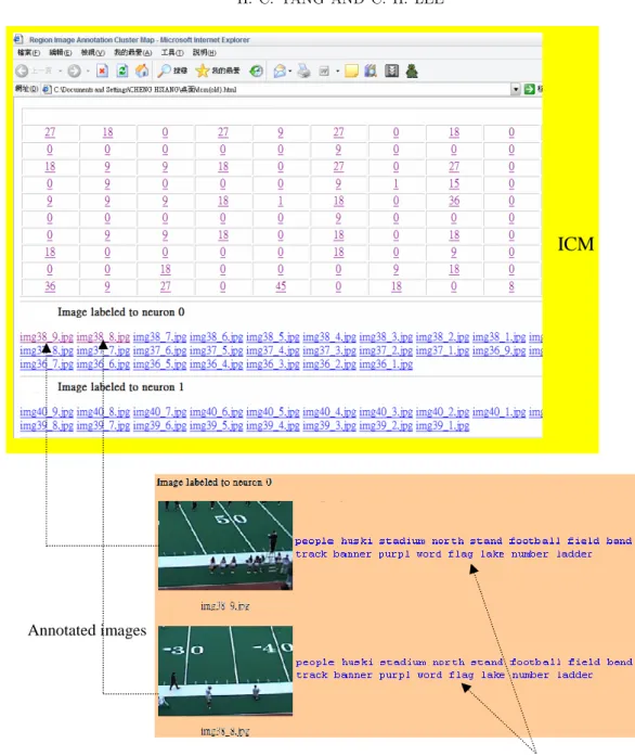
After the preprocessing, we clustered the subimages as described in Sec. 3. The sizes of the self-organizing maps are 20 × 20 and 10 × 10 for Corpus 1 and Corpus 2 respectively. The labeling process is then applied to the clustering result to obtain ICM and KCM. Fig. 3 shows the ICM and KCM of Corpus 2 when the block segmentation and concatenated vector schemes are used. Each grid of the ICM contains a number which is the number of images labeled to the corresponding neuron. The set of images labeled to a neuron

(9)

Table 2. Some statistics of the segmentation result in the experiments. Corpus 1 Corpus 2 Block segmenta-tion Region-based segmentation Block segmenta-tion Region-based segmentation Average number of

subimages Ii per im-age

9 7.3 9 7.1

Size of PIi 512 512 512 512

Size of WIi 213 213 118 118

could be found by clicking on the number. For example, when click on the upper-leftmost neuron, it will show the filenames of the 27 images labeled to this neuron, which is neuron 0. An image can then be retrieved by clicking on its filename. Two images, namely image38 9.jpg and image38 8.jpg, are shown in this figure. The KCM is simply a list of keywords that labeled to all neurons, which is shown in the bottom of the figure. Each line contains the set of keywords that labeled to a neuron. The number in the beginning of each line shows the number of keywords labeled to the corresponding neuron. For example, the first line contains all 19 keywords labeled to neuron 0. After generating these two maps, the annotations of an image could be obtained. Two examples are also shown in Fig. 3. As shown in the figure, the annotations are generated from the ICM and KCM. Since these two images are labeled to the same neuron, they were annotated with the same set of keywords. It is clear that the example shows a positive result of the annotation process.

To evaluate our work, we used the test set of each corpus as input and tried to obtain their annotations. For a test image T , we first segment it into a set of subimages Ti. Each Ti is then labeled to a neuron, say j, in the ICM. The annotations associated with neuron j in WCM are annotated to Ti. The overall annotations of T are aggregated from all annotations of its subimages. We evaluate the result by measuring the performance when we apply these generated annotations to the image retrieval task. A set of keyword queries were sent to the image database that contains the annotated test images. We then measured the performance with the common F -measure (Baeza-Yates & Ribeiro-Neto 1999) which is defined as:

recallq = X(q) ∩ Y (q) X(q) precisionq = X(q) ∩ Y (q) Y (q) Fq = 2 × recallq× precisionq recallq+ precisionq , (8)

where X(q) is the set of correct images to query q and Y (q) is the set of retrieved images to query q. In our experiments, q contains a set of keywords. X(q) and Y (q) are the sets of test images that contain all keywords of q in their original and generated annota-tions respectively. Totally 100 queries were used in our experiments. We tried the four combinations of the segmentation schemes and training vector encoding schemes in our

(10)

ICM

Annotations labeled to neuron 0

KCM

Annotated images

(11)

Table 3. The result of F -measure in the experiments. The terms ’Block’ and ’Region’ stand for block segmentation scheme and region-based segmen-tation were used respectively. The terms ’Concatenated’ and ’Separated’ stand for concatenated vectors and separated vectors were used respectively.

Corpus 1 Corpus 2 Block/Concatenated 0.73 0.66 Block/Separated 0.69 0.75 Region/Concatenated 0.82 0.71 Region/Separated 0.77 0.76

Table 4. The average Hamming distance between correct annotation and generated annotation. Corpus 1 Corpus 2 Block/Concatenated 2.35(0.36) 2.21(0.39) Block/Separated 1.70(0.26) 2.11(0.37) Region/Concatenated 1.27(0.19) 1.93(0.34) Region/Separated 1.18(0.18) 1.67(0.29)

experiments. The result is shown in Table 3. It is clear that our method could produce acceptable result.

Another evaluation scheme is to measure the degree of overlap between the correct annotation and the generated annotation. Since we adopt binary vectors to represent images, the degree of overlap could be measured by the Hamming distance between the annotation vectors in the form of Eq. 3. We calculate the average Hamming distance among all training images as follows:

H = 1 N X 1≤i≤N 1 M X 1≤j≤M |wI_ij − aI_ij|, (9)

where wI_ij is the jth component of the vector for training image Ii and aI_ij is the jth component of the generated annotation vector for training image Ii. The result is shown in Table. 4. The numbers in the parentheses are the ratios between the Hamming distances and the sizes of annotation vectors, which are shown in Table 1. Smaller ratios mean smaller Hamming distance, i.e. larger overlap. We can see that at least 60% of annotation keywords are overlapped no matter what the segmentation and vector encoding schemes were used.

6. Conclusions. In this work we proposed a method which could automatically anno-tate images. The method is novel for that we annoanno-tate the images according to the relationships between subimages and annotation keywords. Such relationships are auto-matically discovered by a discovery process. Our method first segments images into a set of subimages which are the bases of the discovery process. The subimages and their annotations are then clustered by self-organizing maps. A labeling process is then applied to the trained map to obtain two features maps, namely ICM and KCM, which reveal

(12)

the relationships between subimages and keywords respectively. We could then use such relationships to annotate images. Our experiments showed promising result.

Some aspects in this work still need further investigation. First, the annotation per-formance relies on the precise discovery of relationships between ICM and KCM, which is only germinal in this work. Second, the effects of different segmentation schemes and vector encoding schemes are still not clear. Further study will be made to conquer these deficiencies.

Acknowledgment. This work is partially supported by National Science Council under grant NSC92-2213-E-309-004.

REFERENCES

Baeza-Yates, R. & Ribeiro-Neto, B. (1999), Modern Information Retrieval, 1 edn, ACM Press, New York. Barnard, K., Duygulu, P., de Freitas, N., Forsyth, D., Blei, D. & Jordan, M. I. (2003), ‘Matching words

and pictures’, Journal of Machine Learning Research 3, 1107–1135.

Blei, D. M. & Jordan, M. I. (2003), Modeling annotated data, in ‘Proceedings of the 26th annual Inter-national ACM SIGIR Conference’, Toronto, Canada, pp. 127–134.

Blei, D. M., Ng, A. Y. & Jordan, M. I. (2003), ‘Latent dirichlet allocation’, Journal of Machine Learning

Research 3, 993–1022.

Carson, C., Belongie, S., Greenspan, H. & Malik, J. (2002), ‘Blobworld: Image segmentation using expectation-maximization and its application to image querying’, IEEE Transactions on Pattern

Analysis and Machine Intelligence 24(8), 1026–1038.

De Marsicoi, M., Cinque, L. & Levialdi, S. (1997), ‘Indexing pictorial documents by their content: A survey of current techniques’, Image and Vision Computing 15, 119–141.

Doermann, D. (1998), ‘The indexing and retrieval of document images: A survey’, Computer Vision and

Image Understanding 70(3), 287–298.

Duygulu, P., Barnard, K., de Freitas, N. & Forsyth, D. (2002), Object recognition as machine translation: Learning a lexicon for a fixed image vocabulary, in ‘Proc. Seventh European Conference on Computer Vision’, Copenhagen, Denmark, pp. 97–112.

Feng, S. L., Manmatha, R. & Lavrenko, V. (2004), Multiple bernoulli relevance models for image and video annotation, in ‘Proceedings of IEEE Computer Society Conference on Computer Vision and Pattern Recognition (CVPR’04)’, Dublin, Ireland, pp. 1002–1009.

Gupta, A. & Jain, R. (1997), ‘Visual information retrieval’, Communications of the ACM 40(5), 71–79. Jeon, J., Lavrenko, V. & Manmatha, R. (2003), Automatic image annotation and retrieval using

cross-media relevance models, in ‘Proceedings of the 26th annual International ACM SIGIR Conference’, Toronto, Canada, pp. 119–126.

Lavrenko, V., Feng, S. L. & Manmatha, R. (2004), Statistical models for automatic video annotation and retrieval, in ‘Proc. IEEE International Conf. on Acoustics, Speech and Signal Processing’, Vol. 3, Montreal, Canada, pp. 17–21.

Lavrenko, V., Manmatha, R. & Jeon, J. (2004), A model for learning the semantics of pictures, in S. Thrun, L. Saul & B. Sch¨olkopf, eds, ‘Advances in Neural Information Processing Systems 16’, MIT Press, Cambridge, MA.

Li, J. & Wang, J. Z. (2003), ‘Automatic linguistic indexing of pictures by a statistical modeling approach’,

IEEE Transactions on Pattern Analysis and Machine Intelligence 25(9), 1075–1088.

Metzler, D. & Manmatha, R. (2004), An inference network approach to image retrieval, in ‘Proceedings of the International Conference on Image and Video Retrieval’, Dublin, Ireland, pp. 42–50.

Mori, Y., Takahashi, H. & Oka, R. (1999), Image-to-word transformation based on dividing and vector quantizing images with words, in ‘Proc. First International Workshop on Multimedia Intelligent Storage and Retrieval Management’, Orlando, Florida.

Oliva, A. & Torralba, A. (2001), ‘Modeling the shape of the scene: a holistic representation of the spatial envelope’, International Journal of Computer Vision 42, 145–175.

(13)

Shi, J. & Malik, J. (2000), ‘Normalized cuts and image segmentation’, IEEE Transactions on Pattern

Analysis and Machine Intelligence 22(8), 888–905.

Torralba, A. & Oliva, A. (2003), ‘Statistics of natural image categories’, Network: Computation in Neural

Systems 14, 391–412.

Washington, U. (1999), ‘Annotated groundtruth database’. Department of Computer Science and Engi-neering, University of Washington.