RELIABILITY-ANALYSIS OF DISTRIBUTED SYSTEMS BASED ON A FAST RELIABILITY ALGORITHM

I39 IEEE TRANSACTIONS ON PARALLEL AND DISTRIBUTED SYSTEMS, VOL. 3, NO. 2, MARCH 1992

Reliability Analysis of Distributed Systems

Based

on

a Fast Reliability Algorithm

Deng-Jyi Chen, Member, ZEEE, and

Tien-Hsiang

Huang

Absh-crct-The reliability of distributed processing system (DPS) can be expressed by the analysis of distributed program reliability (DPR) and distributed system reliability (DSR). One of the good approaches to formulate these reliability performance indexes is to generate all disjoint File Spanning l h e s (FST’s) in the DPS graph such that the DPR and DSR can be expressed by the probability that at least one of these FST’s is working. In this paper, we present a unified algorithm to eficiently generate disjoint FST’s by cutting different links and compute the DPR and DSR based on a simple and consistent union operation on the probability space of the FST’s. The DPS reliability related problems are also discussed in this paper. These include 1) the reliability of more than one copy of programs running on a given DPS starting from different sites, 2) the reliability of a specified program running on a given DPS starting from different sites, 3) the reliability of more than one different programs running on a given DPS, and so on. For speeding up the reliability evaluation, nodes merged, series, and parallel reduction concepts are incorporated in the algorithm. Based on the comparison of number of subgraphs (or FST’s) generated by the proposed algorithm and by existing evaluation algorithms, we conclude that the proposed algorithm is much more economic in terms of time and space than the existing algorithms.

Index Terms- Distributed program reliability (DPR), dis- tributed system reliability (DSR), graph theory, file spanning tree (FST), spanning tree, reliability.

I. INTRODUC~ION

ISTRIBUTED Processing Systems (DPS) provide cost-

D

effective ways for improving computer system’s resource sharing, performance, throughput, fault tolerance, and re- liability [3]-[5], [8], [ll], [15], [18]. Both the reliability

performance and the fault tolerance are significantly affected by its redundant resources (i.e., the distribution of data files) and cooperation among processing elements. In general, a dis- tributed program usually requires one or more of the resources (e.g., processing elements, data files, and so on) for successful

execution. Thus, the operability of the communication link and the availability of the required data files all play a role in

affecting the reliability of a given program running in the DPS.

Also, different data files distribution could result in different reliability performance for a given distributed program as well as the overall system. To develop an effective approach for Manuscript received October 27, 1989; revised May 21, 1991. This work was supported in part by the National Science Council under Contract NSC 80-0408-E-009-16 and in part by the Chung-Shan Institute of Science and Technology under Contract CS79-0210-wo9-03, Taiwan, R.O.C.

The authors are with the Computer Science and Information Engineering Department, National Chiao Tung University, Hsin Chu, Taiwan, R.O.C. 30050

IEEE Log Number 9105521.

the reliability analysis of distributed system has become an important topic.

Traditional reliability evaluation approaches for computer networks such as source-to-terminal [l], [2], [9],

[lo],

[16], [17], Boolean algebra method [6], [7] are not directly appli- cable for distributed systems for that the effects of redundant

data files and programs are not captured in these methods. To

overcome these problems, new approaches for the reliability analysis of distributed programs must be developed.

In reliability analysis of the DPS, Kumar proposed a very good notion called Minimal File Spanning Tree (MFST) and develop algorithms to find MFST’s within a DPS graph [12]-[14]. The DPR and DSR can then be computed through the analysis of the probability that at least one of these MFST’s is working. The MFST algorithm presented in [12]

uses breadth-first search method to travel the DPS graph to generate all MFST’s. According to the algorithm, firstly, all MFST’s of size 0 are determined; next, all MFST’s of size 1 are determined; and so on. This procedure is repeated for all possible sizes of MFST’s up to n

-

1, where n is the number of nodes in the underlying DPS. Both the DPR and DSR can then be determined by computing the probability that at least one of the MFST is working.

In this paper, we present a unified reliability algorithm to efficiently compute the DPR and DSR. The concept of the

algorithm is based on a special graph cutting approach to generate the probability subgraphs that represent the FST’s in the DPS graph. The DPR and DSR computation can then be done by unioning all these disjoint probability subgraphs representing FST’s. This approach guarantees no replicated

FST’s to be generated during the FST generating process.

To speed the reliability evaluation process, node merged, series, and parallel reduction concepts are incorporated into the proposed algorithm. Although the performance of the reliability evaluation algorithm is affected by the data file distribution, the proposed reliability evaluation algorithm is much faster compared with algorithms presented in [12]-[14].

11. NOTATIONS, DEFINITIONS, AND PROBLEM STATEMENTS Notations and definitions used in the rest of the paper are summarized here for easy reference.

A. Notations

xi: a node representing a processing element i.

x i j : a link between processing elements i and j . p i j ( q i j ) : probability that the link xi,j is up (down).

140 IEEE TRANSACTIONS ON PARALLEL AND DISTRIBUTED SYSTEMS, VOL. 3, NO. 2, MARCH 1992

t:

a subgraph, that can be a tree or forests, of DPS’s graph.

The trees and forests are represented by sets of nodes and links. FA;: the set of data files available at processing element xi. F A t : the set of data files available for subgraph

t.

F N i : the set of data files needed to execute program i. F N : the set of data files needed for current programs to be P V : the set of current programs which need to be executed PRGi: the set of programs available at processing element PAt: the set of programs available for subgraph

t.

L S t : a set of link states that represents the links’ conditions The state conditions of each these links can be one of the executed in the DPS.

in the DPS.

X i .

in the current subgraph

t.

followings:

0 xi,j is down

*

don’t care

1 x;,j is up (1)

ST,: a set of link states that can be used to construct the Spanning Tree of subgraph

t.

NC,: a set of link states that indicate which link cannot be cut in subgraph

t.

LSPt: a set of link states that can be used to compute the probability of subgraph

t. The state condition could be either

1, 0, or

*.

B. Definitions

Definition 1: An FST is a File Spanning Tree that connects the root node (the processing element that runs the program under consideration) to some other nodes such that its vertices hold all the needed files for the program under consideration.

Definition 2: A n MFST is a minimal FST such that there

exists no other FST which is subset of it.

Definition 3: Operator A represents the logic AND operation,

and its applicable operations are listed below.

Definition 4: Operator V represents the UNION operation

and it is applied on LSPt only for the summation of the probability space of subgraph

t. The operation is 0

V 1 -+

*

under the condition of two LSPt’s only differ in one bit, e.g.,

LSPtl =

* *

011

LSPt2 =

* *

001

LSP,1

v LSPt2

=

*

*

011

v

* *

001 =

* *

0

*

1.

Definition 5: A probability graph is a graph that has a

probability space associated with it. For the original graph, the probability space is assumed to be 1. Also, the probability space of a subgraph will be equal to the sum of the probability space of all subgraphs generated by this subgraph.

Definition 6: A DPS graph is a graph representing the

distributed processing system. In the rest of the paper, we also use the FST to represent a probability graph. Thus, they are used interchangeably.

C. The Problem Statements

Consider the distributed processing system in Fig. 1, there are four processing elements ( 5 1 , ~ 3 ~ x 4 ) connected by

links x1,2. ~ 1 , 3 , X ~ , J , X ~ , ~ , and x3,4. Processing element x1

contains two data files ( F 1 and F 2 ) and can run program 1 directly from here to communicate with other nodes for accessing data files required to complete the execution of pro- gram 1. The detailed information of each node is summarized in FA,, F N , , and PRG,(j = 1,2;..,4).

We are interested in solving the following reliability perfor- mance problems:

1) What will be the reliability of a single distributed program 1, 2, or 3 running under the given DPS? 2) What will be the reliability of two or more distributed

programs successfully running under a given DPS?

3) For the same program i, what will be the reliability of one program i , two copies of program i, three copies of program i, and so on running on a given DPS? 4) What will be the overall system reliability while execut-

ing all the programs in a given DPS?

5 ) What will be the distributed program reliability if users choose a particular site to run a particular distributed program or to execute all the programs in the system?

111. THE DISTRIBUTED RELIABILITY ALGORITHM

A . The Basic Concept of The Algorithm

The basic idea for the algorithm is to find all disjoint FST’s in each size starting from the original graph representing the DPS. Consider the DPS graph representation in Fig. 1, if we use an efficient method to cut one link each time from the graph at a different place to generate possible subgraphs recursively, then we are able to predict if each of these resulting subgraphs is an FST by examining the set of data files contained in this subgraph against the set of required data files for executing the distributed programs. This process can be repeated starting from graph size n l n

-

l , . . . , to 0 (where n is the number of links in the graph). Obviously, without an efficient method to remove appropriate links, the time and space required for the algorithm could be very poor. The concept of the algorithm is described informally below.

1) If the current graph has contained a FST be working, then store the current graph into list FOUND. Otherwise, choose an efficient method to cut one link from the current graph such that each of these resulting subgraphs is generated by cutting different link from the current graph and store the current graph with these cutting links be working into list FOUND.

2) Check each subgraph generated by step 1 with the set of required data files for executing the distributed programs. If the subgraph meets the requirement then store it into list TRY.

CHEN AND HUANG: RELIABILITY ANALYSIS OF DISTRIBUTED SYSTEMS X X 141 x4 x3 PRGl = [ P1 ) FNl = ( FI,F2,F3 ) PRG2 = ( P2,P3 ) FN2 = ( Fl,F2,F4 ) PRG3 = ( P3 ) FN3 = ( FI,F2,F3,F4 ) PRG4 = ( PI ) FA1 = ( FI,F2) FA2 = ( F3 ) FA3 = ( F1,F4 ) FA4 = ( F2,F3 )

Fig. 1. A simple DPS with four processing elements

3) For each subgraph in TRY, apply steps 1 and 2 repeat-

4) All the FST’s in each size are now stored in list FOUND. edly until TRY is empty.

B. A Method for Graph Cutting and Reliability Computation

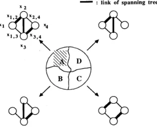
The method for cutting the graph plays an important role in finding the FST’s and in computing the reliability of the DPS. Let us use an example to illustrate this graph cutting method. Consider the DPS graph in Fig. 1 again, we could make sure that all nodes in the DPS should be able to communicate with each other if links x 1 , 2 , 2 2 , 3 , and 2 3 , 4 are all working. This

communicate path ( 2 1 , 2 , 2 2 , 3 , 5 3 , 4 ) is exactly a spanning tree

of the original DPS graph. Let the probability space of the

DPS graph be 1, then it should be equal to the sum of the

following four disjoint probability subgraphs:

1) A probability subgraph that links x1,2, 2 2 , 3 , 2 3 , 4 are all

2) A probability subgraph that link $ 1 , ~ fails,

3) A probability subgraph that link 2 2 , 3 fails but link 2 1 , 2 4) A probability subgraph that link 2 3 , 4 fails but both links This relationship can be depicted in Fig. 2. The whole circle represents the total probability space which is equal to 1. The portion A (shadowed) represents the probability space that the graph has been confirmed to be working and itself is an FST of size 5. While portions B, C, and D are needed to be determined further for finding the FST of size 4. It should be noted that the probability of portion A, B, C, and D is not graphically DroDortional but thev should be summed UD to 1.

working,

must work,

21,~ and 2 2 , 3 must work.

- .

.

link of spanning tree

Fig. 2. The probability space of the original graph G.

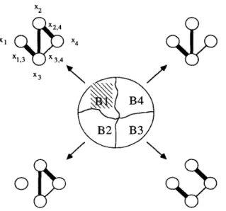
What we need to do next is to determine the probability space of portion B, C, and D. Follow the same idea, we then find a spanning tree from the subgraph representing portion B. The spanning tree tells us that links 2 1 , 3 , ~ 2 , 3 , and 2 2 , 4 must

be up in order to make sure the connection among all four nodes. Thus, the probability of portion B will be the sum of the following four disjoint probability subgraphs:

1) A probability subgraph that links 2 1 , 3 , 2 2 , 3 , ~ 2 , 4 are all 2) A probability subgraph that link ~ 1 , 3 fails,

3) A‘probability subgraph that link 2 2 , 3 fails but link 2 1 , 3

working,

142 IEEE TRANSACTIONS ON PARALLEL AND DISTRIBUTED SYSTEMS, VOL. 3, NO. 2, MARCH 1992

x2

0

n n

Fig. 3. The probability space of the subgraph representing portion B. Fig. 4. The probability space of the subgraph representing portion B3.

4) A probability subgraph that link ~ 2 , 4 fails but both links

This relationship is depicted in Fig. 3. The whole circle rep- resents the total probability space of portion B. The portion B1 (shadowed) represents the probability space that the subgraph has been confirmed to be working and is an FST of size 4.

While portions B2, B3, and B4 are needed to be determined further for finding the FST of size 3. It should be noted that the probability space of portion B1, B2, B3, and B4 is not graphically proportional but they should be summed up to the probability space of portion B (in Fig. 2).

Based on the same concept, we compute the probability subgraphs representing the portion B2, B3, and B4. For example, the probability subgraphs representing portion B3 is depicted in Fig. 4. Again, the probability subgraphs in Fig. 4

should be summed up to the probability space of portion B3. We repeat this process until either the FST of size 0 is obtained,

no available links can be cut, or the subgraph does not contain the required data files for executing the distributed program. For example, Fig. 5 depicts one of the termination conditions of this process.

Once the concept of cutting the graph is understood, we need an appropriate representation scheme to illustrate. Let

si,j be the state of link xi,j of the DPS, where ~ 1 , 3 and X Z , ~ must work.

0 xi,j is down si,j = 1 ~ i , j is UP

{

*

don’t care

with applicable operations based on operator (defined in Section 11-C), then notations LSt, NCt, STt, and LSP, (defined in Section 11-A) can be used to represent the graph cutting process. For example, for the graph of portion

A in Fig. 2, suppose the bit state sequence of links are q 2 , x 1 , 3 , X 2 , 3 , x 2 , 4 , ~ 3 , 4 , we represent it as

LSA =

*****

(the initial graph)

N C A = 00000 (subgraphs can be generated by cutting any

links)

Fig. 5. The probability space of the subgraph representing portion B3.

STA = 1*1*1 (since links x 1 , 2 , ~ 2 , 3 , x 3 , 4 have to be work-

L S P A = 1*1*1 (it is obtained by L S A ST). Likewise, for ing)

the subgraphs B , C , and D can be represented as L S D = 1*1*0

NCB = 00000 NCc = 10000 NCD = 10100

STB = * I l l * STc =

* * * * *

STD =

*****

LSPB = 0111* L S P c = 1*0** L S P D = 1*1*0. LSB = 0**** L s c = I*()**

Since the subgraphs C and D both contain an FST be work- ing (link x 1 , 2 must be working), thus we do not need to find

a spanning tree in subgraphs C and D , so STc =

*****

and

STD = *****. NCc = 10000 guarantee that the subgraph C is

disjoint with the subgraph B , and NCD = 10100 guarantee that the subgraph D is disjoint with the subgraph B and C. It can be inferred that P r ( L S ) = Pr(LSPA)

+

Pr(LSB)

+

P r ( L S c )

+

Pr(LSD) = 1, where Pr(LSc) = Pr(LSPc),Pr(LSD) = Pr(LSPD), and P r ( L S ) can be computed recursively using the graph cutting method introduced above. The informal algorithm for cutting the graph and computing the reliability can be described below.

1) Find a spanning tree from the current graph if necessary and compute STt,

2) Compute the vector L S P t by ST, A LSt, and convert vector LSP, to the probability expression.

3) Cut the current graph according to the vectors STt and

CHEN AND HUANG: RELIABILITY ANALYSIS OF DISTRIBUTED SYSTEMS 143

4) Repeat 1 to 3 to compute each subgraph’s vector LSPt, 5) The reliability of the DPS graph is obtained by unioning all LSPt-vectors that are associated with all the FST’s.

C. The Complete Reliability Algorithm

Once the concept of finding all FST’s and computing the reliability of the DPS is understood, we now present the complete algorithm for finding the FST’s and computing the reliability of the FST.

FST Reliability Algorithm begin

step 1: initialization

t

= original graph ;

TRY = t ; (store the original graph into list TRY) FOUND =

4

LSt = **...* ;

NCt = 00

...

0 ;

F N = Ui FNi (where program i E P V ) ;

R = 4 ;

step 2: generate spanning tree

repeat

2.1 get a subgraph

t from TRY

;

2.2 checking step (check and find spanning tree) remove t from TRY ;

if a FST has been working in

t

then add t to FOUND ; STt =

**...*

;

else find a spanning tree of connected

component i in t such that F A ( 2

F N and P A i

2

P V , and represent it by STt;

LSPt = LSt A STt ;

2.3: cutting step (generate subgraphs) add subgraph(t) to TRY ;

until (TRY =

4)

step 3: compute reliability

for all t in FOUND do

od Reliability = Pr(R) ; R = R V L S P t ; end procedure subgraph(t) begin child = $ ; temp = 4 ;

find each link X k , l with its value in STt = 1 and in /* STt represents all the links of the spanning tree, cut = U ~ , J {xk,l}; /* cut store all the links can be cut

for all xi,j E cut do

NCt = 0 ;

NCt represents all the links cannot be cut */ */

LSnewt =

Lst;

set the state of xi,j in LSnewt to 0; /* cut link xi9j now */

find all links E temp and set those links’ states in temp = temp u{x;,j} ;

LSnewt to 1 ;

find a connected component

i

in

t such

if there are any connected component i found that FA;

2

F N and P A i 2 P V ;

then add newt to child ;

od

return (child) ; end (* subgraph *)

D. The FST Reliability Algorithm with Series and Parallel Reduction

How to speed the reliability evaluation process up is the major concern of the proposed algorithm. The basic principle of speeding the reliability evaluation is to generate correct FST’s with less cutting steps. There are four methods that can be used interchangeably to speed the reliability evaluation. These methods are 1) nodes merged, 2) parallel reduction, 3)

series reduction, and 4) degree-2 reduction.

Nodes merged occurs when a probability subgraph has

bit value 1 in its LS vector. For example, probability

subgraph B3 in Fig. 3 (Section 111-B) with LSB3 =

010** indicates that node x1 and x3 can be merged together since all the subgraphs generated by subgraph

B3 must contain link 21,3. This characteristic is also indicated by the NC vector, N C B ~ = 01 000 in Fig. 3, which tells that link ~ 1 , 3 cannot be cut to obtain its subgraphs. That is the reason why one can get disjoint FST’s using this graph cutting technique.

Parallel reduction occurs when a probability subgraph

contains two or more links between two nodes. With connectivity property, these redundant links can be re- duced to one link.

Series reduction occurs when a probability subgraph has

a node, with node degree = 2, that contains no data file

required for executing the distributed program. Since such a node, after deletion, still does not affect the correct FST generation, we can remove this node and reduce two links that connect to its neighboring nodes into one link.

degree-2 reduction occurs when a probability subgraph

has a node, with node degree = 2, that is not a leaf node of any MFST’s of the current graph. Since this node is not a leaf node of any MFST’s, then the two adjacent links of this node must be working or

fail simultaneously, thus we can remove this node and reduce two links that connect to its neighboring nodes into one link, and copy the data files and programs in this node to its two neighboring nodes.

If node x, satisfies the following checking procedures, then it is defined as a degree-2 reducible node and it will not be a leaf node of any MFST’s.

The procedures of checking if node xn is

a

degree-2 reducible node:

1) delete link xn,i, where node xi is a neighbor node of node x n .

IEEE TRANSACTIONS ON PARALLEL AND DISTRIBUTED SYSTEMS, VOL. 3, NO. 2, MARCH 1992 get a data file Flc from node x,, delete all nodes in the

DPS that contains data file Flc

try to find a FST starting from node

x,,

if there is a FST be found, then node x, is not a degree-2 reducible node and stop these checking procedures.

repeat step 2 to step 3 until each of the data files in node

x,

is considered.

get a program Pk from node x,, delete all nodes in the

DPS that contain program Plc.

try to find an FST starting from node x,, if there is an FST be found, then node x, is not a degree-2 reducible node and stop these checking procedures.

repeat step 5 to step 6 until each of the programs in node x, is checked.

recover link z,,~ and delete the other link x n , j , where node xj is another neighbor node of node

x,.

repeat step 2 to step 7

10) if the checking procedures is not stopped in the middle In the following, we use an example to illustrate these reduction methods. Suppose there is a subgraph generated as shown in Fig. 6(a), we need to compute the reliability of program 1 which requires data files F1, F 2 , F3, and F 4 for completing its execution. Suppose the bit state sequence of links are x 1 , 2 , ~ 1 , 3 ~ X Z , ~ ~ ~ 2 , 4 , x3,5, x4,5, and the following reduction steps are applicable for speedup the correct FST generation.

Step 1: Since link x1,2 can no longer be cut and must be up for the rest of its subgraph generation ( L S = l**O**), we apply nodes merged reduction on nodes x1 and x2. The

resulting subgraph(b) is shown in Fig. 6(b).

Step 2: A parallel reduction can be applied on the resulting subgraph (from step 1) since links x 1 3 and ~ 2 , 3 are parallel.

The new resulting subgraph(c) is shown in Fig. 6(b). Step 3: A series reduction occurs since node 2 5 contains no data files for the execution of program 1. The new resulting subgraph(d) is shown in Fig. 6(b).

Step 4: A degree-2 reduction occurs since node 2 3 is not a leaf node of any MFST's. The final subgraph(e) after these reductions is also shown in Fig. 6(b).

Once these reduction techniques are understood, we need new representations for computing STt and LSnewt

.

These new representing schemes are discussed below.

1) STt and LSnewt representation in parallel reduction:

Let two links x , , ~ and xk,l in graph t be parallelly reduced

into itself be one of the links in the spanning tree we found, and the bit state sequence of both STt and LSnewt be (.

.

9 x z , j x k , l

. .

.), then

a) the state of STt after reduction will be

(.

.

. l l . . . ) V (.

.

. l o . . .) V (.

.

.Ol

. .

.), and b) the state of LSnewt (newt is a child of

t )

after

reduction will be (.

.

.OO

.

.

.).

This can be seen from the fact that x : , ~ = ~ , , ~ x k , l . It implies that if link x : , ~ is working then either link x 2 , 3 or 2 k , l must be working, and if link fails then both links x , , ~ and 2 k , I must have failed.

2) STt and LSnewt representation in series reduction or in

and X I F I in graph

then

x,

is a degree-2 reducible node.

degree-:! reduction: Let two links x,

m m m

I

4

FA

_ _ _ _ _ _ _ _

'2.4

2

FA F4 _ - _ - : failure FA FI x2,3 x4,5

-

: working X1 PRG PI

-

:don'tcare x133 FA F3 FA F5 FN1 = (Fl,FZE3.F4} x3.5 x3 x5 LS = 1**0** NC = 1 0 0 0 0 0

x1 and x2are merged parallel reduclion series reduction for degree-2 reduction for

for x1.3 mdX2,3 XS. '5,s mdx4.5 x39x1,3 & 9 , 4

(step 1) (step 2) (step 3) (step 4) (b)

Fig. 6. (a) A subgraph during reliability evaluation process. (b) Reduction

for subgraph of (a).

t be series reduced or be degree-2 reduced into

xi,j, xi,j

itself be one of the links in the spanning tree we found, and the bit state sequence of both STt and LS,,,t be

(.

.

. ~ ~ , ~ z k , l . . .), then

the state of STt after reduction will be (.

.

.

11

. .

.).

the state of LSnewt (new, is a child of

t )

af- ter reduction will be (.

.

. O O . . .) V (.

.

. l o . .

.) V This can be seen from the fact that x : , ~ = xi,j nxk,z. It also implies that when link x : , ~ is working then both links xi,j

and x k , J must be working, and if link x : , ~ fails then either link xi,j or x k , l must be failed.

3) STt and LSnewt representation in the combination of

both series and parallel reduction or degree-2 and par- allel reduction: There are several combination reduction cases that may occur during the FST generation. For ex- ample, links xi,j and xk,j, firstly, are parallelly reduced into xi,j, and then and xm,, are series or degree-2 reduced into x&. Let the bit state sequence of both STt and LSnewt be (.

. .

x i , j X k , l x m , n . . .), then

the state of STt after reduction will be (. . . 111

. .

.)

a) b)

(.

.

.Ol

. .

.).

a)

v

(.

.

. l O l . . .)

v(.

.

. 0 1 1 . . .).

b) the state of LSnewt (newt is a child of

t )

af- ter reduction will be (.

.

,001.. .) V (.

.

. l l O . . .)

This can be seen from the fact that x : , ~ = (xi,jUzk,l)nz,,,. Other combination cases can be represented in the same way.

CHEN AND HUANG: RELIABILITY ANALYSIS OF DISTRIBUTED SYSTEMS

The FST reliability algorithm can be incorporated with these techniques to speed up the reliability evaluation. The complete FST reliability algorithm with series, parallel, and degree-2 reduction is listed below.

FST-SPR algorithm

begin

step 1: initialization t = original graph;

TRY = { t } (store the original graph into list TRY) FOUND =

4

LSt =

* *

. . . *; NCt = 00

. . .

0;

FIV = U, F N I (where program i E Pk') ;

R = 4 ;

step 2: generate spanning tree

step

end

repeat

2.1 get a subgraph t from TRY ; 2.2 reduction step

repeat

series-reduction(t) ; degree-2-reduction(t) ; parallel-reduction(t) ;

until no reduction occurs

remove t from TRY;

if an FST has been working in t 2.3 checking step

then add t to FOUND;

else find a spanning tree of connected component / in f such that

F A ,

2

F N and P A ,

2

P V , and repreqent i t by STt with the new representation discussed in Section 111-D ;

ST,=*"

. . . "

LSPt = LSt A STt ;

2.4 cutting step

add subgraph(t) to TRY ;

until (TRY =

4)

3: compute reliability

for all t in FOUND do

od Reliability = Pr(R); R = R V LSP,; procedure subgraph(t) begin child = d, ; temp =

4

;

find each 3'1; 1 where r1; cut =

u1;

I { & 1 ) ;

for all ic, cut do

E stree and the state of .L'k in N C t = 0 /* cut store all the iinks can be cut */ LS,,ult = L S t ;

set the state of x, in LSILevt to 0; /* cut links, now */ find all links which temp and modify LS,,, + with these links by new representation discussed in Section 111-D;

merge(newt,temp) ; temp = temp ~ { r , 3 } ;

find a connected component a in t such that F A , 2 F N and P A , 2 P V ; if there are any connected component z found

146 IEEE TRANSACTIONS ON PARALLEL AND DISTRIBUTED SYSTEMS, VOL. 3, NO. 2, MARCH 1992

then add newt to child;

od

return (child);

end (* subgraph *) procedure series-reduction(t)

begin

for all node xi in t do

if degree of xi = 2

then if ( F A i

n

F N =

4

) AND (PRG;

n

PV =

4

)

then delete node xi and link xi,j ( x j is one neighbor of x i ) from

t ;

if X k , j exists

then rename X k , i to x i , j ;

else rename X k , i to X k , j ;

record X k , j (or x i , j ) be series reduced by X k , ; and x i j ;

od

end (* series-reduction *)

procedure parallel-reduction(t)

begin

for all node xi in t do

for all xi’s neighbors xj do

if there are two links x,,j and x : , ~ between

x;

and x j ;

then record parallel-reduction on link x;,j and x : , ~ ; delete x : , ~ from t ; od od end (* parallel-reduction *) procedure degree-2-reduction(t) begin

for all node x , in t do

if deg(x,) = 2

then for all the adjacent link x , , ~ of node x , do delete link x , , ~ ;

repeat.

get a data file F k from FA, or a program

Pk

from PRG,, delete all nodes that contain data file F k or Pk in subgraph t ; try to find a FST starting from node x,,

if there is a FST be found,

then node x , is not a degree-2 reducible node and break until all F k or Pk reside in node x , has been considered.

recover link x , , ~ ;

od

if node x , has not been determined is a degree-2 reducible node or not then delete node x , and link x,,, ( x J is one neighbor of x , ) from

t;

if X k , , exists

then rename xk,, to x;,,; else rename X k , , to xk,, ;

P k , j (or Pi,, ) = pk,z

*

Pz,, ;

FAk = FAk U FA,; PRGk = PRGk U PRG, ;

F A , = F A , U F A , ; PRG, = PRG, U PRG, ;

od end

procedure nodes-merged(t,temp)

begin

147

CHEN AND HUANG; RELIABILITY A N A L Y S I S OF DISTRIBUTED SYSTEMS

F A i = F A i U FA,; PRGi = PRGi A PRGj; delete node x j and link x i j ; parallel-reduction(t) ;

od

end (* nodes-merged *)

IV, RELIABILITY ANALYSIS OF DPS USING THE FST AND FST-SPR RELIABILITY ALGORITHMS

A . Examples

In this section we use the FST and FST-SPR reliability algorithms to evaluate some distributed processing systems.

Example I: Consider the simple DPS example in Fig. 1 again, we use the FST reliability algorithm to analyze the DPR1. We use the Distributed Program Reliability

i

(DPR,) to describe the reliability of the distributed program i running under the DPS and Distributed System Reliability (DSR) to describe the overall reliability of the distributed system.

The splitting snapshot of subgraphs generated by the FST reliability algorithm is illustrated in Fig. 7.

To compute the reliability, we simply sum all the disjoint terms represented by vectors U P t . Let Pr(i) be the probability subgraph i, then Pr(A) = Pr(1 *1

*

1) Pr(B) = Pr(Olll*)

+

Pr(1)

+

Pr(1c) = Pr(Olll* V 0110* V 01001 VO1011 V 00 101 V = Pr(Olll*

v

0110* V 010*1

v

00 101 V 0011* 0011*

v

00 011

v

00 001) V O O O l l

v

00001) = P r ( O l l l * vo110*

v

010*1

v 00

101

v

0011*

v

OOO*l) = Pr(Oll** V 010

*

1 V 00 101 V 0011* V 000*1) = Pr(Oll** V 0*0*1 V 00 101 V 0011*) Pr(C) = Pr(l*O**) Pr(D) = Pr(l*l*O) DPRl = Pr(A)

+

Pr(B)

+

Pr(C)

+

Pr(D) = Pr((1

*

1

*

1) V (011** V 0*0*1 V 00 101 V = Pr(1

*

1

* *

V 011** V 0*0*1 V 00 101 V = Pr(l**** 011** 0*0*1 00 101 OOll*) = P1,2

+

41,2P1,3P2,3

+

41,2!?2,3P3,4 OOll*)

v

(l*O**)

v

(1

*

1

*

0)) 0011*

v

l*O**) +Q1,2Q1,3P2,3q2,4P3,4

+

Q1,241,3P2,3P2,4 If we assume all the links have the same reliability 0.9, then DPRl is equal to 0.99891.

For evaluating the DSR, the FN = {Fl, F2, F3,

F4). Applying the same algorithm, we obtain

DSR

=

P1,2P2,3

+

P1,2P1,3q2,3

+

pl,Zq1,3q2,3P2,4P3,4

+

91,2P1,3P2,3

+

41,242,3P2,4P3,4 +Ql,291,3P2,3Q2,4P3,4 +41,241,3P2,3P2,4. Again, if we assume all the links have the same reliability 0.9, then the DSR is equal to 0.9963. These results are correctly matched

DPRJ = Pr( 11**1 V 011*1 V *01*1 V 0*011 V 10011

v

11*10

v

*0110

v

01110)

Pl,2P1,3Q2,3Q2,4P3,4 + P1,2P1,3Q2,3P2,4Q3,4 = 0.98658 (with = P2,3P2,4 + P2,342,41)3,4 + 42,3P2,41)3,4 + the assumption of reliability 0.9 for all links)

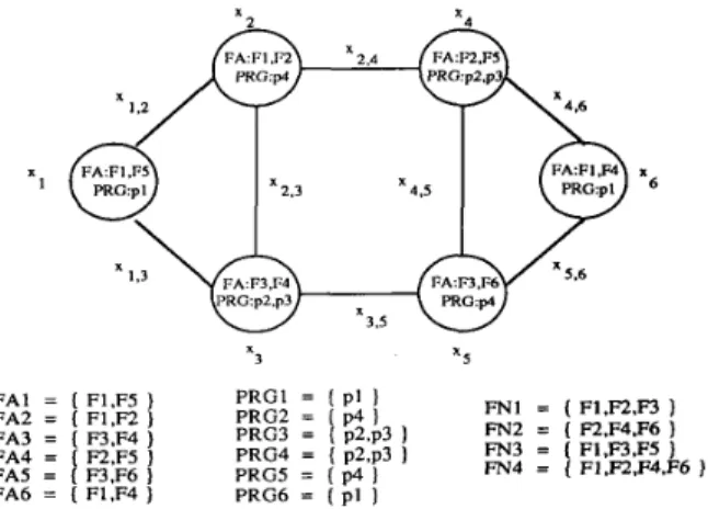
Example 3: Considering the DPS shown in Fig. 9, it contains

six processing elements and the detailed information of each node is given in sets of F A j , PRGj, and F N j .

Again, we want to compute the DPRl and DSR of the DPS. Applying the same reliability program, we get DPRl = 0.9995076 and DSR = 0.9975515 under the assumption of all links with reliability 0.9

B. Other Evaluation Results

Reliability problems listed in Section 11-C are addressed here. Fig. 10 presents the single distributed program reliability (DPR1, DPR2, DPR3, and DPR4) running under the DPS in Fig 9. This analysis can help us to understand the reliability of each program under a certain data files distribution such that an optimal data files distribution for balancing each program’s reliability can be validated.

Fig. 11 presents the reliability of two or more distributed programs running together under the DPS in Fig. 9. This anal- ysis will help us to assign programs into different processing elements. An intended programs assignment to achieve higher reliability can be validated through this analysis.

Fig. 12 presents the reliability of one or more copies of the program 1 running together starting from different sites. The resulting reliability is under the DPS graph in Fig 9. This analysis will help us to make sure if the program under execution has reached the required reliability.

Fig. 13 presents the DPRl under the choices of different user sites. This analysis will help users to choose a better site to execute a certain program.

C. The Correctness and Time Complexity of the Algorithm Theorem I : Given a graph G = { N ,

E}

where N = {x1,52,

..

.

,x,} is a set of nodes, and E = (L1, L z , . . .

,

Ln} is a set of links. Let

L

= { L1, L2,.

,

Lm-l} E

E

be a set of links representing a spanning tree of G, then the probability space of the graph G can be expressed as the following disjoint terms.

Pr(G) = ~ 1 ~ 2 . . -pm-1Pr(G1)

+

qiPr(G2)

+

plq2Pr(G3)

+

*

. .

+

~ 1 ~ 2 . * .pm-zqm-1Pr(Gm) (1)

where pi denotes the probability that L; is working, q; denotes the probability that L, is failure, G I denotes G with L1, L2,

. .

,

L,-l is working. G2 denotes G with L1 is failure. G3 denotes G with L1 is working and L2 is failure,

.

. .

G,

denotes G with L1, L 2 , . - - , Lm-2 is working and L,-1 is failure.

Proof: By factoring theorem (or conditional probability). with the results in [12] and [13].

Example 2: Considering the DPS graph in Fig. S(a), we will

use the FST-SPR reliability algorithm to compute the DPR3. The splitting subgraphs generated by the FST-SPR reliability algorithm is illustrated in Fig. 8(b).

Pr(G) = qiPr(GIFi)

+

p i P r ( G ( E ) = qiPr(Gi)

+

piPr(Gi) where

Fi

denotes the event that Li is failure, F, denotes the event that Li is working, G, denotes G with

Li

is failure,

GI

148 IEEE TRANSACTIONS ON PARALLEL AND DISTRIBUTED SYSTEMS, VOL. 3, NO. 2, MARCH 1992

-

: link of spanning wee

.$.

LS = ***** NC = 00000 ST = 1*1*1 L S P = 1*1*1

0

O O P

NC = 1OOM) N C = 10100 ST = ***** LSP = 1*1*0 N C = 00000 ST = *111* LSP = 011 1* ST = ***** LSP = l*O**

/@\

0,

0

0

Ls =oooo* NC =oOOMl ST = ****I LsP =00001

I

0

0

0

0

1s =ooooo NC =WOW Fail

0

LS =00010 Ls =oo*** NC =OW00 NC =00010 yr = * t i l * Fail LSP = 001 I’

/ \

/ \

LS =OW** LS =0010* NC = 00000 ST = * * * I 1 ST =**l*l NC = 00100 LSP = 0001 L I S P = 00101

I

I

=0100* Ls =01010 NC =01000 NC =01010 ST = *l**l Fail I S P =01001

0

@

o g , ,

b

0

LS =oOlW Ls =01000 Fail Fail NC =00100 NC =01000 Fig. 7. T h e splitting snapshot of the original graph.

If we choose L1 be the first factor, then If we repeat the same action, then P r ( G h - l ) can be

expressed as Pr(G) = qlPr(G2)

+

plPr(G/,).

P r ( G L - l ) = q,-lPr(Gm)

+

prn-lF’r(GL) Obviously, Pr(Gh) can be expressed in the same way, thus

we choose La be the second factor, then where G, denotes G h P l with L,-1 is failure, G L denotes GL-l with L,-1 is working.

CHEN AND HUANG: RELIABILITY ANALYSIS OF DISTRIBUTED SYSTEMS X PRGZ: P1 149 PRGI: F 2 X 1.3 F A F 3 3.4 PRG3: P3 3 PRGl = I p2 1 PRG2 = 1 PI 1 PRG3 = [ P3 1 PRG4 = ( P2 1

-

: Unk of rpannlng lree 11 CM be wrler reduced

xI,2and x1.3 are series reduced Into x2.3'

1

,s =

*....

NC = 00000 ST = 1 1 * * 1 v 011.1 v '01.1 LSP = 11-1 v 011.1 v *01*1 _{x 3 Is merged Inlo 12} x3.4 I S CUI x2*3-* IS>

40

Ls = 11-0 " 011.0 v *01*0

%

1

NC = 00100 ST E ***1*

d

LSP 11-10 v w110 v 01110 x, Is a degree.2 reduclble node

x2.4 M d x3.4 are degree-2 reduced Into X Z , ~ ' q 4 ia cut

1

0

0

Ls = 11.00 v OllOO v *0100

8

~ 2 . 4 . = x 2 - 4 n x3.4 x2.4' Ls = 0.0- v 100.. NC = 00000 ST = ***I1 LSP = 0'011

"

10011 N C I 00100 Fall X2,4' I s CUL

I

0

0

Ls E 0.001 v 1000' NC = 00000 Fall @)

150 lEEE TRANSACTIONS ON PARALLEL AND DISTRIBUTED SYSTEMS, VOL. 3, NO. 2, MARCH 1992

f plp2p3q4Pr(G5)

+

‘ ‘ ’

+

P1P2 * ’ ‘pm-2qm-lPr(Gm)

x

2 X

+

PlP2.

.

% - l P 4 G 6 ) (2)

where G L denotes G with L1, L2, e

. .

,

Lm-l is working, G2

denotes G with L1 is failure, G3 denotes G with L1 is working and L2 is failure,

.

. .

Gm denotes G with L1, L2,

.

’

,

Lm-2 is working, and L,-1 is failure. Let G1 (in equation 1) = G L [in (2)], then (1) = (2). Thus, Theorem 1 is proved. Q.E.D.

Proof: To prove FST reliability algorithm correct, we

transfer this problem into the one shown in Theorem 1. The

Theorem 2: The FST reliability algorithm is correct.

3 x 5 PRGl = ( p i 1 PRG2 = [ p4) PRG3 = [ ~ 2 . ~ 3 ) FN2 = F2,F4.F6 PRG4 = ( ~ 2 . ~ 3 ) PRG5 = ( p4 I PRG6 = [ pl 1 F N l = (Fl,FZ,F3 ) FN3 FlV4 = = ( ( F 1 m m Fl.FZ.F4,F6 ) novelty of the FST reliability algorithm lies in its graph cutting

method. The cutting technique works exactly the same way as

Fii

5

I

Fig

Fi:

1

/

z;F;

the enumeration of all disjoint terms in Theorem 1. Recalling

_{Fiz 1}

_/

_E;;:

1

the probability subgraphs in Fig. 2, the original graph is

partitioned into four probability subgraphs A, B , C, and D

by the cutting technique. By analogizing these probability subgraphs to the terms in Theorem 1, we found that the original Probability graph represents Pr(G); subgraph A represents P I , ~ P ~ , ~ P ~ , ~ P I ( G A ) ; subgraph represents q i , 2 P r ( G ~ ) ; sub- graph

c

represents P I , ~ Q ~ , ~ P ~ ( G c ) ; subgraph

D

represents P1,2P2,3q3,4Pr(GD). More precisely,

Fig. 9. A DPS with six processing elements.

no data files required for executing the distributed program, and each degree-2 reduction occurs when a graph has a node with node degree=2 and this node is not a leaf node of any MFST’s. None of these cases has violated the disjoint property and FST definition. Thus, the’ FST-SPR reliability algorithm P ~ ( L S G ) = P ~ L S P A ) + P ~ ( L S B ) +Pr(LSc) +Pr(LSD) is also correct. Q.E.D.

Theorem 4: The FST and FST-SPR reliability algorithms guarantee no replicated FST’s to be generated during the reliability evaluation.

Proof: Suppose there are two or more replicated trees

generated by the FST or FST-SPR reliability algorithm, then both FST and FST-SPR algorithms will generate nondisjoint probability subgraphs. This is contradiction with Theorem 1 which generates the disjoint probability space of each term. Thus, the FST and FST-SPR algorithm guarantee no replicated FST’s to be generated during the reliability eva1uation.Q.E.D. Unlike the time complexity analysis in the K-graph prob- lem, which is statically dependent on the given k-terminal = P r ( 1

*

I

*

I)

+

Pr(O

* * *

*)

+

Pr(1

*

O

*

*)

+

P r ( 1

*

1

*

0)

= P1,2P2,3P3,4Pr(Ga)

+

ql,2Pr(Gb)

+

P1,2q2,3Pr(Gc)

+

P1,2P2,3q3,4Pr(Gd) = Pr(G).

The probability of these subgraphs can be computed recur- sively based on the graph cutting technique again to obtain the probability of its subgraphs. The FST reliability algorithm uses such cutting technique to compute the reliability of any size and any data distribution DPS. Thus, generalized terms will be

Pr(LSG) = Pr(LSP1)

+

Pr(LS2)

+

+Pr(LS3).

. .

+

Pr(LSn) = P1,2P1,3p2,3.. .Prn,nPr(Gl)

+

q1,2Pr(G2) f q1,2Pr(G2)P1,2q1,3Pr(G3)

+

’ ’ ‘

+

P1,2P1,3P2,3 ‘ ’ “?m,nPr(Gn) = Pr(G).

By such analogous, we have successfully transferred the FST reliability algorithm into the problem in Theorem 1. Since

Theorem 1 is correct, therefore, Theorem 2 is also correct. Q.E.D.

Theorem 3: The FST-SPR reliability algorithm is correct. Proof: We have shown the correctness of the FST relia-

bility algorithm. What we need to show is the correctness of

nodes merged, series, parallel, and degree-2 reductions. These

reduction techniques are true intuitively. Since each nodes merged occurs when a particular link in the graph cannot be cut in the rest of its subgraphs generation, each parallel reduction occurs when a graph with two or more links are connected between two nodes, each series reduction occurs when a graph has a node with node degree = 2 contains

connection, the time complexity of distributed program relia- bility problem is dynamically bound to the data files required for each distributed program. The time complexity of the algorithms presented in [12]-[14], in worst case, can generate as many as ( n - l)(e-l) intermediate trees, where TI denotes

number of nodes and e is the maximum in-degree of a node in the graph. However, in practical condition, such case never occurs since once an FST is found the tree expansion is stopped. The proposed FST algorithm uses the graph cutting technique with incorporated series and parallel reduction to speed the FST generation. The time complexity is quite difficult to quantify since the number of links and nodes may be reduced or merged during the evaluation process. However, by common reasoning, the complexity should be less than that of the algorithms presented in [12]-[14]. One of the good ways to compare the proposed FST algorithm with existing algorithms [12]-[14] will be based on the intermediate trees (or subgraphs) generated during the whole reliability evaluation process. In this way, one can tell how much memory space and time unit required for their algorithms to run the distributed program. We will present some such comparison results in Section IV-D.

CHEN AND HUANG: RELIABILITY ANALYSIS OF DISTRIBUTED SYSTEMS 151

reliability

reliability

reliability of links

Fig. 10. Reliability of each DPR.

A 0 A U 0 DPRl DPRP DPR3 DPR4 P1 &P2 Pl&P2&P3 p1 &p2&p3&p4 reliability of links

Fig. 11 Reliability of two or more programs running together.

D.

Algorithms Comparison

Unlike Kumar’s algorithm [12], [13] required two passes

to formulate the reliability of the DPS, i.e., to generate all MFST’s first and then use reliability analysis program such as SYREL [ll] to compute the reliability DPR and DSR,

our algorithm requires only one pass to generate the FST’s and compute the reliability. Kumar’s algorithm [12], [13]

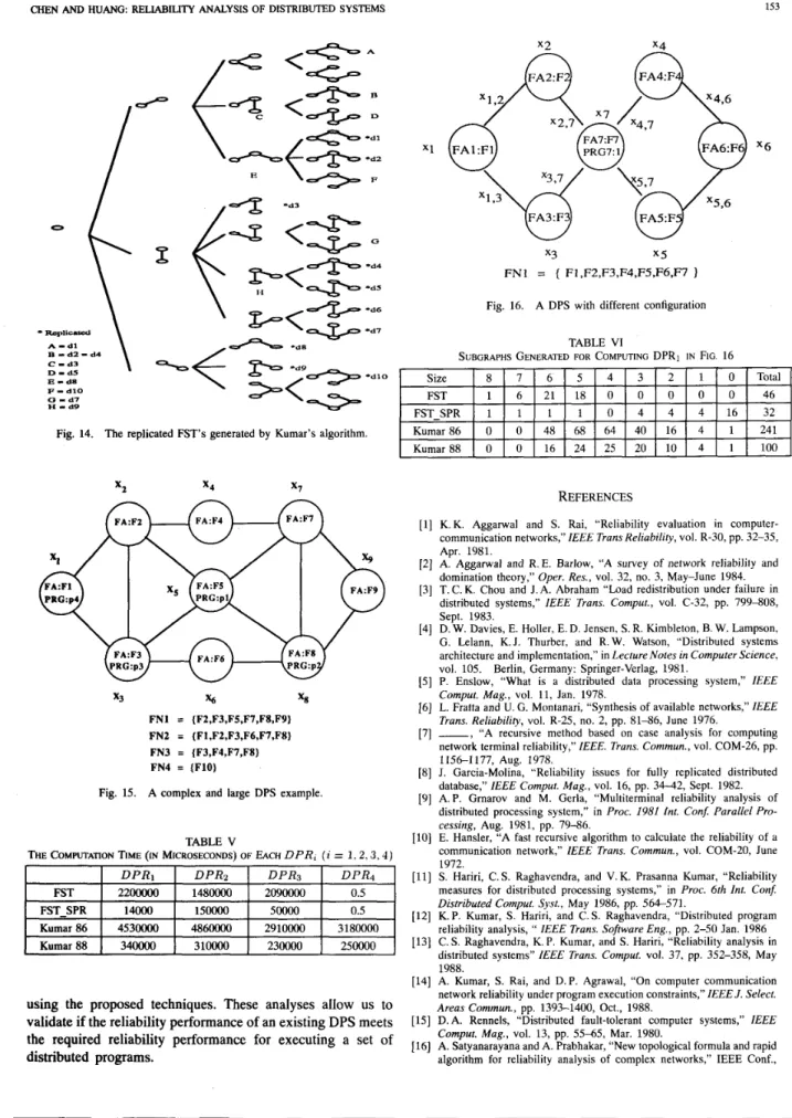
has potential to generate a lot of replicated MFST’s during the MFST’s generating process. Thus, it has to pay extra effort to remove the replicated trees. Our algorithm guarantees no replicated FST’s to be generated during the subgraphs generating process. Fig. 14 presents the replicated FST’s

generated while computing the DPRl in the DPS in Fig. 8 by using Kumar 86’s algorithm.

Although the algorithm presented in [14] also uses one pass

to generate FST (by matrix representation) and compute the reliability, it only addresses a single distributed program issue. For problem statements such as 2, 3, and 4 listed in Section II- C, their algorithm cannot solve such problems. In general, the difference between the FST algorithm and existing algorithms [ 121 -[ 141 lies in that existing algorithms use the concept of tree growing while the FST algorithm uses the concept of graph cutting.

Since the time and space required of these algorithms are bound by the number of subgraphs (or trees) generated during the FST generating process, we present some sampling DPS graphs for comparison.

reliability 1 0 . 9 0.8 0.7 0 . 6 0.5 0.4 0.3 0 . 2 0.1 0 0 0.1 0 . 2 0 . 3 0 . 4 0 . 5 0 . 6 0 . 7 0 . 8 0 . 9 1 reliability of links * X l 0 ~ 1 . ~ 6 -x- XI ~ 2 . ~ 6 or xl.x2,x4.x6 or x i , ~ 2 , ~ 3 , x 4 . x 6 or x l . x 2 . x 3 . x 4 . x 5 . ~ 6

Fig. 12. DPRl with several copies of distributed program one.

reliability I 0.9 0.8 0.7 0.6 0.5 0.4 0.3 0.2 0.1 0 n X 2 01 X3 01 X4 OT 0 0.1 0.2 0.3 0.4 0.5 0.6 0.7 0.8 0.9 I reliabili~y of links

Fig. 13 The DPRl under different user sites

Table I presents the best case of our algorithm. It should be noted that the current algorithms in [Kumar 86, 881 cannot

compute the reliability of a distributed program with no data files in the distributed networks. Results in Table I are based on the modification of their algorithms to take care such problem. Table 11, 111, and IV show the cases for the reliability analysis of programs 1, 2, and 3 respectively. The size of the graphs

(or trees) is measured by the number of links.

For the actual execution time comparison, we present the

DPR, ( i = 1 , 2 , 3 , 4 ) analysis based on the IBM RISC

System/6000 under single user environment to collect exe- cution time. All four algorithms are structured to have the same I/O activities to insure the fairness of the comparison. These four programs are listed in the Appendix in [19]. It is

clear that the FST-SPR algorithm has the best performance while Kumar 86’s algorithm is the worst one. This result justifies that the tedious and time consumming procedures to check replicated trees and to remove them from the TRY-LIST dominate the whole computation time. The computation time (in microseconds) of the DPR, are listed in Table V.

Overall speaking, the FST algorithm has the following advantages compared that with existing algorithms.

1) The FST algorithm generates less subgraphs and thus

saves the computation time and space. Unlike Kumar’s algorithm [12], [13] which has potential to generate

replicated FST’s which requires a tedious checking process, our algorithm guarantees no replicated FST’s to be generated during the subgraphs generation.

2) With the incorporation of nodes merged, series, degree-

152 IEEE TRANSACTIONS ON PARALLEL AND DISTRIBUTED SYSTEMS, VOL. 3, NO. 2, MARCH 1 9 2

F S T - S P R 1 Kumar 86

Kumar 88

TABLE I

SUBGRAPHS GENERATED FOR COMPUTING D P k

Size

1

1 4 1 1 3 1 1 2 1 1 1 1 1 0 1 9 1 8 1 7 1 6 1 5 1 4 1 3 1 2 1 l I O I T o t a l FST

I

1 l o l o l o l o l o l o

l o l o l o l o l o l o l o l o l

1 0 0 0 0 0 0 0 0 0 0 0 0 0 0 1 0 0 0 0 0 0 1984 2206 1144 396 112 32 8 2 1 5885 0 0 0 0 0 0 640 828 499 206 67 22 7 2 1 2272 FST-SPR Kumar 86 Kumar 88 TABLE I1

SUBGRAPHS GENERATED FOR COMPUTING DPRl

1 0 0 0 1 1 2 2 5 9 10 15 15 18 109 188

0 0 0 0 0 0 1260 2844 2092 884 284 80 20 4 1 7469

0 0 0 0 0 0 321 863 748 373 139 46 14 4 1 2509

TABLE 111

SUBGRAPHS GENERATED FOR COMPUTING DPR2

Size

I

14 I 1 3 I 1 2 I l l I 1 0

I

9

I

8

I

7

I

6 1 5 I 4 1 3 1 2 1 1 I O ITotal

FST

I

1

I

8

I

33

I

96

I

232

I

451

I

651

I

646

I

308

I

52

I

0

I

0

I

0

1

0

I

0

I

2478

TABLE IV

SUBGRAPHS GENERATED FOR COMPUTING DPR3

bility algorithm, our reliability evaluation algorithm for distributed program is much faster and requires less memory space.

3) The FST reliability algorithm addresses some distributed program related problems which were not addressed by some other techniques.

4) The FST Reliability evaluation algorithm is simple and consistent through a special union operation on all vectors L S P representing the probability space of each FST. Our algorithm is a unified approach for both generating FST’s and computing the reliability of the DPS.

Fig. 16 shows a different DPS configuration for more comparisons and the results are listed in Table VI.

V. CONCLUSION

Distributed Processing system provides cost-effective ways for improving computer system’s performance such as through- put, fault-tolerance, reliability, and so on. The reliability analysis of the DPS becomes an important issue. Traditional approaches for the reliability analysis of computer networks may not be directly applicable for the DPS for that the effects

of redundant data files and programs are not captured in these methods. To overcome these limitations, new method should be proposed. In this paper, we present a unified algorithm to generate FST’s and to compute the reliability of the DPS. To speed up the reliability evaluation, nodes merged, series,

degree-2, and parallel reduction techniques are incorporated

into the algorithm.

The algorithm presented in this paper is based on the concept of graph cutting to generate FST’s. The reliability computation is simple and consistent through a special union operation on all vectors LSP representing the probability space of each FST. The algorithm guarantees no replicated FST’s to be generated. The proposed algorithm outperforms existing algorithms in terms of less time and space requirement. This can be evidenced from the various comparisons shown in Section IV-D. It should be mentioned that the best case performance of Kumar’s algorithms is that all the data files required for the program to be executed are collided at one same node that also contains the executed program. In fact, this case is not like to happen in the distributed process- ing system which usually evenly distributed the available resources @rograms,data files). Several DPS related problems which are not addressed by other algorithms are studied here

CHEN AND HUANG RELIABILITY ANALYSIS OF DISTRIBUTED SYSTEMS 153 FST FST SPR * R e p l i E d A - d l E - d Z - d 4 C - d 3 D - d 5 E - d a DPRl DPR2 DPR3 DPR4 2200000 148oooO 209oooO 0.5 14000 15oooO 5 m 0.5 P

-

d10 0 - d 7 H

-

d9

x

5 *d3

=+-

Fig. 14. The replicated FST’s generated by Kumar’s algorithm.

x4 x3 x,

xs

FNl = (FZ,F3,FS,F7,FS,F9) FN2 = (FI,F2,F3,F6,F7,FS) FN3 = (F3,F4,F7,FS) FN4 = (F10)

Fig. 15. A complex and large DPS example.

TABLE V

THE COMPUTATION TIME (IN MICROSECONDS) OF EACH D P R , ( i = 1 , 2 , 3 , 4 )

FA4:F

W

W

x3 x 5

F N l = ( FI,F2,F3,F4,F5,F6,F7 ) Fig. 16. A DPS with different configuration

TABLE VI

SUBGRAPHS GENERATED FOR COMPUTING DPRl IN FIG. 16

Kumar86 1

I

Kumar88

I

0

I

0 I 1 6 I 2 4 I 2 5 I 2 0 I 1 0

I

4

I

1

I

I

0

I

0

I

48

I

68

I

64

I

40

1

16

I

4

I

241 100

I Kumar 86 I 453oooO I 486oooO I 291oooO I 3180000 I Kumar88

I

340000

]

31oooO

I

23oooO

1

25oooO

using the proposed techniques. These analyses allow us to validate if the reliability performance of an existing DPS meets the required reliability performance for executing a set of distributed programs.

REFERENCES

[ l ] K.K. Aggarwal and S. Rai, “Reliability evaluation in computer- communication networks,” IEEE Trans Reliability, vol. R-30, pp. 32-35, Apr. 1981.

[2] A. Aggarwal and R.E. Barlow, “A survey of network reliability and domination theory,” Oper. Res., vol. 32, no. 3, May-June 1984. [3] T. C. K. Chou and J. A. Abraham “Load redistribution under failure in

distributed systems,” IEEE Trans. Comput., vol. C-32, pp. 799-808, Sept. 1983.

[4] D. W. Davies, E. Holler, E. D. Jensen, S. R. Kimbleton, B. W. Lampson, G. Lelann, K. J. Thurber, and R. W. Watson, “Distributed systems architecture and implementation,” in LectureNofes in Computer Science, vol. 105.

[SI P. Enslow, “What is a distributed data processing system,” IEEE

Comput. Mag., vol. 11, Jan. 1978.

[6] L. Fratta and U. G. Montanari, “Synthesis of available networks,” IEEE

Trans. Reliability, vol. R-25, no. 2, pp. 81-86, June 1976.

[7] -, “A recursive method based on case analysis for computing network terminal reliability,” IEEE. Trans. Commun., vol. COM-26, pp. 1156-1177, Aug. 1978.

[8] J. Garcia-Molina, “Reliability issues for fully replicated distributed database,” IEEE Compuf. Mag., vol. 16, pp. 34-42, Sept. 1982. [9] A. P. Grnarov and M. Gerla, “Multiterminal reliability analysis of

distributed processing system,” in Proc. I981 Inf. Con$ Parallel Pro-

cessing, Aug. 1981, pp. 79-86.

[lo] E. Hansler, “A fast recursive algorithm to calculate the reliability of a communication network,” IEEE Trans. Commun., vol. COM-20, June 1972.

[ l l ] S. Hariri, C. S. Raghavendra, and V. K. Prasanna Kumar, “Reliability measures for distributed processing systems,” in Proc. 6th Inf. Conf:

Distributed Compuf. Syst., May 1986, pp. 564-571.

[12] K. P. Kumar, S. Hariri, and C. S. Raghavendra, “Distributed program reliability analysis, “ IEEE Trans. Sofrware Eng., pp. 2-50 Jan. 1986

[I31 C. S. Raghavendra, K. P. Kumar, and S. Hariri, “Reliability analysis in distributed systems” IEEE Trans. Compuf. vol. 37, pp. 352-358, May 1988.

[14] A. Kumar, S. Rai, and D.P. Agrawal, “On computer communication network reliability under program execution constraints,” IEEEJ. Select.

Areas Commun., pp. 1393-1400, Oct., 1988.

[15] D. A. Rennels, “Distributed fault-tolerant computer systems,” IEEE Cornput. Mag., vol. 13, pp. 5 5 4 5 , Mar. 1980.

1161 A. Satyanarayana and A. Prabhakar, “New topological formula and rapid algorithm for reliability analysis of complex networks,” IEEE Conf.,

154 IEEE TRANSACTIONS ON P A R W E L A N D DISTRIBUTED SYSTEMS, VOL. 3, NO. 2, MARCH 1992

1978.

1171 A. Satyanarayana, “A unified formula for analysis of some network reliability problems,” IEEE Trans. Reliability, vol. R-31, pp. 23-32, Apr. 1982.

[18] J. A. Stankovic, “A perspective on distributed computer systems,” IEEE Trans. Cornput., vol. C-33, pp. 1102-1115, Dec. 1984.

1191 D. J. Chen, “RFST A distributed system reliability analysis program,” TR-91-004, Comput. Sci. and Inform. Eng. Dep., National Chiao Tung

Univ., 1991. Association.

Tien-Hsiang Huang received the B.S. and M.S. degrees in computer science and information engi- neering from the National Chiao Tung University, Hsinchu, Taiwan, in 1989 and 1991, respectively.

His interests include reliability and performance evaluation of distributed systems, development of real-time systems, and object-oriented computing.

MI. Huang is a member of Chinese Open System

Deng-Jyi Chen (S’87-M’88) received the B.S. de- gree in computer science from the Missouri state University, Cape Girardeau, and the M.S. and Ph.D. degrees in computer science from the University of Texas, Arlington, in 1983, 1985, 1988, respectively. He is an Associate Professor at the National Chiao Tung University, Hsinchu, Taiwan. Prior to joining the faculty of the National Chiao Tung University, he was with the National Cheng Kung University, Tainan, Taiwan, and the United Company, Fort Worth, TX. His interests include object-oriented computing (design methodology, programming language, and computer archi- tecture), software reuse, reliability and performance evaluation of distributed systems, computer networks, and fault-tolerant systems.

Dr. Chen is a member of the IEEE Computer Society and Chinese Open System Association.