This article was downloaded by: [National Chiao Tung University 國立交通大學] On: 28 April 2014, At: 05:21
Publisher: Taylor & Francis
Informa Ltd Registered in England and Wales Registered Number: 1072954 Registered office: Mortimer House, 37-41 Mortimer Street, London W1T 3JH, UK
Production Planning & Control: The
Management of Operations
Publication details, including instructions for authors and subscription information:
http://www.tandfonline.com/loi/tppc20
The TOC-based algorithm for solving product
mix problems
Tien-Chun Hsu & Shu-Hsing Chung Published online: 15 Nov 2010.
To cite this article: Tien-Chun Hsu & Shu-Hsing Chung (1998) The TOC-based algorithm for solving product mix problems, Production Planning & Control: The Management of Operations, 9:1, 36-46, DOI: 10.1080/095372898234505
To link to this article: http://dx.doi.org/10.1080/095372898234505
PLEASE SCROLL DOWN FOR ARTICLE
Taylor & Francis makes every effort to ensure the accuracy of all the information (the “Content”) contained in the publications on our platform. However, Taylor & Francis, our agents, and our licensors make no representations or warranties whatsoever as to the accuracy, completeness, or suitability for any purpose of the Content. Any opinions and views expressed in this publication are the opinions and views of the authors, and are not the views of or endorsed by Taylor & Francis. The accuracy of the Content should not be relied upon and should be independently verified with primary sources of information. Taylor and Francis shall not be liable for any losses, actions, claims, proceedings, demands, costs, expenses, damages, and other liabilities whatsoever or howsoever caused arising directly or indirectly in connection with, in relation to or arising out of the use of the Content.
This article may be used for research, teaching, and private study purposes. Any substantial or systematic reproduction, redistribution, reselling, loan, sub-licensing, systematic supply, or distribution in any form to anyone is expressly forbidden. Terms & Conditions of access and use can be found at http://www.tandfonline.com/page/terms-and-conditions
The TOC-based algorithm for solving product mix
problems
TIEN-CHUN HSU and SHU-HSING CHUNG
Keywords theory of constraints ( TOC) , product mix
prob-lems, dual-simplex method with bounded variables
A bstract. The ® ve steps of the theory of constraints ( TOC)
emphasize exploiting constraints in order to increase the throughput of a system. The product mix decision is one appli-cation of the TOC ® ve steps. However, these steps were con-sidered to be implicit or incomplete, the criticism being that they result in deriving an infeasible solution when a plant has multiple resource constraints. This paper follows the essence of these ® ve steps and presents an explicit algorithm to address the problem. When testing its eectiveness by using a dual-simplex method with bounded variables, this algorithm gives the same result in each iteration.
1. Introduction
The theory of constraints ( TOC, Goldratt 1990) is an eective approach to production planning and control. TOC is based on a dierent concept from other approaches
such as JIT and MRP. One key idea of TOC is that the system’s constraints ( capacity constraint resources, or CCRs) determine the system’ s throughput and should be the focus of management attention. Constraints are de® ned as the most limited resources in a system. To increase the throughput of a system, TOC has developed ® ve general steps related to the constraints, as follows:
( 1) identify the constraint;
( 2) decide how to exploit the constraint;
( 3) subordinate everything else to the above decision; ( 4) elevate the constraint;
( 5) if in the previous steps, a constraint has been bro-ken, go back to step 1. Do not let inertia become the constraint.
The product mix decision problem is one important application of the TOC ® ve steps. It decides the product type and the corresponding quantity to produce a given A uthors: Tien-Chun Hsu and Shu-Hsing Chung, Department of Industrial Engineering and Management, National Chiao Tung University, Hsinchu, Taiwan
Tie n-Ch u n Hsu is a PhD student in the Department of Industrial Engineering and Management, National Chiao Tung University, Taiwan. He has been an engineer with the Mechanical Industrial Research Laboratories ( MIRL) , which is a government research institute, for over seven years. During the period in MIRL, he has led projects dealing with machine design, production system design and FMS planning. His current interests include production planning, scheduling and group technology.
Sh u-Hsing Ch u ng is professor of industrial engineering and management at National Chiao Tung University. She received her PhD in industrial engineering from Texas A& M University, USA in 1986. She has published and presented research papers in the areas of FMS planning, scheduling, and cell formation. Her current interests include production planning, scheduling and system simulations for the IC-related industry.
0953-7287/98 $12.00 Ñ 1998 Taylor & Francis Ltd.
market potential. The objective of this decision is to max-imize throughput. Throughput in TOC terminology is de® ned as the rate at which the system generates money through sales ( Goldratt 1990) .
The product mix decision problem solved using TOC can be formulated as an LP model ( Ronen and Starr 1990, Patterson 1992) . The content of the TOC ® ve steps and a comparison between TOC and LP were investigated by Luebbe and Finch ( 1992) . In their description, only steps 1 and 2 of the above TOC ® ve general steps are applied to derive the product mix solu-tion. Other TOC steps focused on taking managerial actions based on the generated solution of steps 1 and 2. There is no iteration supplied for the solution, unless the constraint has been broken when using step 4. As for the comparison between TOC and LP, they concluded that LP was not as speci® c as TOC. One reason was that TOC could tell what the contribution per constraint time ( `$/constraint-time’) was for every product. The shadow prices in LP had the same meaning as `$/constraint-time’, however, the shadow prices were derived from a few tightened LP constraints. In this respect, TOC outper-forms LP. Unfortunately, Plenert ( 1993) found that TOC could not come up with the optimal solution in a multiple constrained resources situation. He used two examples to demonstrate this.
From the above papers, it appears that even though the TOC approach is more useful for management than the LP approach, the approach seems either incomplete or implicit when solving the product mix decision problem. This paper addresses the problem.
2. TOC approach
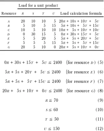
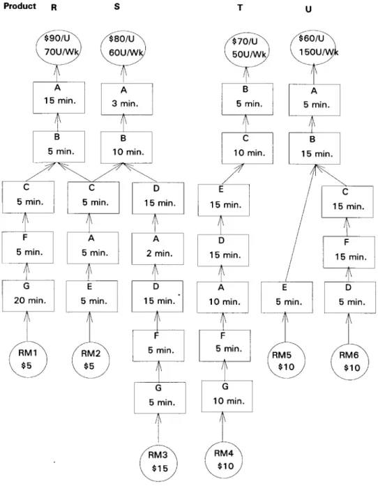
The example of Figure 1 ( modi® ed from Plenert 1993) attempts to show again how the TOC approach was considered to be incomplete for solving the product mix problem in a multiple-constraint case. Four product types, R , S , T and U are produced in seven dierent resources, A ± G , each of which has 2400 min capacity available. The load on each resource for producing one unit of product R , S , T and U can be collected to gen-erate the load calculation formula as shown in Table 1. The LP model is then formulated accordingly.
maximize 80R + 60S + 50t + 30U (1)
subject to
20R + 10S + 10T + 5U % 2400 ( for resource A) (2)
5R + 10S + 5T + 15U % 2400 ( for resource B) (3)
10R + 5S + 10T + 10U % 2400 ( for resource C) (4)
0R + 30S + 15T + 5U % 2400 ( for resource D) (5)
5R + 5S + 20T + 5U % 2400 ( for resource E) (6)
5R + 5S + 5T + 15U % 2400 ( for resource F) (7)
20R + 5S + 10T + 0U % 2400 ( for resource G) (8)
R% 70 (9)
S% 60 (10)
T % 50 (11)
U % 150 (12)
The following is the procedure of solving this problem using TOC.
S tep 1. Identify the system’s constraint( s)
The overload of each resource is computed, based on the market potential ( Table 2) . This reveals that resource B is the capacity constraint resource ( CCR) ( it is the most overloaded) .
S tep 2. D ecide how to exploit the system’s constraint( s) We calculate the $/constraint-minute for products
R , S , T and U to be 16, 6, 10 and 2, respectively ( Table 3) . Thus, according to the values of $/con-straint-minute, the order for manufacturing pref-erence is R , T , S and ® nally U . This results in the product mix solution 70R , 60S , 50T and 80U . The procedure is stopped and this solution is also the ® nal solution using the TOC approach, according to the description in previous papers. More detail of the TOC procedure can be found in Plenert ( 1993) .
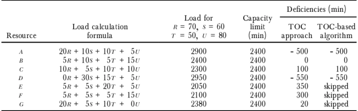
However, the above solution is infeasible. If we go further to calculate the load for each resource according to this solution, a capacity overload situation still exists ( as shown in Table 4) . That is, resources A and D are still overloaded. Comparatively, the solution derived by using a simplex method is, R = 50.67, S = 38.17, T = 50, and
U = 101. The throughput is 11 873.3.
Table 1. Load calculation formula for each resource. Load for a unit product
Resource R S T U Load calculation formula A 20 10 10 5 20R + 10S + 10T + 5U B 5 10 5 15 5R + 10S + 5T + 15U C 10 5 10 10 10R + 5S + 10T + 10U D 0 30 15 5 0R + 30S + 15T + 5U E 5 5 20 5 5R + 5S + 20T + 5U F 5 5 5 15 5R + 5S + 5T + 15U G 20 5 10 0 20R + 5S + 10T + 0U
Figure 1. Data for product mix example problem. Table 2. Capacity overloads for 70R , 60S , 50T and 150U .
De® ciencies ( min) Resource Load calculationformula
Load for R =70
,
S = 60 T = 50,
U = 150Capacity limit
( min) approachTOC TOC-basedalgorithm
A 20R + 10S + 10T + 5U 3250 2400
-
850-
850 B 5R + 10S + 5T + 15U 3450 2400-
1050-
1050 C 10R + 5S + 10T + 10U 3000 2400-
600-
600 D 0R + 30S + 15T + 5U 3300 2400-
900-
900 E 5R + 5S + 20T + 5U 2400 2400 0 skipped F 5R + 5S + 5T + 15U 3150 2400-
750 skipped G 20R + 5S + 10T + 0U 2380 2400 20 skippedThe remaining sections are organized as follows. The next section describes the basic work for exploiting all CCR( s) . This includes the categories of non-CCR( s) , the assumption of real value domain, and the way of fully utilizing all CCR( s) . Section 4 presents the algo-rithm. The above example will be solved again in the following section for further illustration. Finally, Section 6 draws conclusions.
3. Basic work for exploiting all CCR(s)
3.1. Categoriz ing non- CCR ( s)
A resource is an internal constraint if and only if the output of the resource is less than the market demand ( Fogarty et al. 1991) . A production system may face the single-constraint situation, in which only one resource is overloaded according to the market potential. In this situation, the CCR does not alter no matter what the product mix decision is. On the other hand, if a plant faces a multiple constraints situation, the CCR( s) may change as the product mix decision is changed. When solving the product mix problem, a single-constraint case is much easier to handle than a multiple-constraint case. In the multiple-constraints case, non-CCRs can be divided into three groupsÐ ® rst-level non-CCR( s) , sec-ond-level non-CCR( s) and the third-level non-CCR( s) .
First, second and third are named according to the order of ® nding them. Figure 2 shows the relationship.
A non-CCR( s) is said to be a ® rst-level non-CCR( s) when this resource is dominated by any other resource without considering what the product mix solution is. `A is dominated by B’ is de® ned as: for every product type the unit processing time required for B is always larger than that for A under the same level of capacity limit. Since this resource does not have the chance to have more load than any other resource, it is always non-CCR, unless the routeing of a product is changed.
The second-level non-CCR( s) is derived when we ® nd that its load calculated according to the market potential is lower than its capacity limit. This kind of non-CCR is also always ® xed. One additional reason to change the resource type is the change of market potential.
When the ® nal product mix solution is derived, a resource which is found to be underloaded is called a third-level non-CCR. In this situation, dierent product mix solutions ( product type and its corresponding quan-tity) yield dierent third-level non-CCR( s) .
When solving the product mix problem for one plan-ning period, the ® rst and second-level non-CCR( s) are ® xed and easily identi® ed. They can be neglected to simplify the problem. Identi® cation of the third-level non-CCR( s) becomes our focus for solving the product mix problem.
3.2. T he real- valued product mix solution
One assumption needed for this problem is that the solution of product mix decision is real-valued: this assumption we considered to be reasonable. The expla-nation is as follows: the product mix solution can be viewed as the production plan or target in a planning horizon. The remaining work in this planning horizon can be planned and implemented in the next horizon. Nevertheless, many factors will make the actual result deviate from the product mix plan. Factors include
inter-Table 3. Computing the pro® t contribution per constraint B minute.
Product
Parameter R S T U
Selling price ( $) 90 80 70 60 Raw material cost ( $) 10 20 20 30
Contribution ( $) 80 60 50 30
Constraint time ( resource B ) 5 10 5 15
$/constraint-minute 16 6 10 2
Table 4. Capacity overloads for 70R , 60S , 50T and 80U .
De® ciencies ( min) Resource Load calculationformula
Load for R = 70
,
S =60 T =50,
U = 80Capacity limit
( min) approachTOC TOC-basedalgorithm
A 20R + 10S + 10T + 5U 2900 2400
-
500-
500 B 5R + 10S + 5T + 15U 2400 2400 0 0 C 10R + 5S + 10T + 10U 2300 2400 100 100 D 0R + 30S + 15T + 5U 2950 2400-
550-
550 E 5R + 5S + 20T + 5U 2050 2400 350 skipped F 5R + 5S + 5T + 15U 2100 2400 300 skipped G 20R + 5S + 10T + 0U 2380 2400 20 skippedactions between process plans, ine cient scheduling, absence of materials, breakdown of resources, tool failure, and so forth. The next new plan for a time horizon will be made at the end of every scheduling period by using the rolling schedule concept. It seems unnecessary to limit the product mix solution to be integer.
3.3. Identifying and fully utiliz ing all CCR ( s)
The TOC approach is based on the CCR to give prod-ucts an order of manufacturing preference. It was con-sidered that it derived only the ® rst CCR and made other constraint resources untreated in a multiple-constraints situation. The iterative process included in the TOC ® ve steps was applied only when the constraints were broken ( in step 4) . However, the iteration process is still necessary for exploiting the constraints ( in step 2) .
Thus, one thing that should be explicit in the TOC approach is clari® cation of the iteration process. For each iteration, we have to identify the new CCR. The way to identify the next CCR is to choose the resource with the most capacity overload calculated according to the cur-rent product mix solution ( conforming to the concept of TOC) .
Once a new CCR is identi® ed, we have to decrease the quantity of the product type with the lowest priority to
eliminate the overload. The priority order is derived according to the `$/constraint-time’ value for each prod-uct ( still conforming to the concept of TOC) . However, there is a key problem: How do we give the values of the `S’ ( contribution) and the `constraint-time’ in each itera-tion? The analysis is depicted below. For convenience, the following notations are de® ned.
n the iteration number,
C C Rn the nth constraint identi® ed by the nth iteration,
Pn the quantity-adjustable product type identi® ed in the nth iteration for balancing the load of CCRn First, the formulation of the product mix decision pro-blem is given as follows.
maximize z =
å
n j=1 cjxj (13) subject toå
j=n1 aijxj% bi i = 1,
2,
. . .,
m (14) 0% xj% uj j = 1,
2,
. . .,
n (15) where cj is given as the contribution of product type j; aij denotes the time unit required for resource i to produce a type j product; xj ( bounded by the amount uj) is the Figure 2. Relationship among non-CCR( s) and CCR( s) .decision variable which represents the quantity of the product type j; bi represents the capacity limit of re-source i.
Suppose that resource r is the ® rst CCR, and there exists the next CCRÐ resource s. The following fact is observed to update the new values of the contribution margin `$’ and the `constraint time’ for a product type.
F act 1. Suppose that in the ® rst iteration, resource r has been the CCR and product u has been the chosen product ( it had the least value of `$/resource-r-time’ among all products) . Thus, the quantity of product u has been cut down to be equal to its upper capacity bound. In the second iteration, resources s are recognized as the second CCR. For any product denoted product j, if it is chosen to be cut down in quantity, then, cutting down one unit of product j will reduce
( 1) the load of resource s by (asj
-
asu*
arj/aru); ( 2) the contribution of the objective equation by(cj
-
cu*
arj/aru).( An explanation is given in the Appendix.)
From the fact, the `$/constraint-time’ for any product
j is
cj
-
cu*
arj/aru(
)
/(
asj-
asu*
arj/aru)
There arises another key problem. Once the quantity
Pn is changed in the nth iteration, all previous CCR( s) will lose the balance between load and capacity limit. Thus, to return all CCR equations to be `equality’ equa-tions again in the current ( nth) iteration, the quantities of the chosen products ( which are derived in previous itera-tions) must be adjusted. That is, if the load of CCRi(i
<
n) becomes over ( under) its capacity limit, then it should be decreased ( increased) by reducing ( increasing) the quan-tity of product Pi.On the basis of the preceding description and concept, the explicit TOC algorithm is developed.
4. The TOC-based algorithm for product mix determination
Two lemmas, discussed in Section 3.1 are utilized to reduce the complexity of the given problem.
L emma 1. Dominance rule. In a product mix decision problem, the capacity constraint for two dierent types of resources i and k can be expressed as:
ai1x1+ ai2x2+
´´´
+ ainxn% b0 (16)ak1x1+ ak2x2+
´´´
+ ak nxn% b0 (17)Here x1
,
x2,
. . .,
xn are the decision variables representing the quantities of products 1,
2,
. . .,
n. ai1 is the timerequired to produce product 1 using resource i, while
ak1 is the time required to produce product 1 using
resource k. If ai1% ak1, ai2% ak2
,
. . .,
ain% ak n, then resource i which is dominated by resource k, is a non-CCR. Here, we classify it as the ® rst-level non-non-CCR.L emma 2. In a product mix decision problem, if we substitute the market potential values of x1
,
x2,
. . .,
xn into the resource constraint expressed as equation ( 16) or ( 17) , and the inequality still holds, then this resource is also a non-CCR in the planning period. It is classi® ed as a second-level non-CCR in this paper.The ® rst-level and second-level non-CCR( s) never become CCR( s) for a given market potential. When deciding the product mix, they can be neglected ® rst. Hence, the TOC-based algorithm is as follows.
Preparation step. Delete the ® rst-level and the second-level non-CCR( s) using Lemmas 1 and 2. The current product mix solution is the market potential of each product type. Set n = 1, and no previous CCRi and Pi exist (i
<
n).S tep 1. Identify the system’s constraint.
Calculate the load of each resource based on the current product mix solution. Then compare the load of each resource with its capacity limit. The resource with the highest overload amount is identi® ed as the CCRn. If no CCR exists, then stop, and the current solution is the ® nal solu-tion.
S tep 2. Decide how to exploit the system’s constraint.
S tep 2a. Treat the CC Rn resource constraint as an equal-ity equation. Delete previous Pi(i
<
n) terms from this equation by manipulating the row operations between CCRn and CCRi(i<
n) equa-tion.S tep 2b. Also make the objective equation to be the new one without the previous Pn-1 term. It also can
be done by substituting the value of Pn-1, which
is derived from the CCRn-1 equality equation,
into the previous objective equation.
S tep 2c. Calculate the `$/constraint-time’ for all product types that have positive coe cients in CCRn equality equation, according to the new objec-tive equation ( step 2b) and the new CCRn equal-ity equation ( step 2a) .
S tep 2d. Choose the Pn which has the smallest `$/con-straint-time’ value for CCRn. Reduce the quan-tity of Pnuntil the load of the CCRnjust equals its capacity limit.
S tep 2e. Starting from CCRn-1 through CCR1, adjust the
quantity of previous Pi ( i
<
n) to make the loadof CCRi ( which is changed after performing step 2d) equal to its capacity limit again. Then, the new product mix is derived. Let n = n + 1 and go to step 1.
5. Example and veri® cation
To provide a better understanding of the algorithm, the example discussed in Section 2 is used.
In the preparation step, we determine the ® rst and the second-level non-CCR( s) by using Lemmas 1 and 2, and then ignore them. We observe that the time required on resource F for every product is less than that on resource
B. That is, 5% 5, 5% 10, 5% 5 and 15% 15. Thus, resource F is dominated by resource B . Also, resource G is dominated by resource A , since 20% 20, 5% 10, 10% 10 and 0
£
5. Resources F and G are ® rst-level non-CCRs. We then substitute the market potential quantities into the left constraints of the LP model. The results show that the inequality condition still holds for resource E ( i.e. 5*
70 + 5*
60 + 20*
50 + 5*
150% 2400) . According to Lemma 2, resource E is a sec-ond-level non-CCR.
After deleting the LP constraints of resources F , G and
E, the LP formulation becomes:
maximize Z = 80R + 60S + 50T + 30U (1)
subject to
20R + 10S + 10T + 5U % 2400 ( for resource A) (2) 5R + 10S + 5T + 15U % 2400 ( for resource B) (3)
10R + 5S + 10T + 10U % 2400 ( for resource C) (4)
0R + 30S + 15T + 5U % 2400 ( for resource D) (5)
R% 70 (9)
S% 60 (10)
T % 50 (11)
U % 150 (12)
The current product mix solution now is the market potentialÐ R = 70, S = 60, T = 50 and U = 150. The ® rst iteration(n = 1) begins.
Iteration 1
S tep 1. Identify the system’s constraint
The product mix R = 70, S = 60, T = 50 and
U = 150 is substituted into each resource con-straint. This reveals that resources A, B, C and D are overloaded, as shown in Table 2. Among
them, resource B is identi® ed as CCR1, since it
has the most overload.
S tep 2. Decide how to exploit the system’s constraint.
S tep 2a. Treat the resource B constraint `5R + 10S + 5T + 15U % 2400’ as `5R + 10S + 5T + 15U = 2400’. Since no previous CCRi and Pi exist, no manipulation is needed.
S tep 2b. Set `Z = 80R + 60S + 50T + 30U ’ as the cur-rent objective equation. Since no previous Pi exists, no adjustment is applied.
S tep 2c. Calculate the `$/constraint-time’ for all prod-ucts. The result is the same as with the TOC approach ( shown in Table 3) .
S tep 2d. Identify the product type U as P1, since it has
the smallest $/constraint-time.
U then is cut from 150 units to 80 units to make the load of CCR1 ( resource B ) meet its capacity
limitÐ 2400 min.
S tep 2e. The current product mix solution is 70R , 60S , 50T and 80U . This is also the solution given by the TOC approach. Now, we proceed to the second iteration.
Iteration 2
S tep 1. Identify the system’s constraint.
When substituting 70R , 60S , 50T and 80U into the resource constraints of the LP model, the resource overloads are shown in Table 4. Resource D is identi® ed as CCR2.
S tep 2. Decide how to exploit the system’s constraint.
S tep 2a. Treat the resource D constraint 0R + 30S + 15T + 5U % 2400 as 0R + 30S + 15T + 5U = 2400. The equation has to exclude the U term ( the previous chosen product) . By manipulating the row operations between the following equa-tions, we delete the U term from the CCR2
equation:
(CCR1 equation) 5R + 10S + 5T + 15U = 2400 (18) (CCR2 equation) 0R + 30S + 15T + 5U = 2400 (19)
The updated CCR2 equality equation is: (
-
5/3)R +(80/3)S +(40/3)T = 1600 (20)S tep 2b. The original objective equation is Z = 80R + 60S + 50T + 30U . The equation also has to exclude the U term. By substituting the value of U (U = 160
-
(1/3)R-
(2/3)S-
(1/3)Twhich is derived in the ® rst iteration) into the objective equation. The updated objective equa-tion becomes:
Z =4800 + 70R + 40S + 40T (21)
S tep 2c. Calculate the `$/constraint-time’ for products R ,
S and T , based on the above updated objective equation ( 21) and the equality equation ( 20) . Table 5 shows the results.
S tep 2d. Product S is chosen as P2. S then has to be
reduced to 315/8, in order that the C CR2
equal-ity equation ( 20) holds.
S tep 2e. Since the quantity of product type S is changed, the quantity of product U has to be changed again. That is, the equality equation 5R + 10S + 5T + 15U = 2400 has to be kept. Thus, U becomes 375/4.
Currently, the product mix solution is R = 70,
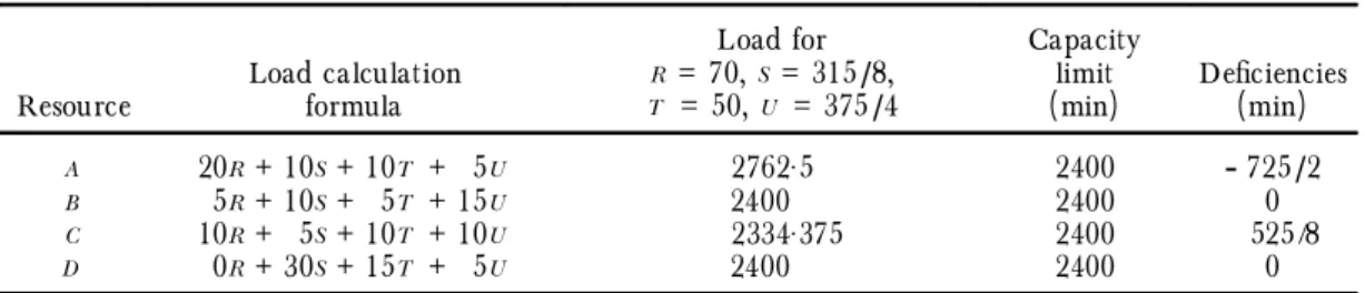
S =315/8, T = 50 and U = 375/4. Set n = 3 and con-tinue the third iteration.
Iteration 3
S tep 1. Identify the system’s constraint.
Table 6 shows the capacity overload/de® ciency situation based on the above product mix solu-tion. Now, resource A is the only one with over-loaded capacity in this iteration, and thus is
C C R3.
S tep 2. Decide how to exploit the system’s contraint.
S tep 2a. Treat 20R + 10S + 10T + 5U % 2400 ( for re-source A ) as CCR3 equality equation:
20R + 10S + 10T + 5U = 2400 (22)
Then, this equation, after excluding U and S terms, becomes: (75/4)R +5T = 1200. This is
derived by row operation between the following equations: ( CCR1equation) 5R + 10S + 5T + 15U = 2400 (18) (CCR2 equation)(
-
5/3R)+(80/3)S +(40/3)T = 1600 (20) (CCR3equation) 20R + 10S + 10T + 5U = 2400 (22)S tep 2b. CCR2 LP equation cannot be rewritten as
S =60 + (1/16)R
-
(1/2)T to represent the value of S . By substituting the S value into the previous objective equation Z = 4800 + 70R + 40S + 40T ( 21) , the current objective equation becomes Z = 7200 +(145/2)R +20T .S tep 2c. Calculate $/constraint-time for the remaining product types. Table 7 shows the results.
S tep 2d. Since 3.87 is smaller than 4, P3 is product type
R. R is the chosen product which has to be reduced. It becomes 50.67 ( 152/3) to force
C C R3 be an equality equationÐ (75/4)R +
5T = 1200.
S tep 2e. First, the quantity of product type S has to be adjusted to balance the CC R2 equality
equa-tionÐ (5/3)R +(80/3)S +(40/3)T = 1600. Hence, S becomes 229/6(38.17). Second, adjust the quantity of product U to keep the CCR1
equality equationÐ 20R + 10S + 10T + 5U = 2400. U becomes 101. Thus, the new product mix solution is R = 50.67, S = 38.17, T = 50 and U = 101.
Table 5. The pro® t contribution per constraint D minute. Product
Parameter R S T
Contribution ( $) 70 40 40
Constraint time ( resource D) ± 80/3 40/3
$/constraint-minute ± 3/2 3
Table 6. Capacity overload for 70R , ( 315/8) S , 50T and ( 375/4) U .
Resource Load calculationformula
Load for R = 70, S = 315/8, T =50, U = 375/4
Capacity limit
( min) De® ciencies( min)
A 20R + 10S + 10T + 5U 2762.5 2400
-
725/2B 5R + 10S + 5T + 15U 2400 2400 0
C 10R + 5S + 10T + 10U 2334.375 2400 525/8
D 0R + 30S + 15T + 5U 2400 2400 0
Table 7. The pro® t contribution per constraint A minute. Product
Parameter R T
Contribution ( $) 145/2 20
Constraint time ( resource A) 75/4 5
$/constraint-minute 3.87 4
The fourth iteration now begins. However, there is no
C C R4 found in step 1 ( see Table 8) . This means that the
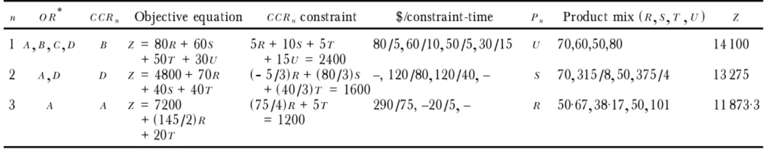
current product mix solution is the ® nal solution. We summarize the execution process of this algorithm in Table 9.
The dual-simplex method with bounded variables is very similar to our algorithm. Therefore, we use this method to test the eectiveness of our algorithm using the same example. The results, shown in Table 10 where R
Â
= 70-
R, SÂ
= 60-
S, TÂ
= 50-
T andU
Â
= 150-
U, are equal to those derived using our algo-rithm. The algorithm and the dual-simplex method give the same product mix solution in iteration 1, 2 and 3 and the same ® nal throughput.Observing the contents of Table 9 and Table 10, it is veri® ed that the design idea of the TOC approach is correct. However, the TOC approach is implicit and was considered to act as the ® rst iteration of the presented algorithm.
6. Conclusions
The TOC method has been applied to the product mix problem in two areas. In one area it is used as input for scheduling ( Schragenheim 1991) , and is called drum± buer± rope scheduling ( DBR) . Other areas include
master production planning and marketing ( Goldratt 1990) . However, the TOC approach to this problem is so implicit that it was considered to be an incomplete approach. That is, it derives infeasible solutions when the plant is in a multiple constraint situation.
In this paper, we make the TOC approach explicit. This includes successive iterations for deriving all CCR( s) , a method to update the value of `$/constraint-time’ , and quantity adjustment for previously chosen products. The presented algorithm derives the same result at each iteration as the dual-simplex method with bounded variables.
Some models, such as the market prices determination model ( Eden and Ronen 1990) and the strategic master production scheduling ( SMPS) model ( Ronen and Rozen 1992) , have been developed only for the single-constraint situation. However, because the situation of multiple constraint in a plant may appear in practice, the behaviour of these models may be distorted. To make a more accurate decision, there are two aspects that should be studied in future research:
( 1) Modify current models to ® t the situation of mul-tiple constraints.
( 2) Transfer the multiple-constraint situation to the single-constraint situation, and prevent it return-ing to the original status. The original model can then be applied.
Table 8. Capacity overload for 50.67R , 38.17S , 50T and 101U .
Resource Load calculationformula
Load for R =50.67, S = 38.17,
T =50, U = 101
Capacity limit
( min) De® ciencies( min)
A 20R + 10S + 10T + 5U 2400 2400 0
B 5R + 10S + 5T + 15U 2400 2400 0
C 10R + 5S + 10T + 10U 2207.55 2400 192.45
D 0R + 30S + 15T + 5U 2400 2400 0
Table 9. Summary of results.
n O R* C C Rn Objective equation C C Rnconstraint $/constraint-time Pn Product mix(R
,
S,
T,
U) Z 1 A,
B,
C,
D B Z =80R + 60S + 50T + 30U 5R + 10S + 5T+ 15U = 2400 80/5,
60/10,
50/5,
30/15 U 70,60,50,80 14 100 2 A,
D D Z =4800 + 70R + 40S + 40T (-
5/3)R +(80/3)S +(40/3)T =1600± , 120/80,
120/40,
± S 70,
315/8,
50,
375/4 13 275 3 A A Z =7200 +(145/2)R + 20T (75/4)R +5T = 1200 290/75, ± 20/5,
± R 50.67,
38.17,
50,
101 11 873.3 *O R: Overload resource.References
Ed e n, Y.,and Ro ne n, B.,1990, Service organization costing: a synchronized manufacturing approach. I ndustrial M anage-m ent, 24± 26.
Fo g a r t y, D. W ., Bl a c k st o ne, J . H., and Ho ffma nn, T. R ., 1991, P roduction and Inventory M anagem ent ( South-Western, Cincinnati) .
Go l d r a t t, E . M ., 1990, T he H aystack Syndrome ( North River, New York) .
Lu e b b e, R., and Finc h, B., 1992, Theory of constraints and linear programming: a comparison. International J ournal of P roduction R esearch, 30, 1471± 1478.
Pa t t e r so n, M . C.,1992, The product-mix decision: a compar-ison of theory of constraints and labor-based management accounting. P roduction and Inventory M anagement J ournal,
33( 3) , 80± 85.
Pl e ne r t, G., 1993, Optimizing theory of constraints when multiple constrained resources exist. E uropean J ournal of O perational R esearch, 70, 126± 133.
Ro ne n, B., and Ro z e n, E., 1992, The missing link between manufacturing strategy and production planning. Inter-national J ournal of P roduction R esearch, 30, 2659± 2681. Ro ne n, B.,and St a r r, M . K .,1990, Syncronized
manufactur-ing as in OPT: from practice to theory. Computer I ndustry E ng ineering, 18, 585± 600.
Sc h r a ge nh e im, E., 1991, DISASTERT M scheduling software teaching material ( Goldratt Institute, USA) .
A ppendix: Explanation of Fact 1
For the ® rst CCR ( resource r) , based on the current product mix solution, the LP constraint of resource r must be an `equality’ equation. That is,
ar1x1+ ar2x2+. . .+ aruxu+. . .+ arnxn= br (A1) Table 10. Solution tableau using the dual-simplex method with bounded variables.
1* BV* Z R
Â
SÂ
TÂ
UÂ
S1 S2 S3 S4 S5 S6 S7 RH* 0 Z 1 80 60 50 30 0 0 0 0 0 0 0 16 200 S1 0-
20-
10-
10-
5 1 0 0 0 0 0 0-
850 S2 0-
5-
10-
5-
15 0 1 0 0 0 0 0-
1 050 S3 0-
10-
5-
10-
10 0 0 1 0 0 0 0-
600 S4 0 0-
30-
15-
5 0 0 0 1 0 0 0-
900 S5 0-
5-
5-
20-
5 0 0 0 0 1 0 0 0 S6 0-
5-
5-
5-
15 0 0 0 0 0 1 0-
750 S7 0-
20-
5-
10 0 0 0 0 0 0 0 1 20 1 Z 1 70 40 40 0 0 2 0 0 0 0 0 14 100 S1 0-
55/3-
20/3-
25/3 0 1-
1/3 0 0 0 0 0-
500 UÂ
0 1/3 2/3 1/3 1 0-
1/15 0 0 0 0 0 70 S3 0-
20/3 5/3-
20/3 0 0-
2/3 1 0 0 0 0 100 S4 0 5/3-
80/3-
40/3 0 0-
1/3 0 1 0 0 0-
550 S5 0-
10/3-
5/3-
55/3 0 0-
1/3 0 0 1 0 0 350 S6 0 0 5 0 0 0-
1 0 0 0 1 0 300 S7 0-
20-
5-
10 0 0 0 0 0 0 0 1 20 2 Z 1 145/2 0 20 0 0 3/2 0 3/2 0 0 0 13 275 S1 0-
75/4 0-
5 0 1-
1/4 0-
1/4 0 0 0-
725/2 UÂ
0 3/8 0 0 1 0-
3/40 0 1/40 0 0 0 225/4 S3 0-
105/16 0-
15/2 0 0-
11/16 1 1/16 0 0 0 525/8 SÂ
0-
1/16 1 1/2 0 0 1/80 0-
3/80 0 0 0 165/8 S5 0-
55/16 0-
35/2 0 0-
5/16 0-
1/16 1 0 0 3 075/8 S6 0 1/16 0-
5/2 0 0-
17/16 0 3/16 0 1 0 1575/8 S7 0-
325/16 0-
15/2 0 0 1/16 0-
3/16 0 0 1 985/8 3 Z 1 0 0 2/3 0 58/13 8/15 0 8/15 0 0 0 11 873.3 RÂ
0 1 0 4/15 0-
4/75 1/75 0 1/75 0 0 0 58/3 UÂ
0 0 0-
1/10 1 1/50-
2/25 0 1/50 0 0 0 49 S3 0 0 0-
11/2 0-
7/20-
3/5 1 3/20 0 0 0 385/2 SÂ
0 0 1 31/60 0-
1/300 13/600 0-
11/300 0 0 0 131/6 S5 0 0 0-
199/12 0-
11/60-
4/15 0-
1/60 1 0 0 2 705/6 S6 0 0 0-
151/60 0 1/300-
319/300 0 14/75 0 1 0 587/3 S7 0 0 0-
25/12 0-
13/12 1/3 0 1/12 0 0 1 3 095/6I*: iteration, BV*: basic variable, RH*: right-hand side.
To make the resource r fully utilized and the above equa-tion hold when xj reduces by one unit, xu needs to increase by arja/ruunit( s) .
For the second CCR ( resource s) , its current load is denoted by the left-hand side of its constraint
as1x1+ as2x2+
´´´
+ asuxu+´´´
+ asnxn. Since xj reduces by one unit and xu dependently increases by arj/aru unit( s) , this causes the load of resource s be reduced byasj
-
asu*
arj/aru.The substitution is also applied to the objective function (c1x1+ c2x2+
´´´
+ cuxu+´´´
+ cnxn). When xj reduces by one unit, xu dependently increases by arj/aru unit( s) . This causes the objective value ( contribution) to be reduced by cj-
cu*
arj/aruThe above result can also be derived by the following row operations using the Gaussian elimination method. The new objective equation without the xu term is
z
Â
= (c1-
ar1*
cu/aru)*
x1+(c2-
ar2*
cu/aru)*
x2+´´´
+(cu
-
aru*
cu/aru)*
xu+´´´
+(cn-
arn*
cu/aru)*
xn (A2)That is done in the same way as the previous objective equation
-
(cu/aru)*
equality equation of resource r.Similarly, by row operation the new resource s LP constraint without the xu term is its original constraint
-
asu/aru*
resource r equality equation. It becomes (as1-
ar1*
asu/aru)*
x1+ (as2-
ar2*
asu/aru)*
x2+´´´
+(asu
-
aru*
asu/aru)*
xu+´´´
+(asn
-
arn*
asu/aru)*
xn% bs-
br*
asu/aru (A3) Thus, `$/constraint-time’ for any product type j is(cj