WiMAX系統下兩階級數據的數據映射演算法之改進

國

立

交

通

大

學

電信工程研究所

碩 士 論 文

WiMAX 系統下兩階級數據的數據映射演算法之改進

An Enhanced Data Mapping Algorithm for Two-Level Requests

in WiMAX Systems

研 究 生：黎廷勇

指導教授：李程輝 教授

WiMAX 系統下兩階級數據的數據映射演算法之改進

An Enhanced Data Mapping Algorithm for Two-Level Requests

in WiMAX Systems

研 究 生：黎廷勇 Student：Dinh-Dung Le

指導教授：李程輝教授 Advisor：Prof. Tsern-Huei Lee

國 立 交 通 大 學

電信工程研究所

碩 士 論 文

A Thesis

Submitted to Institute of Communications Engineering College of Electrical Engineering and Computer Engineering

National Chiao Tung University in partial Fulfillment of the Requirements

for the Degree of Master

in

Communications Engineering

July 2013

Hsinchu, Taiwan, Republic of China

WiMAX 系統下兩階級數據的數據映射演算法之改進

研究生：黎廷勇 指導教授：

李程輝 教授

國立交通大學

電信工程研究所

摘要

IEEE 802.16e 標準，採用 OFDMA PHY 一般被稱為行動 WiMAX (Mobile WiMAX)， 在過去的幾年中已經引起了無線通信業界的關注。它是一個基於 IP 網路的高速遠 距離無線寬帶接取技術的優化。在行動 WiMAX 系統的下行鏈路，數據都被映射到 矩形區域。在矩形的限制下，最大化吞吐量是一個 NP 完全問題。過去有一些啟發 式數據映射算法被提出，他們試圖實現系統的高吞吐量。其中有大多數的演算法 只處理一種類型的數據。在最近的研究中，一個可映射兩級別的數據請求（即緊 急和非緊急數據）的數據映射演算法被提出。然而，它在決定數據映射的順序時 卻只有考慮數據請求所需的槽數量。 在這篇論文中，我們提出的增強版本，同時考慮每個行動用戶所需的槽數量 和所使用的調變編碼機制。模擬結果顯示，與以前的設計相比，增強的演算法能 為緊急數據提供更高的吞吐量。

An Enhanced Data Mapping Algorithm for

Two-Level Requests in WiMAX Systems

Student: Dinh-Dung Le Advisor: Prof. Tsern-Huei Lee

Institute of Communications Engineering,

National Chiao Tung University

Abstract

The IEEE 802.16e standard, which adopts OFDMA PHY and is generally known as Mobile WiMAX, has grabbed the attention of wireless communication industry for the past few years. It is a technology optimized for IP-based high speed long-distance wireless broadband access. In the downlink of Mobile WiMAX systems, data requests have to be mapped into rectangular regions. Such a constraint results in an NP-complete problem in order to maximize throughput. Several heuristic data mapping algorithms were proposed trying to achieve high system throughput. Most of the algorithms handle only one type of data. In a previous research, a data mapping algorithm which maps two levels of requests, i.e., urgent and non-urgent data, has been presented. However, only the number of required slots were considered in determining the order of data mapping.

In this thesis, we propose an enhanced version which considers both the number of required slots and the modulation level for each mobile station. Simulation results show that, compared with previous design, the enhanced algorithm serves more urgent data with higher throughput.

Acknowledgements

I would like to acknowledge my advisor, Prof. Tsern-Huei Lee, for his valuable guidance throughout my research. I would also like to express my appreciations to Prof. Yaw-Wen Kuo for his kind helps and useful suggestions. Next, I wish to thank all members in 823 Lab, especially Yang-Zi Yang and Tzu-Han Wu, for helping me through my academic years; they all played an important role during my studies here in Taiwan. Last but not least, I would like to thank my family for their encouragements and supports.

Contents

List of Figures ... vii

Chapter 1 Introduction ... 1

1.1 An Overview of WiMAX System ... 1

1.2 Downlink Burst Mapping Problem ... 3

1.3 Objective... 5

1.4 Thesis Organization ... 6

Chapter 2 Related Works ... 7

2.1 Enhanced OCSA (eOCSA) ... 7

2.2 Two-Level Requests Mapping (TLRM) ... 9

2.3 DL Data Mapping Examples using Related Algorithms ... 10

2.3.1 DL data mapping using eOCSA ... 11

2.3.2 DL data mapping using TLRM... 14

Chapter 3 Proposed Algorithm ... 18

3.1 System Model and Definition ... 18

3.2 E-TLRM Description... 19

3.2.1 E-TLRM first phase ... 19

3.2.2 E-TLRM second phase ... 21

Chapter 4 Performance Evaluation ... 27 Chapter 5 Conclusions ... 33 Bibliography ... 34

List of Tables

Table 2.1 The set of data requests using in related algorithm examples ... 10

Table 2.2 eOCSA example results... 13

Table 2.3 TLRM example results ... 16

Table 3.1 An example of proposed algorithm ... 23

Table 3.2 E-TLRM example results ... 26

List of Figures

Fig. 1.1 A simple OFDMA DL sub-frame structure. ... 2

Fig. 1.2 Resource wastage in DL Mapping. ... 5

Fig. 2.1 An example of mapping DL bursts using eOCSA. ... 8

Fig. 2.2 DL data mapping using eOCSA. ... 13

Fig. 2.3 The first phase of TLRM algorithm. ... 15

Fig. 2.4 The second phase of TLRM algorithm. ... 17

Fig. 3.1 Example of a general burst in DL sub-frame. ... 21

Fig. 3.2 An Example of DL data mapping using E-TLRM algorithm. ... 25

Fig. 4.1 Average unused slots vs. number of MSs. ... 29

Fig. 4.2 Average over allocated slots vs. number of MSs. ... 30

Fig. 4.3 Average efficiency vs. number of MSs. ... 31

Fig. 4.4 Average number of mapped MUST parts vs. number of MSs. ... 31

Chapter 1 Introduction

1.1

An Overview of WiMAX System

Mobile WiMAX based on the IEEE 802.16e standard [1] has been introduced as the first broadband wireless access technology that supports both fixed and mobile environments. The IEEE 802.16e standard specifies the physical (PHY) and Medium Access Control (MAC) layers while the WiMAX Forum ensures interoperability between different manufactures’ devices. In fact, there are three different PHY layers defined: Single-Carrier PHY, Orthogonal Frequency-Division Multiplexing (OFDM) PHY, and Orthogonal Frequency-Division Multiple Access (OFDMA) PHY. Compared to the other PHY technologies, the OFDMA PHY is superior and has therefore been selected by the WiMAX Forum because of its features such as reducing the granularity in the radio resource mechanism, using the available power more efficiently, and leading to a significant cell range extension in the uplink transmission [2].

In the IEEE 802.16e OFDMA system, while both Frequency Division Duplexing (FDD) and Time Division Duplexing (TDD) operation modes are specified, there are many initial products and deployment scenarios currently focusing on TDD operation because of the flexibility to partition downlink (DL) and uplink (UL) resources and better channel reciprocity to support closed enhancing techniques [3]. In the TDD system, the time domain is divided into 5ms frames, which are separated into DL and UL sub-frames [4].

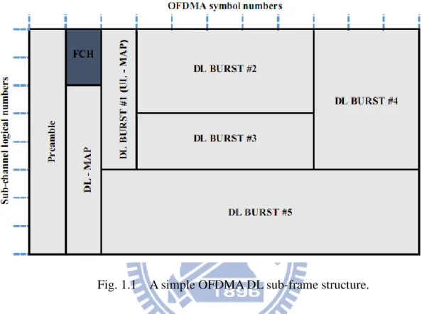
As can be seen in Fig. 1.1, an OFDMA DL sub-frame begins with a DL preamble which is used for frame synchronization, channel state estimation, received signal

strength, and signal-to-interference-plus-noise ratio (SINR) estimation; and followed by Frame Control Header (FCH), downlink map (DL-MAP) and uplink map (UL-MAP) messages that describe the structure and composition of frame.

Fig. 1.1 A simple OFDMA DL sub-frame structure.

According to the IEEE 802.16e specification, the units of resource allocation are slots, bursts and permutation zones. A slot is the minimum possible data allocation unit in time and frequency dimensions. It’s a combination of a sub-channel and one or more OFDMA symbols depending on sub-carrier permutation mode. On the downlink, a burst denotes a rectangular region which consists of a group of contiguous logical sub-channels in a group of contiguous OFDMA symbols. Each burst is transmitted using a single Modulation and Coding Scheme (MCS) and may include MAC protocol data units (PDUs) intended for one or more users. A permutation zone denotes an allocation in time when one particular subcarrier permutation mode is used to map data symbols onto sub-channels. A downlink sub-frame may contain more than one

permutation zone.

In this thesis, we only consider the downlink sub-frame with Partially Used Sub-Channelization (PUSC) zone wherein the sub-carriers are fairly distributed over the entire frequency band by using PUSC permutation mode. With PUSC mode, a slot will be a combination of one sub-channel and two OFDMA symbols; according to WiMAX Forum specified parameters, with 10 Mhz spectrum, there are 30 sub-channels, each one consists of 28 sub-carriers.

The IEEE 802.16e standard has defined 5 scheduling service classes with different QoS requirements, including bandwidth, packet loss, delay, and delay jitter: Unsolicited Grand Service (UGS), real-time Polling Service (rtPS), extended real-time Polling Service (ertPS), non-real-time Polling Service (nrtPS), and Best Effort (BE) [5][6]; each class has different QoS parameters.

Moreover, the standard also specifies that each data burst has to be mapped into a rectangular region of the downlink sub-frame. This constraint makes the DL mapping as two-dimensional downlink burst mapping problem introduced in the next section.

1.2

Downlink Burst Mapping Problem

The two-dimensional downlink burst mapping problem in Mobile WiMAX system is a variation of the bin packing problem, which is known to be NP-complete [7].

In order to define the problem, assume that the DL sub-frame is a two-dimensional matrix of slots, and the area of each burst is expressed in term of slots. Let c and s

be the number of sub-channels and number of time slots in a DL sub-frame, respectively. Thus the total resource in a frame is B s c slots. Given a set of n items

1 2

{ ,b b ,..., }b , and each item _n b has a size _i A , 1 i_i  n. All items are mapped into B

under the following constraints:

 No overlap between any two rectangular bursts regions.

 A_i W_iH_i. Where W and _i H are the width and the height of the _i

rectangle burst assigned to item ith, respectively.

 W_i s and H_i c for all i.

However, the OFDMA downlink burst mapping is different from the typical bin packing. First, the dimensions of rectangles are predetermined in the bin packing, while the bursts can be sharped flexibly. Second, there can be resource wastage due to the size mismatch between the data requests and the allocated burst, which does not exist in the bin packing. When the actual data belonging to a request cannot fill the whole rectangular region of a burst, the vacant slots are considered as over allocated slot wastage within the burst. Besides, in some cases the remaining slots in the DL sub-frame cannot form a rectangle to fit any unmapped requests. These remaining slots are called unused slot wastage outside the bursts. Both these wasted slots reduce the efficiency and should be minimized. Fig. 1.2 is an example about resource wastage in DL Mapping.

For this example, over allocated slots and unused slots are shown in black and white, respectively.

Fig. 1.2 Resource wastage in DL Mapping.

1.3

Objective

The problem of efficiently mapping the DL data requests into rectangular regions in the DL sub-frame as mentioned above is not addressed by the IEEE 802.16e standard, and is left as an implementation issue. As a result, several DL mapping algorithms have been proposed in literature recently [8]-[11]. In particular, a mapping algorithm which handles two levels of data requests, i.e., urgent and non-urgent data, was presented in [12]. For convenience, we shall refer to this algorithm Two-Level Requests Mapping (TLRM).

In TLRM algorithm, each user’s request can consist of urgent and non-urgent data. The algorithm consists of two phases. Phase 1 maps all requests with both urgent and non-urgent parts into the DL sub-frame, and Phase 2 returns some mapped non-urgent data parts so that more urgent data parts can then be mapped. The goal of TLRM algorithm is to map the real-time traffic effectively but do not focus on the urgent part in the first phase. Moreover, if several MCSs are used, the mapping order based on the required number of slots becomes inefficiency. Suppose that there are two requests with

the same size. The one with a worse MCS is mapped prior to the other which may be unmapped when there are no enough slots for both, resulting in a low spectrum efficiency.

The purpose of this thesis is to present an enhanced version of the TLRM algorithm. In addition to the number of required slots, we also consider achievable Modulation and Coding Scheme (MCS) of urgent data in determining the order of data mapping. Simulation results show that, compared with previous design, the enhanced algorithm serves more urgent data with higher throughput. Simulation results show that, compared with previous design, the enhanced algorithm serves more urgent data with higher throughput.

1.4

Thesis Organization

The rest of this thesis is organized as follows. In Chapter 2, the related algorithms eOCSA and TLRM will be reviewed in detail. Our proposed data mapping algorithm, called Enhanced Two-Level Requests Mapping (E-TLRM) in WiMAX Systems, is briefly introduced and described in Chapter 3. Details of the performance evaluation of our E-TLRM algorithm when compared with eOCSA and TLRM are given in Chapter 4. Finally, Chapter 5 gives our conclusions.

Chapter 2 Related Works

This chapter presents a comprehensive introduction to related DL mapping algorithms, including the eOCSA and TLRM algorithms. eOCSA [14] is the enhanced version of One Column Stripping with non-increasing Area first mapping (OCSA) [13], aims to keep the mapping operational complexity low. Based on the eOCSA algorithm, TLRM is introduced to effectively map the sensitive real-time traffic.

2.1

Enhanced OCSA (eOCSA)

In eOCSA, the data requests are sorted in the descending order (largest first) and are mapped into the DL sub-frame from bottom to top and from right to left to allow the space for variable portions of the DL-MAP.

Let H denote the maximum height in the DL sub-frame and A =

 

1

N i i

A _ denote the set of N data requests. The eOCSA scheme consists of four steps. In the first step, the algorithm sorts the set of data requests in the descending order and selects the largest request, say, A . In the second step, also known as vertical mapping, eOCSA _k

maps the request A to a rectangle with width W_{k k} and height H . _k

W_k  _A_k/H_ (1)

/ W

k k k

H  _A _ (2)

Where,  _{ } denotes the ceiling function, which is ensures that the mapped region is bigger than required data request (W_kH_k A_k) and has the minimum possible width (minimizing MS active time and energy).

The remaining unallocated space is handled in the third step, during which the

horizontal mapping takes place as the algorithm looks for the next largest data request

that will fit into the space left on the top of the burst mapped in the previous step. But here, the widths of all following bursts mapped in the strip are fixed to that of the burst mapped in the previous step. In other words, the height of each burst allocated in the strip is calculated as the ceiling function of the data request divided by the fixed width. This process is repeated until no space can be allocated or there is no data request that can fit in this space. Next, the algorithm moves leftward to fill the remaining empty columns in the DL sub-frame and repeats the process from the second step.

Fig. 2.1 An example of mapping DL bursts using eOCSA.

Fig. 2.1 shows the process of moving vertically and horizontally from bottom to top and right to left. Note that when the data request is smaller than the mapped region,

2.2

Two-Level Requests Mapping (TLRM)

In fact, a data request can consist of two parts (or two levels): MUST part and WISH part. The MUST part is the urgent data which will be dropped if it is not mapped anđ the WISH part represents non-urgent data that can be transmitted in later frames. For instance, rtPS, UGS, and ertVR regarded as urgent data called MUST data; while nrtPS and BE are treated as non-urgent data called WISH data.

TLRM algorithm is divided into two phases. In the first phase, TLRM basically uses a modified version of eOCSA algorithm, with two-level requests. However, for two-level requests, the scheme requires that when mapping the data requests into rectangles, the MUST part is allocated first, followed by the MUST part. The first phase can be separated into 4 steps. In the first step, the algorithm selects a strip which is a group of contiguous columns in the DL sub-frame. The strip has the width W and an largest empty space called maximum available rectangle space, say Ri,j. In the second step, the TLRM selects the largest two-level request Ak in the set of data requests such that Ak can be mapped into the Ri,j found in the previous step. The first phase terminates if no such Ak exists. In the third step, the algorithm maps Ak into Ri,j. If there is no mapped request in the strip, the algorithm maps Ak to a rectangle with width W* and height H*, where W*= Ak/Hand H*= Ak/H. Here, if W* is smaller than W, the algorithm divides the selected strip into 2 smaller strips of widths W* and W- W*. In case some requests had been mapped in the selected strip, the algorithm maps Ak to a rectangle with width W and height H*_{, where H}*= Ak/W. Next, the algorithm updates the maximum available rectangle spaces in the strips and removes Ak from the set of data requests.

After the first phase is completed, usually there are some remaining requests that were not mapped. Since these “unmapped requests” might contain the MUST part and WISH part, the second phase consist of mapping as much MUST part as possible for those unmapped requests. Firstly, the algorithm selects the unmapped request Ak whose MUST part Mk is the largest one. Secondly, it selects a proper strip to map Mk. If Mk is less than the maximum available rectangle space Ri,j for some strips, the strip with the smallest Ri,j will be selected. Otherwise, the algorithm selects strip with largest over allocated slots and removes some WISH data of the mapped requests, so that Mk can fit in the strip. Thirdly, Mk is mapped into the selected strip same as the third step of the first phase. If there are unused slots in the strip, the scheme continues to map WISH part of Ak. Finally, Ak is removed from the set of data requests.

2.3

DL Data Mapping Examples using Related Algorithms

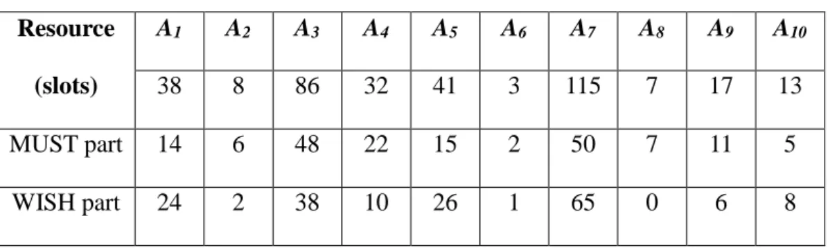
In this section, we provide 2 examples that help explain the operation of eOCSA and TLRM algorithms. Assume that there are 12 timeslots and 30 sub-channels in the DL sub-frame. There are 10 MSs with the data request set A as show in Table 2.1. The sum of all data requests is 360, in which the sum of the MUST part of all requests is equal to 180.

Table 2.1 The set of data requests using in related algorithm examples Resource (slots) A1 A2 A3 A4 A5 A6 A7 A8 A9 A10 38 8 86 32 41 3 115 7 17 13 MUST part 14 6 48 22 15 2 50 7 11 5 WISH part 24 2 38 10 26 1 65 0 6 8

2.3.1 DL data mapping using eOCSA

First, eOCSA sorts all the data requests shown in Table 2.1 in the descending

order of the request size and selects the largest request to map first (step 1). After finished step 1, the order of set A is { A7; A3; A5; A1; A4; A9; A10; A2; A8; A6 } and the largest data request A7 = 115 is chosen to map first.

Appling step 2, we get a width of _115 / 30_4 columns and a height of

115 / 4 29

 

  rows. The rectangle 4 29 results in an over allocated of 1 slot. The downlink sub-frame mapping is done from right to left and from bottom to top. The mapping of A7 into the sub-frame leaves a strip of 4 1 .

In step 3, the algorithm chooses the next largest data request that can fit into the

remaining strip, which is A6 = 3. And it is mapped as 4 3 / 4 or 4 1 , resulting in 1 over allocated slot. Since there is no left-over space within this strip, we repeat step 2 by moving horizontally to the left.

The next largest data request is A3 = 86, mapped into the DL sub-frame in a rectangle of width _85 / 30_3 and height _85 / 3_29. The rectangle mapping of 3 29 results in an over allocated of 1 slot and a left-over strip of 3 1 on the top. Since there is no data request that can be fitted into the remaining space, eOCSA repeats step 2 by moving horizontally to the left.

The next largest data request is A5 = 41, mapped into the DL sub-frame in a rectangle of width _41 / 30_2 and height _41 / 2_21. The rectangle mapping of

2 21 results in an over allocated of 1 slot and a left-over strip of 2 9 on the top. The algorithm then moves to step 3 to fill the 2 9 strip. The next largest data request that can fit into this strip is A9 = 17, which is mapped to a rectangle 2 17 / 2 or 2 9 , resulting in 1 over allocated slot and no left-over space on the top. Since there is no left-over space within this strip, we repeat step 2 by moving horizontally to the left.

At this time, the largest request in set A is A1 = 38, which is mapped to a rectangle of 2 19 , with no over allocated slot and a 2 11 left-over space. The scheme moves again to step 3 to look for the largest request that can fit into the remaining space 2 11 .

A10 = 13 being mapped to a rectangle of 2 13 / 2 or 2 7 ; resulting in 1 over allocated slot and a left-over space of 2 4 on the top. Then A2 = 8 being mapped to a rectangle of 2 _8 / 2_ or 2 4 ; resulting in no over allocated slot and no left-over space of on the top. eOCSA continues to repeat step 2 by moving horizontally to the left.

The next largest request A4 = 32 cannot fit in the remaining space of DL sub-frame, so the request A8 = 7 being mapped to a rectangle of 1 7 / 1 or 1 7 ; with no over allocated and a 1 23 left-over on the top. Unfortunately, there are no requests that can fit into this left-over space, so the algorithm is terminated.

In this example, the over allocated slots are 1 1 1 1 1 1 6      , and the total unused slots is 3 1 1 23 26    ; the efficiency of the algorithm (percented of used space) is 91.11%, with over allocated and unused slots being counted as wasted space. The final results of this example are shown as Table 2.2.

Table 2.2 eOCSA example results

Over allocated Slots 6

Unused Slots 26

Unmapped data requests 1

Efficiency 91.11%

The DL data mapping results of this example is shown in Fig. 2.2. Where the dark represent the over allocated slots, and the white represent the unused slots; areas in gray are all the mapped data requests.

2.3.2 DL data mapping using TLRM

In this example, assume that each data request consists of two parts: MUST part and WISH part, which are shown as Table 2.1.

 First Phase:

This phase tries to map both MUST and WISH parts of a data request into the DL sub-frame.

In the first iteration, TLRM selects strip K1,12, which has the width W_1,12 12 and the maximum available rectangle 12 30 , and selects the largest request smaller than 12 30 360 is A7 = 115 (step 1, 2). According to step 3, we get a width of

115 / 30 4

 

  columns and a height of _115 / 4_29 rows. The data request A7 is mapped into the rectangle 4 29 with 1 over allocated slot. The downlink sub-frame mapping is done from right to left and from bottom to top. Since the width of rectangle 4 29 is smaller than the width W1,12, strip K1,12 is split into K1,4 and K5,12 . The widths

and maximum available rectangles of K1,4 and K5,12 are W1,4 4,4 1 and W5,128,

8 30 , respectively.

In the second iteration, the maximum available rectangle 8 30 of K5,12 and the next largest data request A3 = 86 are selected. According to step 3, we get a width of

86 / 30 3

 

  columns and a height of _86 / 3_29 rows. The data request A7 is mapped into the rectangle 3 29 with 1 over allocated slot. The downlink sub-frame mapping is done from right to left and from bottom to top. Since the width of rectangle 3 29 is smaller than the width W_5,12, strip K5,12 is split into K5,7 and K8,12 . The widths

and maximum available rectangles of K5,7 and K8,12 are W5,73,3 1 and W8,125,

5 30 , respectively.

Similarly, the next largest data request is A5 = 41, mapped into the DL sub-frame in a rectangle of width _41 / 30_2 and height _41 / 2_21in the third iteration. The rectangle mapping of 2 21 results in an over allocated of 1 slot and strip K8,12 is split into K8,9 and K10,12.

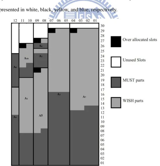
The first phase is executed for six more iterations to senquentially map the data requests A1, A9, A10, A2, A8 and A6. Fig. 2.3 shows the DL data mapping results of the first phase. Where the unused slots, over allocated slots, MUST parts, and WISH parts are presented in white, black, yellow, and blue, respectively.

 Second Phase:

After finishing the first phase, we have 5 strips in the DL sub-frame: K1,4, K5,7, K8,9,

K10,11, K12,12 and its maximum available rectangles are 4 1 4  , 3 1 3  , 2 3 6  , 2 4 8  , 1 6 6, respectively. The algorithm will try to map the MUST part M4 = 22 of the unmapped request A4 = 32 in the second phase.

According to step 2, TLRM chooses the strip K8,9 with the largest value of over allocated slots (2) to fit M4. Since the number of unused slots in K8,9 is 6 slots, the algorithm will remove 14 slots belonging to the WISH parts of A6, A2, and A5. Then, M4 being mapped to the rectangle of 2 11 in the top of K8,9. Finally, the algorithm is terminated. The DL data mapping results of the second phase is shown in Fig. 2.4.

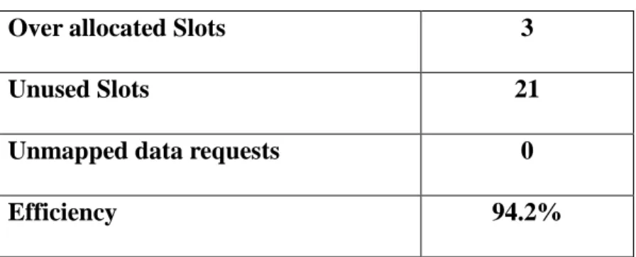
In this example, the over allocated slots are 1 1 1 3   , and the total unused slots is 4 1 3 1 2 4 1 6       21; the efficiency of the algorithm (percentage of used space) is 94.2%, with over allocated and unused slots being counted as wasted space. The final results of this example are shown as Table 2.3.

Table 2.3 TLRM example results

Over allocated Slots 3

Unused Slots 21

Unmapped data requests 0

Fig. 2.4 The second phase of TLRM algorithm.

Chapter 3 Proposed Algorithm

In general, Mobile WiMAX supports a variety of modulation and coding schemes (MCSs) to adapt and adjust the transmission based on channel conditions. As a result, a data request may require different burst sizes if different MSCs are used. In order to meet QoS requirements and maximize system throughput, larger urgent data with higher MCS should have higher mapping priority. This chapter describes our data mapping algorithm called Enhanced Two-Level Requests Mapping (E-TLRM), which considers both the size and available MCS of urgent data.

3.1

System Model and Definition

In this thesis, we adopt a WiMAX system which consists of a Base Station (BS) and N Mobile Stations (MSs). Each MS has a data request for the DL transmission.

Let represent the set of MSs where N denotes the number of MSs. Let i

r denote the data request of user i which consists of urgent data, r_iM and non-urgent data, W

i

r , i.e., M W

i i i

r r r , 1 i  N

We only consider the downlink sub-frame with Partially Used Sub-Channelization (PUSC) zone wherein the sub-carriers are fairly distributed over the entire frequency band by using PUSC permutation mode. With PUSC mode, a slot will be a combination of one sub-channel and two OFDMA symbols.

In this system, several MCSs can be used to adapt the transmission rate to the channel conditions. Assume that the set of MCSs from the lowest to highest which are

level from 1 to L. Based on the link quality, the BS decides a MCS level for each data request. Let mi denote the MCS level that BS uses for the data request r , 1_i m_i L and

i

m

 is the number of bytes which a slot can carry with the MCS level m . _i

Let A denote the set of requests for mapping A ={ }A_{i i}N(in number of slots). A request A will be the sum of two parts: the MUST part, _i M , and the WISH part, _i W_i, i.e.,A_i M_iW_i, where / i M i i m M  r  _and W W / i i  ri m1 i  N

Assume that there are s timeslots and c sub-channels in the DL sub-frame. Let

Ω ={( , )|1x y  x s,1 y c} be the set of all slots in the sub-frame. Let K_{i j,} be a vertical strip which consists of columns i to j , 1 i  j s. A rectangle R is denoted by





width, and the height, respectively. Also, denote R as the area of R. Let the rectangle Ri j, be the maximum available rectangle in Ki j, .

3.2

E-TLRM Description

E-TLRM, similar to TLRM, is divided into two phases. The first phase consists of mapping all two-level requests with both MUST parts and WISH parts in descending order of MCS level and MUST part’s size into the DL sub-frame. The second phase consists of returning some mapped requests’ WISH parts, so that more MUST parts of unmapped requests can be mapped.

3.2.1 E-TLRM first phase

The first phase consists of four steps. The proposed algorithm maps slots to a request iteratively. Let be the set of all strips, and initially ={K_1,s}.

 Step 1: Sort the set of requests A in the descending order of MCS level m . Two _i

requests using the same MCS level are sorted according to MUST part’s size M . _i

Requests with the same MCS level and MUST part’s size are sorted based on the sizes of their WISH parts. Ties are broken arbitrarily. For convenience, the set of sorted requests is called sorted_A whose elements are mapped sequentially. Consequently, requests with higher MCS levels have higher priority. The first phase terminates after the last element in sorted_A is handled.

 Step 2: Let A be the request to be mapped. Select the first strip in _k say

*_, *

i j

K , which can accommodate A in its maximum available rectangle _k R_i*_{, j}* . K_i*_,j*

and R_i*_{, j}* are denoted by

* * *

( ,1); (i j i 1),c

   

  and _{( ,i}* _y'_{); (j}* _i* _1),h'

  ,

respectively. In case that no such strip exists, we proceed to next request with the same operation.

 Step 3:Map A_k to R_i*_{, j}*. There are two cases for K_i*_{, j}*:

i) If K_i*_,j*  R_i*_,j* , there is no requests mapped in K_i*_{, j}* and K_i*_{, j}* must be *_,

i s

K .

a. Calculate w _A_k/c_ and h _A_k/w_. Allocate the rectangle

*

( ,1); ,

R  i w h_ for request A . _k

b. If ws i- *1, then split the strip K_i*_{, j}* into K_{i i}*_,*_w-1 and K_i*_{w s,} .

ii) Otherwise there are some requests mapped in K_i*_{, j}*. Calculate * * w j  i 1 and h Ak/w. Allocate * ' ( , ); , R  i y w h_ for request A_k.

 Step 4: Update R_i*_{, j}* or (R_{i i}*_,*_w-1and R_i*_{w s,} ). Remove A_k from sorted_A.

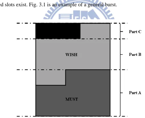
In general, a burst in the DL subframe may consist of up to three contiguous parts. Part A is a rectangle region in the bottom of the burst which contains all the MUST data and possibly some WISH data or even some of the over allocated slots. Part B is the next region which contains only WISH data. Part C is a row on the top of the burst which contains over allocated slots along with the remaining WISH data, when the over allocated slots exist. Fig. 3.1 is an example of a general burst.

Fig. 3.1 Example of a general burst in DL sub-frame.

3.2.2 E-TLRM second phase

After finishing the first phase, some unmapped requests with both MUST and WISH parts might exist in sorted_A. To map as much urgent data as possible, the second

phase tries to map the MUST parts into the DL sub-frame. Let = 1 1 2 1, 1, 1, { , ,..., } l p p p p s

K K _ K _ , 1 p₁ p₂ ... p_l  p_s, be the set of all strips after phase 1 is completed. Then Phase 2 continues through 3 steps as below:

 Step 1: Select sequentially unmapped requests A in sorted_A to map the MUST _k

part M . Phase 2 terminates when sorted_A =_k .

 Step 2: Find a strip in to map M . _k

i) If M_k R_{i j,} for some K_{i j,} in select the strip which has the smallest available rectangle that can accommodate M , say _k * *

,

i j

K , to map M . Go to Step 3. _k

ii) Otherwise, return some mapped WISH part’s data so that M can be _k

mapped in a strip. Let C_{i j,} and B_{i j,} be the total number of slots belonging to Part C and Part B in strip K_{i j,} , respectively.

a. If M_k (R_{i j,} C_{i j,} ) for some K_{i j,} in then select the strip with the largest R_{i j,} , say K_i*_,j*. Remove row by row the slots belonging to Part C

in * * ,

i j

K until M can be mapped in the strip. When removing a row in _k

Part C, the row that has more over allocated slots will be removed first. Shift up all empty rows to the top and go to Step 3.

b. Otherwise, if Mk (Ri j, Ci j, Bi j, ) for some Ki j, in then select the

strip with largest R_{i j,} C_{i j,} , say K_i*_,j*. Remove all rows belonging to

k

M can be mapped in the strip. Shift up all empty rows to the top and go

to Step 3. If Mk (Ri j, Ci j, Bi j, ) for all Ki j, , remove Ak from sorted_A and go to Step 1.

 Step 3: Map M in _k K_i*_,j*. If there are unused slots in K_i*_,j* map the WISH

part of A . Remove _k A_k from sorted_A.

3.3

An E-TLRM Example

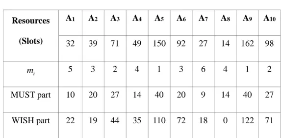
Before leaving this chapter, we use a simple example to describe the operation of our proposed algorithm. Assume that there are 12 time slots and 30 sub-channels in the DL sub-frame. The Mobile WiMAX system uses 6 MCSs: QPSK 1/2; QPSK 3/4; 16QAM 1/2; 16QAM 3/4; 64QAM 2/3; 64QAM 3/4 which have number of bytes per slot are 6, 9, 12, 18, 24, 27 and are converted to 6 modulation levels from 1 to 6, respectively. There are 10 MS and in each data request, a MCS is assigned randomly, urgent data size equal to 240 Bytes, and non-urgent data size is assigned randomly from 0 to 1520 Bytes. The set of all data request calculated in number of slots are shown in

Table 3.1.

Table 3.1 An example of proposed algorithm Resources (Slots) A1 A2 A3 A4 A5 A6 A7 A8 A9 A10 32 39 71 49 150 92 27 14 162 98 i m 5 3 2 4 1 3 6 4 1 2 MUST part 10 20 27 14 40 20 9 14 40 27 WISH part 22 19 44 35 110 72 18 0 122 71

In the first phase, after sorting the set of requests we have sorted_A =

7 1 4 8 6 2 10 3 9 5

{A A A A A A A, , , , , , ,A A A . The first iteration begins with selecting the first , , } strip K_1,12 that have the largest available space R1,12 





highest-priority request A₇ 27 (m₇ 6) . According to Step 3, we calculate

27 / 30 1

w_ _ , h_27 / 1_27, then the rectangle R





7

A . K1,12 K1,12 will be split into K1,1 and K2,12. The set will be updated as = 1,1 2,12

{K ,K }. In the second iteration, the maximum rectangle R2,12 





K is selected to map A₁32. According to Step 3, the rectangle R





is allocated to A . ₁ K2,12 is split into K2,3 and K4,12, and the set  is updated as = 1,1 2,3 4,12

{K ,K ,K }. The first phase is executed for 4 more iterations to map requests

4, 8, 6

A A A , and A . After finishing the first phase, we have sorted_A =2 {A10,A A A 3, 9, 5}

and ={K ,K ,K .K ,K_{1,1 2,3 4,5 6,9 10,11},K_12,12}.

In the first iteration of the second phase, we try to map M into ₁₀ Ki j, , for all ,

i j

K According to Step 2i) and Step 3, the rectangle R_6,9 _(6, 24); 4, 7_ in K_6,9

is used to allocate M . Similarly, in the second iteration, the rectangle ₁₀ R12,12 in K12,12

is used to allocate M (and a part of ₃ W ). In the third and fourth iteration, we choose ₃

10.11

K and K_4,5 to map M and ₉ M by returning the over allocated slots and some ₅

Fig. 3.2 An Example of DL data mapping using E-TLRM algorithm.

For this example, the MUST part, WISH part and unused slots are shown in dark gray, gray and white, respectively. The total number of over allocated slots (shown in black) is 1. All of the MUST data are mapped. The efficiency (percentage of used space over total space) of the proposed algorithm is 95%, with over allocated slots and unused slots being counted as wasted space. The final results of this example are shown as

Table 3.2.

Table 3.2 E-TLRM example results

Over allocated Slots 1

Unused Slots 17

Unmapped MUST parts 0

Chapter 4 Performance Evaluation

In this chapter, we present the simulation results to show numerical results comparing our proposed algorithm E-TLRM with eOCSA and TLRM algorithms. In our simulations, we assume that the request for each MS is randomly generated; with the constraint that the urgent and non-urgent traffics (in Bytes) are generated uniformly in [0,240] and in [0,1520] with different distributions and are converted to MUST parts and WISH parts (in slots), respectively. We also assume that the MCS of each MS is assigned randomly and one burst in DL sub-frame is allocated for each MS.

The number of MSs is randomly chosen from 1 to 36. The over allocated slots, unused slots, efficiency, number of mapped request’s MUST part and urgent data throughput are averaged out over 10000 trials. For our simulation, the physical bandwidth is 10 MHz and the frame duration is 5 ms. The duplexing technique is TDD, and the permutation mode is PUSC, which is the most commonly used mode. The simulations use 6 MCSs: QPSK 1/2; QPSK 3/4; 16QAM 1/2; 16QAM 3/4; 64QAM 2/3; 64QAM 3/4 which have number of bytes per slot are 6, 9, 12, 18, 24, 27 and are converted to 6 modulation levels from 1 to 6, respectively. A summarized description of the system simulation parameters are shown in Table 4.1.

Table 4.1 System simulation parameters

Parameter Value

Frame length 5 ms

Channel BW 10 MHz

Permutation scheme PUSC Number of sub-channels 30

DL sub-frame 12 slot columns Total number of slots per DL

sub-frame

30 x 12 slots

Modulation and Coding scheme (bytes/slot) QPSK 1/2( μ1=6 ) QPSK 3/4( μ2=9 ) 16QAM 1/2( μ3=12 ) 16QAM 3/4( μ4=18 ) 64QAM 2/3( μ5= 24) 64QAM 3/4( μ6=27 ) Urgent data 0 ~240 Bytes

Non-urgent data 0 ~1520 Bytes Simulation time 10000 frames

As mention before, the selected algorithms to compare our E-TLRM algorithm with is that of eOCSA and TLRM. We start by evaluating the impact of unused slots, which is defined as the fraction of the DL sub-frame taken by the slots that are left unused in certain frame.

Fig. 4.1 Average unused slots vs. number of MSs.

Fig. 4.1 shows that under the low traffic load (10 MSs), the E-TLRM algorithm generates more unused slots than TLRM algorithm. In the proposed algorithm, the requests with higher MCS levels that could be require smaller number of slots are mapped earlier. Consequently, unmapped requests in the second phase usually are of larger sizes and require some allocated WISH parts to be returned in order to map them into DL sub-frame. On average, the unused slots of E-TLRM are 11.385 and 0.392 with TLRM algorithm. When the number of MSs is high, the average of unused slots for both proposed algorithm and TLRM algorithm approach 0. In both cases, the average number of unused slots for the eOCSA algorithm is always higher than that of E-TLRM and TLRM.

In Fig. 4.2, we compare the over allocated slots of proposed algorithm with eOCSA and TLRM algorithms. As mentioned before, the over allocated slots is defined as the fraction of the DL sub-frame taken by the portions of the burst that are not actually

being utilized for data request.

Fig. 4.2 Average over allocated slots vs. number of MSs.

Since the proposed algorithm maps the requests with higher MCS level in the first phase, the number of strips is more than that of TLRM algorithm. As a result, our proposed E-TLRM algorithm generates more over allocated slots than TLRM algorithm as shown in Fig. 4.2.

From the analyses with average of unused slots and over allocated slots, it is easy to understand why the efficiency of the proposed algorithm is slightly worse than TLRM algorithm but is still better than eOCSA as can be seen in Fig. 4.3. The average efficiency is defined as allocated slots divided by total slots per frame.

Fig. 4.3 Average efficiency vs. number of MSs.

Furthermore, we compare the throughput and average amount of mapped MUST parts of proposed algorithm with eOCSA and TLRM algorithms.

Since eOCSA only considers the numbers of slots, it is possible that a MS with a worst MCS gets a highest priority and consumes a lot of slots. Without considering the traffic differentiation, the MUST part throughput of eOCSA saturates when the number of MSs is about 5, resulting in a flat curve in. TLRM can return some slots of WISH parts to allocate more MUST parts. We can see that the MUST part and throughput increases dramatically. Because E-TLRM determines the mapping order according to the MUST part’s size and MCS of each MS, it outperforms both eOCSA and TLRM algorithms in terms of the throughput and the average amount of mapped MUST parts.

Chapter 5 Conclusions

The main contribution of this thesis is to implement an enhanced version of the data mapping algorithm for two-level requests in IEEE 802.16e mobile WiMAX systems. We first introduce the data mapping problem in WiMAX system in Chapter 1. Then we briefly introduce the eOCSA and TLRM algorithms which proposed in literature to solve the data mapping problem in Chapter 2.

In Chapter 3, our proposed E-TLRM algorithm is described. E-TLTM, similar to previous algorithm TLRM, consists of two phases and can effectively prioritize the urgent traffic. The basic change of our proposed algorithm is that the mapping order is determined based on both the MCS and MUST part’s sizes. Simulation results in Chapter 4 show that the proposed algorithm outperforms previous schemes. The proposed algorithm can serve a larger number of MUST data requests and in the meantime achieves higher throughput than previous schemes.

Bibliography

[1] IEEE 802.16e-2005, “IEEE Standard for Local and metropolitan area networks - Part 16: Air Interface for Fixed and Mobile Broadband Wireless Access Systems - Amendment 2: Physical and Medium Access Control Layers for Combined Fixed and Mobile Operation in Licensed Bands and Corrigendum 1”, February 2006. [2] Cristina Ciochina and Hikmet Sari, “A Review of OFDMA and Single-Carrier

FDMA and Some Recent Results”, in Advances in Electronic and Telecommunications, vol. 1, no. 1, April 2010.

[3] Krishna Balachandran, Doru Calin, Fang-Chen Cheng, Niranjan Joshi, Joseph H. Kang, Achilles Kogiantis, Kurt Rausch, Ashok Rudrapatna, James P. Seymour, and Jonqyin Sun, “Design and Analysis of an IEEE 802.16e-Based OFDMA Communication System”, in Bell Labs Technical Journal, vol. 11, no. 4, pp. 53-73, 2007.

[4] WiMAX Forum, “WiMAX System Evaluation Methodology V2.1,” Jul. 2008, 230 pp. URL=http://www.wimaxforum.org/technology/documents.

[5] Yanqun Le, Yi Wu, and Dongmei Zhang, “An Improved Scheduling Algorithm for rtPS Services in IEEE 802.16”, IEEE VTC Sping 2009.

[6] C. So-In, R. Jain, and A. Al Tamimi, “Scheduling in IEEE 802.16e Mobile WiMAX Networks: Key Issues and a Servey”, in IEEE Journal on Selected Areas in Comm., vol. 27, no. 2, pp. 156-171, Feb. 2009.

[7] M-R Garey, and D-S Johnson, “Computers and Intractability: A Guide to the Theory of NP-Completeness”, W.H. Freeman, 340 pp., Jan. 1979.

Resource Allocation and Scheduling for Wireless OFDMA System with QoS Support”, EURASIP Journal on Wireless Communications and Networking Volume 2009, Article ID 134579, pages 12.

[9] T. Ali-Yahiya, A. Beylot, and G. Pujole, “Downlink Resource Allocation Strategies for OFDMA based Mobile WiMAX”, Telecommunication System, vol 44, no. 1-2, pp. 29-37, June 2010.

[10] A. Bacioccola, C. Cicconetti, L. Lenzini, E. Mingozzi, and A. Erta, “A Downlink Data Region Allocation Algorithm for IEEE 802.16e OFDMA”, 6th Interantion Conference on Information, Communication and Signal Processing, pp. 1-5, December 2007.

[11] T. Ohseki, M. Morita, and T. Inoue, “Burst Construction and Packet Mapping Scheme for OFDMA Downlinks in IEEE 806.16 System”, Proceeding of IEEE Global Communications Conference (IEEE GLOBECOM), 2009.

[12] Tsern-Huei Lee, Chi-Hsien Liu, Arleth Soleiy Garth Campbell, and Yaw-Wen Kuo, “A Data Mapping Algorithm for Two-Level Requests in WiMAX Systems”, IEEE VTC Sping 2012.

[13] C. So-In, R. Jain, and A. Al Tamimi, “OCSA: An Algorithm for Burst Mapping in IEEE 802.16e Mobile WiMAX Networks”, Proceedings of the 15th Asia-Pacific Conference on Communications (APCC 2009), Otc. 2009.

[14] C. So-In, R. Jain, and A. Al Tamimi, “eOCSA: An Algorithm for Burst Mapping with Strict QoS Requirements in IEEE 802.16e Mobile WiMAX Networks”, Proceedings of the 2nd IFIP Conference on Wireless Days, pp. 204-208, 2009.