急性中風病患就醫資料分析

(1)

國

立

交

通

大

學

統計學研究所

碩

士

論

文

急性中風病患就醫資料分析

Correlation of Arrival Time, Risk Factor and Prognosis in Acute

Stroke

研究生：黃崇豪

指導教授：王秀瑛博士

葉伯壽博士

(2)

急性中風病患就醫資料分析

Correlation of Arrival Time, Risk Factor and Prognosis in

Acute Stroke

研究生：黃崇豪 Student：Chong-Hao Huang

指導教授：王秀瑛博士 Advisor：Dr. Hsiuying Wang

葉伯壽博士 Advisor：Dr. Bak-Sau Yip

國立交通大學理學院

統計學研究所

碩士論文

A Thesis

Submitted to Institute of Statistics

College of Science National Chiao Tung University in partial Fulfillment of the Requirements

for the Degree of Master

in Statistics June 2012

Hsinchu, Taiwan, Republic of China

(3)

i

急性中風病患就醫資料分析

研究生：黃崇豪指導教授：王秀瑛博士

葉伯壽博士

國立交通大學統計學研究所碩士班

摘要

腦中風，又稱做腦血管疾病，一直是國人近年來死亡原因的前三名。患者在發現中風後三小時內靜脈注射血栓溶解劑可以有效治療缺血性腦中風，因此送醫時間一直是關注的重點。本文利用了台大醫院新竹分院的中風登錄表中於 2006 年至 2008 年所登錄的缺血中風患者的資料。我們研究了送醫方式與 NIHSS 之間的關係，以及送醫方式與送醫時間之間的關係。另外，我們也探討了送醫時間與診斷症狀、危險因子、病情變化、巴氏量表分數等之間的關係。關鍵字：腦中風、送醫時間、NIHSS 分數、危險因子、卡方檢定、t 檢定

(4)

ii

Correlation of Arrival Time, Risk Factor and Prognosis in

Acute Stroke

Student: Chong-Hao Huang Advisor: Dr. Hsiuying Wang

Dr. Bak-Sau Yip

Institute of Statistics National Chiao Tung University

Abstract

Stroke, also called cerebrovascular disease, is always the third most common cause of death in the recent year in Taiwan. Giving thrombolytic therapy within three hours of the first sign of stroke is efficient to help stroke patient limit stroke damage and disability. Therefore, the studies for the correlation of the arrival time and acute stroke and the correlation of the arrival way and acute stroke are important for thrombolytic therapy. In this thesis, we use the data from the stroke registry provided by the HsinChu General Hospital from 2006 to 2008. The relationship between NIHSS score and arrival ways, and the relationship between arrival time and arrival ways are investigated. In addition, we also explore the relationship between risk factors, Barthel index etc and the arrival time.

(5)

iii

誌謝

兩年前，帶著懵懂與不安的心情來到交大統研所；兩年後這樣的心情被不捨所取代。兩年說長不長說短也不短，但是卻也著實讓我學習到不少。首先，這篇論文的完成要感謝指導老師王秀瑛老師以及葉伯壽醫師。在論文的準備階段時王秀瑛老師總是不停的鼓勵我，在迷惑的時候也能夠適時的引導我前進一個方向，而葉伯壽醫師也在我不甚了解醫學方面的情況時可以幫助我了解情況，也確定我論文的方向。當然也要感謝新竹醫院神經科的李怡臻醫師再提供意見方面也有很大的幫助。感謝口試委員盧鴻興教授以及黃信誠教授的意見也使這篇論文更臻完善。再來感謝陪伴我度過這兩年的同學們，不管是在課業上的學習、還是私底下的玩鬧，我都覺得我獲得了許多以往沒有過的。宜靜、貓貓、小蜜蜂、阿鴻，你們的認真總是讓我覺得自己要認真；老大、亭育、偉振，你們的歡笑聲讓我不致於不安；終結、大鳥、魯夫、沒空，跟你們的聊天嘴砲真的是我在這兩年最快樂的時光。雖然要畢業了，但有你們我覺得來交大統計所的兩年是值得的。然後要感謝交大統計所上的老師們，有老師們的教導讓我在兩年學習到不少。也感謝所辦的郭姐及怡君姐也一直幫助我們處理一些瑣事，更要感謝家人在生活 上的支持以及鼓勵。最後真的很高興也很感謝交大統研對我們所提供的一切。 黃崇豪謹誌于國立交通大學統計學研究所中華民國一 O 一年六月

(6)

iv

List of Tables

Table 1. Analyses of the means of NIHSS score for the six pairs of the arrival ways. 25 Table 2. Analyses of the means of arrival time for the six pairs of the arrival ways. .. 26 Table 3. The comparison for the association of the arrival time within two hours and patients with symptom or sign during onset. ... 27 Table 4. The comparison for the association of the arrival time within two hours and patients with different symptoms or signs during onset. ... 28 Table 5. The comparison for the association of the arrival time within three hours and patients with symptoms or signs during onset. ... 29 Table 6. The comparison for the association of the arrival time within three hours and patients with different symptoms or signs during onset. ... 30 Table 7. The comparison for the proportions of two arrival time groups which one is less than two hours and another one is over two hours for patients with symptom or sign during onset... 31 Table 8. The comparison for the proportions of two arrival time groups which one is less than two hours and another one is over two hours for patients with different symptoms or signs during onset. ... 31 Table 9. The comparison for the proportions of two arrival time groups which one is less than three hours and another one is over three hours for patients with symptom or sign during onset... 32 Table 10. The comparison for the proportions of two arrival time groups which one is less than three hours and another one is over three hours for patients with different symptoms or signs during onset. ... 32 Table 11. The comparison for the association of the arrival time within two hours and patients with different risk factors. ... 33 Table 12. The comparison for the association of the arrival time within three hours and patients with different risk factors. ... 34 Table 13. The comparison for the proportions of two arrival time groups which one is less than two hours and another one is over two hours for patients with different risk factors. ... 35 Table 14. The comparison for the proportions of two arrival time groups which one is

(9)

vii

less than three hours and another one is over three hours for patients with different risk factors. ... 36 Table 15. The comparison for the association of the arrival time within two hours and patients with deterioration. ... 37 Table 16. The comparison for the association of the arrival time within two hours and patients with different deteriorations. ... 37 Table 17. The comparison for the association of the arrival time within three hours and patients with deterioration. ... 38 Table 18. The comparison for the association of the arrival time with three hours and patients with different deteriorations. ... 38 Table 19. The comparison for the proportions of two arrival time groups which one is less than two hours and another one is over two hours for patients with deteriorations. ... 39 Table 20. The comparison for the proportions of two arrival time groups which one is less than two hours and another one is over two hours for patients with different deteriorations. ... 39 Table 21. The comparison for the proportions of two arrival time groups which one is less than three hours and another one is over three hours for patients with deterioration. ... 40 Table 22. The comparison for the proportions of two arrival time groups which one is less than three hours and another one is over three hours for patients with different deteriorations. ... 40 Table 23. The comparison for the means of Barthel index of two arrival time groups which one is less than two hours and another one is over two hours for the difference of two stages. ... 41 Table 24. The comparison for the means of Barthel index of two arrival time groups which one is less than three hours and another one is over three hours for the difference of two stages. ... 42 Table 25. The comparison for the means of mRS of two arrival time groups which one is less than two hours and another one is over two hours for the difference of two stages. ... 43 Table 26. The comparison for the means of mRS of two arrival time groups which one is less than three hours and another one is over three hours for the difference of two stages. ... 44

(10)

viii

Figure

Figure 1. The means of Barthel index of two arrival time groups which one is less than two hours and another one is over two hours for the difference of two stages. ... 45 Figure 2. The means of Barthel index of two arrival time groups which one is less than three hours and another one is over three hours for the difference of two stages. ... 45 Figure 3. The means of mRS of two arrival time groups which one is less than two hours and another one is over two hours for the difference of two stages... 46 Figure 4. The means of mRS of two arrival time groups which one is less than three hours and another one is over three hours for the difference of two stages. ... 46

(11)

1

1. Introduction

1.1 Motivation

Stroke, also named cerebrovascular disease, is a major cause of long-term physical, cognitive, emotional, and social disability. It is also the third most common cause of death, after cancer and heart disease in Taiwan. The prevalence of stroke in Taiwan is about 16.42 per population [1]. According to the statistic data from the Department of Health, Executive Yuan, there were 10,134 people died of cerebrovascular disease and accounts for 7% of deaths in 2010 [2].

There are two types of stroke: ischemic stroke and hemorrhagic stroke. The incidences of different stroke in Taiwan are ischemic-67%, hemorrhagic-14%, subarachnoid hemorrhage-4% and unclassified-15% [3]. Most of the stroke patients are belong to ischemic stroke, which results from blood supply blockage to the brain by blood clots or fatty deposits called plaque in linings of blood vessel. For ischemic stroke, tissue plasminogen activator (TPA) is one of thrombolytic drugs that can be injected intravenous or intra-arterial within certain time window to restore blood flow to brain. The best time window for thrombolytic drugs is within three hours from the first signs of stroke, which reduced in death or dependency. The time interval between the first sign of stroke and the hospital arrival called the arrival time is most important. The shorter the arrival time will cause the more efficient of the thrombolytic therapy [4-5].

Though the arrival time is important for thrombolytic therapy, it is hardly to be discussed for data scarcity in Taiwan [6-7]. From 2006 to 2008, the stroke patients in

(12)

2

HsinChu General Hospital are registered in detail from their arrival to discharge under the stroke registry porgramme. We analyzed and evaluated the informations to discuss factors on arrival time and stroke patient dependency as they discharged.

1.2 Outline

The purpose of the thesis is to discuss the association between the arrival time and the National Institutes of Health Stroke Scale (NIHSS) score and risk factors in patients with cerebrovascular disease patients. In Chapter 2, we introduce the type of stroke and the factors, including NIHSS score and arrival way, symptom or sign during onset and risk factor, deterioration, Barthel index and mRS score. Furthermore, we review some literatures for discussing the related subject. In Chapter 3, we introduce all the methods we used for the analysis of the different data type. Chapter 4 presents the result of our analysis. And in Chapter 5, we have some conclusions for our study.

(13)

3

2. Literature Review

2.1 Introduction of Stroke

Stroke is the rapid loss of brain functions due to blood supply blockage to the brain tissue. The affected area of the different part of the brain results in limbs paralysis, visual loss, aphasia or apraxia.

There are two types of strokes: ischemic strokes and hemorrhagic strokes. The incidences of different stroke in Taiwan are ischemic-67%, hemorrhagic-14%, subarachnoid hemorrhage-4% and unclassified-15%. Most of the stroke patients are belong to ischemic stroke, which results from blood supply blockage to the brain by blood clots or fatty deposits called plaque in linings of blood vessel.

Hemorrhagic stroke includes intra-cerebral hemorrhage and subarachnoid hemorrhage. In intra-cerebral hemorrhage, bleeding occurs from vessels within the brain itself, and hypertension is the most common cause. Subarachnoid hemorrhage is bleeding in the area between the brain and the thin tissues that cover it, which usually results from rupture of an aneurysm.

Either a blood clot that blocks an artery in ischemic strokes or an artery rupture, interrupting blood flow to an area of the brain in hemorrhagic strokes, brain cells begin to die and brain damage occurs. The brain is a complex organ and controls various body functions. When stroke leads to brain cells damage, the body function controlled by that part of the brain lost. The effects of a stroke depend on several factors, including the location of the brain damage area and how much brain tissue is affected. For example, strokes over left side of brain may cause paresis of right side

(14)

4 limbs, trouble speaking or understanding others.

To identify different kinds of strokes is essential because the treatment depends on the strokes type. After obtaining medical history, blood tests, and physical examination, Computed Tomography Scan is a good test for patients who were suspected having a stroke. Not only because it can easily detect bleeding inside the brain, but also because it can be performed quickly. Magnetic resonance imaging (MRI) can detect ischemic strokes, and Magnetic resonance angiography (MRA) can evaluate arteries in the neck and brain. Arteriography can be used to detect the site of vessel blockage or vessel abnormality. Furthermore, carotid ultrasound would also be arranged in ischemic strokes to evaluate narrowing in carotid arteries.

For ischemic strokes, the aim is to restore blood flow to brain. Tissue plasminogen activator (also called TPA) is a protein involved in the breakdown of blood clots, and is the only clot-busting drug. It can be injected intravenous or intra-arterial within certain time window [8]. Strict criteria apply and not all strokes patients are eligible. Other medication for ischemic strokes included antiplatelet agents such as aspirin, clopidogrel, and anticoagulant agents like heparin or warfarin. Treatment of hemorrhagic strokes focuses on controlling bleeding and reducing pressure in the brain. Patients may need surgery to evacuate hematoma, clipping or embolization of the aneurysm.

The fatality rates after a first stroke are about 12% 1 week, 19% at 1month, 31% at 1 year and 60% at 5 years. The relative risk of death in stroke survivors is about twice the risk of general population [9].

(15)

5

2.2 The Behavior and Characteristic of Strokes Patients Before hospitalization

2.2.1 NIHSS and Arrival Way

NIH strokes scale is a standardized method used to measure the level of impairment caused by a stroke [10]. It usually used in clinical medicine and in research. In clinical medicine, it is during the assessment of whether or not the degree of disability caused by a given stroke merits treatment with tPA. In research, it allows for the objective comparison for efficacy across different strokes treatments and rehabilitation. The NIH strokes scale score measures six aspects of brain function, including consciousness, vision, sensation, movement, speech and language. A certain number of points are given for impairment uncovered during a focused neurological examination. A maximal score of 42 represents the most severe and devastating strokes. The patients who have the amputation and joint fusion unable are excluded in this study. The details of each item of NIHSS are as the following:

 1a. Level of Consciousness (LOC): tests stimulation. Graded from 0-3.

 1b. LOC Questions: tests the patient's ability to answer questions correctly. Graded from 0-2.

 1c. LOC Commands: tests the patient's ability to perform tasks correctly. Graded from 0-2.

 2. Best Gaze: tests horizontal eye movements. Graded from 0-2.

 3. Visual Field: tests visual fields. Graded from 0-3.

 4. Facial Palsy: tests the patient's ability to move facial muscles. Graded from 0-3.

(16)

6

 5a. Motor Arm Left: tests motor abilities of the left arms. Graded from 0-4.

 5b. Motor Arm Right: tests motor abilities of the right arms. Graded from 0-4.

 6a. Motor Leg Left: tests motor abilities of the left legs. Graded from 0-4.

 6b. Motor Leg Right: tests motor abilities of the right legs. Graded from 0-4.

 7. Limb Ataxia: tests coordination of muscle movements. Graded from 0-2.

 8. Sensory: tests sensation of the face, arms, and legs. Graded from 0-2.

 9. Best Language: tests the patient's comprehension and communication. Graded from 0-3.

 10. Dysarthria: tests the patient's speech. Graded from 0-2.

 11. Extinction and Inattention: tests patient's recognition of self. Graded from 0-2.

Arrival way is the way for patients, their families or friends to choose how to go to the hospital when the signs of the stroke happened. It includes that drove the car themselves or by other people, called an ambulance by EMS or hospital, visited out-patient department or strokes happened in hospital. A certain number is given for patient to choose one of the modes.

2.2.2 Symptoms and Signs During Onset and Risk Factor

The symptoms and signs during onset defined as the patient’s description and the doctor’s diagnosis while the patient arrived at the hospital. Symptoms and signs include headache, consciousness disturbance, vomiting, dizziness, vertigo, delirium and seizure.

Risk factors for stroke are characteristics of an individual. The effect of those risk factors on subsequent stroke incidence is usually additive or multiplicative. They are

(17)

7

including with healthy lifestyle and diet along with preventive medical care where appropriate can significantly reduce the risk of suffering a strokes. By modifying certain behaviors and getting treatment for risky medical conditions, many of the conditions that commonly lead to stoke can be prevent or control [11-12].

The risk factors registered in the stroke registry that provided by Taiwan Stroke Society are:  HT (Hypertension)  DM (Diabetes Mellitus)  Previous CVA  Previous TIA  Heart Disease  Uremia  Smoking habit  Alcohol habit  Vegetarian  Dyslipidemia  Polycythemia  Physical Inactivity

 Family History of stroke

 Birth Pill

(18)

8

 Snoring

 Depression

 Other

2.3 The Prognosis of Strokes Patients after Hospitalization

2.3.1 Deterioration

Many patients with stroke will get worse over the next few days. Stroke patients

with deterioration stay longer in hospital, become more disabled and need more institutional care than patients without progression [13].

2.3.2 Barthel Index and mRS

The Barthel scale is an ordinal scale used to measure performance in activities of daily living. It consists of 10 items that measure person's daily function specifically the activities of daily living and mobility. Each performance item is rated on this scale with a given number of points assigned to each level or ranking. The ten variables registered in the Barthel scale are:

 Feeding

 Transfers (moving from wheelchair to bed and return)

 Grooming

 Personal toilet use

(19)

9

 Walking on level surface

 Climbing stairs

 Dressing

 Bowels

 Bladder

The Barthel scale can be used to determine a baseline level of functioning and can be used to monitor improvement in activities of daily living over time. The scores for each of the items are summed to create a total score. A higher number is associated with a greater likelihood of being able to live at home with a degree of independence following discharge from hospital [14].

The modified Rankin Scale (also called mRS) is a scale used to measuring the degree of disability or dependence in the daily activities of people who have suffered a stroke. The original Rankin Scale was developed in Scotland in 1957 by Rankin. The Rankin Scale was modified by Prof. C. Warlow's group at Western General Hospital in Edinburgh in 1988 as part of a study of aspirin in stroke prevention (UK-TIA Study Group, 1988) and renamed the mRS. The assessment is carried out by asking the patient about their activities of daily living, including outdoor activities. The information about the patient's neurological deficits on examination, physical, mental performance, and speech should be combined to choose an applicable mRS scale. The scale runs from 0-6, running from perfect health without symptoms to death.

(20)

10

 0 - No symptoms.

 1 - No significant disability. Able to carry out all usual activities, despite some symptoms.

 2 - Slight disability. Able to look after own affairs without assistance, but unable to carry out all previous activities.

 3 - Moderate disability. Requires some help, but able to walk unassisted.

 4 - Moderately severe disability. Unable to attend to own bodily needs without assistance, and unable to walk unassisted.

 5 - Severe disability. Requires constant nursing care and attention, bedridden, incontinent.

(21)

11

3. Data and Method

3.1 Database

In this study, the stroke registry is derived from the National Taiwan University Hospital Hsinchu Branch in August 2006 to October 2009. In order to control and realize more the situation of the stroke patients, the stroke registry is provided from Taiwan Stroke Society in 2006. The enrolled standards of the case study are (1) stroke onset within 10 days after hospitalization, (2) the patients who take the CT or MRI examination. As the patient is enrolled, the characteristics, medical treatment, clinical characterization and other information of the stroke patients are registered by the attending physician and clinical nursing staff from the hospital inpatient registry.

There are 1296 patients hospitalized in the neurology ward or entered the emergency ward due to ischemic stroke or hemorrhagic stroke and they satisfied the enrolled standard of the registry at the National Taiwan University Hospital Hsinchu Branch. In order to realize the characteristic of the patients with injections of thrombolytic agents, the stroke patients without the final diagnosis of infarct and TIA are excluded. Therefore, there are 1049 actually patients used for analysis. On these patients, several data are not available for some characteristics or other information. The stroke patients are not counted in the analysis when the data of some interested characteristic or other information is missing in the registry.

The cost of hospitalization, the address of the patients and other information are the detail file provided by the Bureau of National Health Insurance from the hospital database. There is seen as different hospitalizations if it has the same patients

(22)

12

repeatedly stroke into discharged from hospital records.

3.2 Method

For the purpose of analysis of data, chi-square test, Fisher exact test and binomial test, two sample t-test and two sample paired t-test are used. These methods in this study are introduced in detail in the next several sections, which are referred to [15-16].

3.2.1 Chi-square Test, Fisher Exact Test and Comparing Two Proportions

In order to analyze the association between the arrival time groups and symptom or sign during onset, risk factor and deterioration, we adopt the chi-square test to analyses the data. First, the stroke patients are divided into two groups with the arrival time. One group is that the arrival time is less than three hours and another one is that the arrival time is over three hours. The stroke patients are not admitted in the groups when their arrival time is a missing data. Second, we construct a 2 x 2 contingency table to the data. Let the variable be the patient with or without specific symptoms corresponding to rows heading 2 state which we index by i (i = 1, 2). Let the variable be the group of the arrival time corresponding to the column with 2 groups which we index by j (j = 1, 2). Let Oij be the calculated number of each j group of patients and i

state of the patients with or without specific symptoms. Finally we apply the chi-square test in the contingency table to test the independence of the arrival time groups and the patients with or without the different specific symptoms. The hypothesis of the test at the level significance α = 0.05 is:

(23)

13

Ho: The arrival time is independent of specific symptom of the patients.

Ha: The arrival time is dependent of specific symptom of the patients.

For a 2 x 2 contingency table, the Chi Square statistic is calculated by the formula:

Under the null hypothesis, the 2 statistic has approximately a 2 distribution with 1 degree of freedom and the p-value is obtained. Similar, we also adopt the method to analysis the relationship of the symptoms and arrival time which is under two hours or over two hours.

If one of sample size in our contingency table is less than five, we adopt the Fisher exact test instead of the chi-square test. For the contingency table, the probability of any particular possible array of cell frequencies and given fixed values for the marginal totals is calculated by given the hyper geometric rule:

Under the original hypothesis, the two-tailed probability would be that the sum of the separate probabilities for the arrays of equal or greater disproportion at the other extreme.

Another interesting issue is to investigate whether the proportions of two arrival time groups which one is less than two or three hours and another one is over two or three hours for patients with symptom. The large sample of test of the binomial variable is used to test. Suppose that the number of the patients with symptom which the arrival time is less two or three hours and the number of the patients with symptom which the arrival time is over two or three hours are the binomial variable.

(24)

14

We denote the first binomial variable is of size with the probability that estimated by the sample proportion and the other binomial variable proportion

estimates by from a sample of size , where

,

, and . By comparing the proportions, the mean and

variance are given by

The hypothesis of a two-sided test at the significance level α = 0.05 is:

Ho:

Ha:

The test statistic z is calculated by the formula:

Under the null hypothesis, the test statistic has approximately a standard normal distribution by the Central Limit Theorem for large and and the p-value is obtained.

3.2.2 Two Sample T-test

In order to analyze the difference of the NIHSS score and arrival time in different ways to hospital when the sign of the stroke has found, two-sample t-test is used. We also use two-sample t-test to test the means of Barthel index and the means of mRS score with the difference of two stages between the two arrival time groups. Before

(25)

15

testing for difference between two means, the variances of patients with NIHSS score and arrival time of two different arrived hospitals should be tested first. The stroke patients are not admitted when they has missing data in the factors we test. Denote the number of the admitted stroke patients of four ways to hospital n n n and n Denote y as the jth (j = , …, ni) patient of NIHSS score and arrival time

with the ith (i = 1, 2, 3, 4) way to hospital. Calculate the standard deviation

The hypothesis of each factor is:

0

_a

The test statistic t calculated by the formula is:

Under the null hypothesis, the test statistic F has approximately an F distribution with n n degree of freedom and the p-value is obtained. As the p-value is less than the significance level α = 0.05, we reject 0, resulting the inequality of the

two variances. On the contrary, we can assume that the two variances are equal when the p-value is larger than the significance level α = 0.05.

Second, we test the difference between two means of patients with NIHSS score and arrival time of each two different arrival way to hospitals. Calculate the means of y .

The hypotheses of testing the means of the NIHSS score for different factors are:

₀ 0 a

(26)

16

The hypotheses of testing the means of the arrival time for different factors are:

0 0

_a

According to the assumptions we made after testing the difference of the two variances, the statistic t calculated by the different formulas. As the variances are equal, the pooled variance is calculated to use as the best estimate of :

n n

n n And the test statistic is:

_n _n

Under the null hypothesis, the test statistic t has approximately a t distribution with degrees of freedom n n . As the variances are not equal, the estimated variance

is calculated with the two separate variances instead of with a pooled variance:

n n 0

And the test statistic is:

Under the null hypothesis, the test statistic t has approximately a t distribution with degrees of freedom . atterthwaite and cheffe’ appro imated the distribution of

(27)

17 n n _n n _n n

However, is usually not an integer, so the closet integer to is used as the degrees of freedom and the p-valued is obtained.

(28)

18

4. Result

4.1 NIHSS Score Associated with Prehospital Delay and Arrival Way

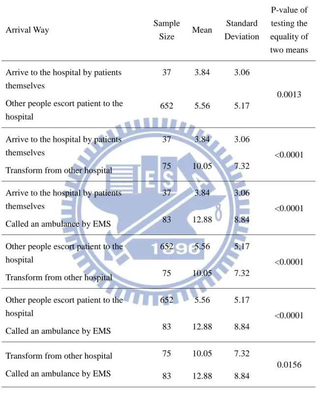
We use the t-test to test the difference of NIHSS score means associated with the arrival ways. Table 1 shows the result for the two sample t-test of NIHSS score for the six pairs of the arrival ways. According to Table 1, all the means are significant at level α=0.05. We conclude that the mean of NIHSS score of the arrival way is the largest in patient sent by 119, followed by transformed from other hospital, sent by their family and arrived to the hospital by themselves.

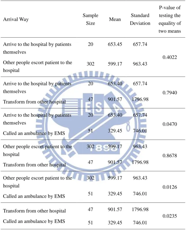
We use the t-test to test the difference of arrival time means associated with the arrival ways. Table 2 shows the result for the two sample t-test of arrival time for the six pairs of the arrival ways. According to Table 2, the mean of the arrival time between patient sent by 119 and other arrival ways are significant to the alternative hypotheses at level α=0.05. We conclude that the patient sent by 119 is the fast than other arrival ways.

4.2 Symptoms and Risk Factors Associated With the Arrival Time

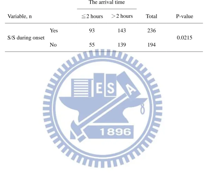
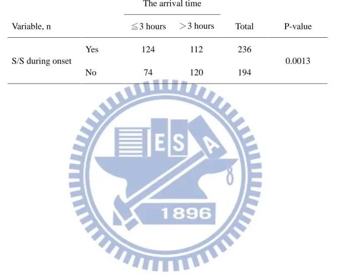
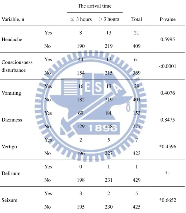
Tables 3 and 4 are the comparison for the association of the arrival time with two hours and patients with symptom or sign during onset. Tables 5 and 6 are the comparison for the association of the arrival time with three hours and patients with symptom or sign during onset. According to the Tables 3 and 5, the p-values are small enough to reject the null hypothesis at level α=0.05. We conclude that the patients with or without S/S during onset is associated with the arrival time groups. According

(29)

19

to the Tables 4 and 6, the p-values of are significant for the patient with cons disturbance at level α=0.05. We conclude that patient with cons disturbance is associated with the arrival groups.

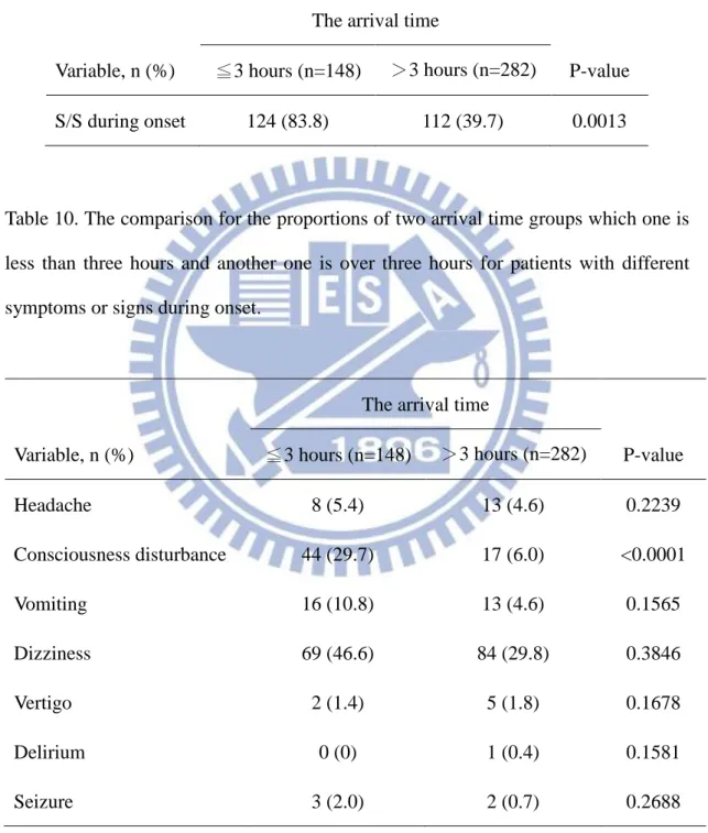
Tables 7 and 8 show the proportions of two arrival time groups which one is less than two hours and another one is over two hours for patients with symptom or sign during onset. Tables 9 and 10 show the proportions of two arrival time groups which one is less than three hours and another one is over three hours for patients with symptom or sign during onset. According to the Tables 7 and 9, the p-values are small enough to reject the null hypothesis at level α=0.05. We conclude that the proportion of arrival time less than two or three hours is difference from the proportion of arrival time over than two or three hours. According to the Tables 8 and 10, the two proportions of two arrival time groups are different only depend on patient with consciousness disturbance with p-values are all less than 0.0001.

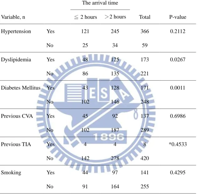
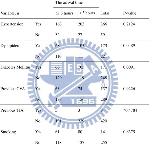
Tables 11 and 12 are the comparison for the association of the two different arrival time groups and patients with different risk factors. Tables 13 and 14 show the proportions of the two different arrival time groups for patients with different risk factors. According to Tables 11 and 12, the p-values of are significant for the patient with dyslipidemia or diabetes mellitus at level α=0.05. We conclude that patient with dyslipidemia or diabetes mellitus is associated with the arrival groups. According to the Table 13, the two proportions of two arrival time groups are different depend on patient with dyslipidemia or diabetes mellitus with p-values are 0.0089 and 0.0002. According to the Table 14, we also have the same conclusion with the p-value 0.0184 and 0.0031.

(30)

20

4.3 Deterioration, Barthel Index and mRS Associated with The Arrival Time

Tables 15 and 16 are the comparison for the association of the arrival time with two hours and patients with deterioration. Tables 17 and 18 are the comparison for the association of the arrival time with three hours and patients with deterioration. According to the Tables 15 and 17, the p-values are not rejected to the null hypothesis at level α=0.05. We conclude that the patients with or without deterioration is not associated with the arrival time groups. According to the Tables 16 and 18, the p-values of are all not significant for the patient with different deteriorations at level α=0.05. We conclude that patient with different deteriorations are not associated with the arrival groups.

Tables 19 and 20 show the proportions of two arrival time groups which one is less than two hours and another one is over two hours for patients with different deteriorations. Tables 21 and 22 show the proportions of two arrival time groups which one is less than three hours and another one is over three hours for patients with deterioration. According to the Tables 19 and 21, the p-values are all not small enough to reject the null hypothesis at level α=0.05. We conclude that the proportion of arrival time less than two or three hours is not difference from the proportion of arrival time over than two or three hours for patient with deterioration. According to the Tables 20 and 22, the p-values are all not small enough to reject the null hypothesis at level α=0.05. We conclude that the two proportions of two arrival time groups are all different for patient with different deterioration.

Table 23 and Figure 1 show the means of Barthel index of two arrival time groups which one is less than two hours and another one is over two hours for the difference

(31)

21

of two stages. Table 24 and Figure 2 show the means of Barthel index of two arrival time groups which one is less than three hours and another one is over three hours for the difference of two stages. According to the Tables 23 and 24, the p-values are all not small enough to reject the null hypothesis at level α=0.05. We conclude that the mean of arrival time less than two or three hours is not different to the mean of arrival time over than two or three hours for the difference of two stages.

Table 25 and Figure 3 show the means of mRS of two arrival time groups which one is less than two hours and another one is over two hours for the difference of two stages. Table 26 and Figure 4 show the means of mRS of two arrival time groups which one is less than three hours and another one is over three hours for the difference of two stages. But according to the Tables 25 and 26, only the p-value for patient from one month after stroke to three month after stroke is small enough to reject the null hypothesis at level α=0.05. We conclude that the means of arrival time groups are different only depend on the two stages for patient from one month after stroke to three months after stroke.

(32)

22

5. Conclusion

We find out the arrival way that patient call the ambulance by EMS (119) has the shortest arrival time. We also find out the arrival way that patient sent to the hospital by 119 has the largest NIHSS score (severity), followed by patient transformed from other hospital, sent by other people and arrived hospital by themselves.

The arrival time depends on the patient with or without consciousness disturbance. It also depends on the patient with or without dyslipidemia or diabetes mellitus. But it does not depend on the patient with or without different deteriorations. There is also a difference of the proportions between two arrival time groups. One is less than two or three hours and another one is over two or three hours for the patient with the dependent factors.

For the relationship of the arrival time and prognostic, the arrival time does not depend on the difference of prognostic for two stages with the Barthel index. But the arrival time depends on the difference of prognostic between the mRS of patient with stroke after one month and the mRS of patient with stoke after three months.

(33)

23

References

[1] Huang, Z.- S., Chiang, T.-L. and Lee, T.-K. ( ), “ troke Prevalence in Taiwan Findings from the National ealth Interview urvey”, Stroke, 28:1579-1584.

[2] 行政院衛生署網站 (2007)。http://www.doh.gov.tw/statistic/index.htm。

[3] Hu, H.-H., Sheng, W.-Y., Chu, F.-L., et al. (1992), “Incidence of stroke in Taiwan.”, Stroke, 23:1237-1241.

[4] Debra KM, Laura PK, Mark JA, et al. ( 006), “Reducing delay in seeking treatment by patients with acute coronary syndrome and stroke: A scientific statement from the American heart association council on cardiovascular Nursing and stroke coucil”, Circulation, 114:168-182.

[5] Fang, J., Yan, W., Jiang, G.- ., et al. ( 0 ), “Time interval between stroke onset and hospital arrival in acute ischemic stroke patients in hanghai, China”, Clinical

Neurology and Neurosurgery, 113:85-88.

[6] Tan, T.-Y., Chang, K.-C. and Liou, C.-W. (2002), “Factors delaying hospital arrival after acute stroke in southern Taiwan”, Chang Gung Medicine, 25:458-463.

[7] Chang, K.-C., Tseng, M.-C., Tan, T.-Y. (2004), “Prehospital Delay After Acute Stroke in Kaohsiung, Taiwan”, Stroke, 35:700-704.

[8] Inatomi, Y., Yonehara, T., Hashimoto, Y., et al. (2008), “Pre-hospital delay in the use of intravenous rt-PA for acute ischemic stroke in Japan”, The Journal of

Neurological Sciences, 270:127-132.

[9] Hankey GJ, Jamrozil, Broadhurst RJ et al. (2000), “Five-year survival after first-ever stroke and related prognostic”, Stroke, 31:2080-2086.

(34)

24

[10] Brott, TG, Adams HP, Olinger CP, et al. (1989), “Measurements of acute cerebral infarction: a clinical e amination scale.”, Stroke, 20:864-870.

[11] Hyung, J.-K., Jung, H.-A., Sun, H.-K., et al. (2011), “Factors associated with prehospital delay for acute stroke in Ulsan, Korea”, The Journal of Emergency

Medicine, 41:59-63.

[12] Yuko, T., Makoto, N., Teruyuki, H., et al. (2009), “Factors influencing pre-hospital delay after ischemic stroke and transient ischemic attack”, Internal

Medicine, 48:1739-1744.

[13] Lee, H.-C., Chang, K.-C., Lan, C.-F., et al. (2008), “Factors associated with prolonged hospital stay for acute stroke in Taiwan”, Acta Neurologica Taiwanica, 17:17-25.

[14] Kim, Y.-S., Park, S.-S. Bae, H.-J., et al. (2011), “ troke awareness decreases prehospital delay after acute ischemic stroke in korea”, BMC Neurology, 11:2.

[15] Jerrold, H. Zar. (2009). Biostatistical Analysis, Fifth Edition. Pearson International Edition.

[16] Llord D. Fisher, Gerald Van Belle (1996). Biostatistics: A Methodology For The

(35)

25

Table 1. Analyses of the means of NIHSS score for the six pairs of the arrival ways.

Arrival Way Sample

Size Mean Standard Deviation P-value of testing the equality of two means

Arrive to the hospital by patients themselves

Other people escort patient to the hospital

37 3.84 3.06

0.0013 652 5.56 5.17

Transform from other hospital

37 3.84 3.06

<0.0001 75 10.05 7.32

Called an ambulance by EMS

37 3.84 3.06

<0.0001 83 12.88 8.84

652 5.56 5.17

<0.0001 75 10.05 7.32

652 5.56 5.17

<0.0001 83 12.88 8.84

Transform from other hospital Called an ambulance by EMS

75 10.05 7.32

0.0156 83 12.88 8.84

(36)

26

Table 2. Analyses of the means of arrival time for the six pairs of the arrival ways.

Arrival Way Sample

Size Mean Standard Deviation P-value of testing the equality of two means

20 653.45 657.74

0.4022 302 599.17 963.43

20 653.40 657.74

0.7940 47 901.57 1796.98

20 653.40 657.74

0.0470 51 329.45 746.01

302 599.17 963.43

0.8678 47 901.57 1796.98

302 599.17 963.43

0.0126 51 329.45 746.01

Transform from other hospital Called an ambulance by EMS

47 901.57 1796.98

0.0235 51 329.45 746.01

(37)

27

Table 3. The comparison for the association of the arrival time within two hours and patients with symptom or sign during onset.

Variable, n

The arrival time

Total P-value ≦2 hours ＞2 hours S/S during onset Yes 93 143 236 0.0215 No 55 139 194

(38)

28

Table 4. The comparison for the association of the arrival time within two hours and patients with different symptoms or signs during onset.

Variable, n

The arrival time

Total P-value ≦ 2 hours ＞2 hours Headache Yes 6 15 21 0.7317 No 142 267 409 Consciousness disturbance Yes 38 23 61 <0.0001 No 110 259 369 Vomiting Yes 14 15 29 0.1544 No 134 267 401 Dizziness Yes 49 104 153 0.5028 No 99 178 277 Vertigo Yes 1 6 7 *0.4303 No 147 276 423 Delirium Yes 0 1 1 *1 No 148 281 429 Seizure Yes 2 3 5 *1 No 146 279 425

(39)

29

Table 5. The comparison for the association of the arrival time within three hours and patients with symptoms or signs during onset.

Variable, n

The arrival time

Total P-value ≦3 hours ＞3 hours S/S during onset Yes 124 112 236 0.0013 No 74 120 194

(40)

30

Table 6. The comparison for the association of the arrival time within three hours and patients with different symptoms or signs during onset.

Variable, n

The arrival time

Total P-value ≦ 3 hours ＞3 hours Headache Yes 8 13 21 0.5995 No 190 219 409 Consciousness disturbance Yes 44 17 61 <0.0001 No 154 215 369 Vomiting Yes 16 13 29 0.4076 No 182 219 401 Dizziness Yes 69 84 153 0.8475 No 129 148 277 Vertigo Yes 2 5 7 *0.4596 No 196 227 423 Delirium Yes 0 1 1 *1 No 198 231 429 Seizure Yes 3 2 5 *0.6652 No 195 230 425

(41)

31

Table 7. The comparison for the proportions of two arrival time groups which one is less than two hours and another one is over two hours for patients with symptom or sign during onset.

Variable, n (%)

The arrival time

P-value ≦2 hours (n=148) ＞2 hours (n=282)

S/S during onset 93 (62.8) 143 (50.7) 0.0073

Table 8. The comparison for the proportions of two arrival time groups which one is less than two hours and another one is over two hours for patients with different symptoms or signs during onset.

Variable, n (%)

The arrival time

P-value ≦2 hours (n=148) ＞2 hours (n=282) Headache 6 (4.1) 15 (5.3) 0.2735 Consciousness disturbance 38 (25.7) 23 (8.2) <0.0001 Vomiting 14 (9.5) 15 (5.3) 0.0662 Dizziness 49 (33.1) 104 (36.9) 0.2169 Vertigo 1 (0.7) 6 (2.1) 0.0918 Delirium 0 (0) 1 (0.4) 0.1582 Seizure 2 (1.4) 3 (1.1) 0.3995

(42)

32

Table 9. The comparison for the proportions of two arrival time groups which one is less than three hours and another one is over three hours for patients with symptom or sign during onset.

Variable, n (%)

The arrival time

S/S during onset 124 (83.8) 112 (39.7) 0.0013

Table 10. The comparison for the proportions of two arrival time groups which one is less than three hours and another one is over three hours for patients with different symptoms or signs during onset.

Variable, n (%)

The arrival time

P-value ≦3 hours (n=148) ＞3 hours (n=282) Headache 8 (5.4) 13 (4.6) 0.2239 Consciousness disturbance 44 (29.7) 17 (6.0) <0.0001 Vomiting 16 (10.8) 13 (4.6) 0.1565 Dizziness 69 (46.6) 84 (29.8) 0.3846 Vertigo 2 (1.4) 5 (1.8) 0.1678 Delirium 0 (0) 1 (0.4) 0.1581 Seizure 3 (2.0) 2 (0.7) 0.2688

(43)

33

Table 11. The comparison for the association of the arrival time within two hours and patients with different risk factors.

Variable, n

The arrival time

Total P-value ≦ 2 hours ＞2 hours Hypertension Yes 121 245 366 0.2112 No 25 34 59 Dyslipidemia Yes 48 125 173 0.0267 No 86 135 221

Diabetes Mellitus Yes 43 128 171 0.0011

No 102 146 248

Previous CVA Yes 45 92 137 0.6986

No 102 187 289

Previous TIA Yes 4 4 8 *0.4533

No 142 278 420

Smoking Yes 44 97 141 0.4295

No 91 164 255

(44)

34

Table 12. The comparison for the association of the arrival time within three hours and patients with different risk factors.

Variable, n

The arrival time

Total P-value ≦ 3 hours ＞3 hours Hypertension Yes 163 203 366 0.2124 No 32 27 59 Dyslipidemia Yes 68 105 173 0.0489 No 110 111 221

Diabetes Mellitus Yes 66 105 171 0.0091

No 129 119 248

Previous CVA Yes 63 74 137 0.9226

No 133 156 289

Previous TIA Yes 5 3 8 *0.4784

No 191 229 420

Smoking Yes 61 80 141 0.6375

No 118 137 255

(45)

35

Table 13. The comparison for the proportions of two arrival time groups which one is less than two hours and another one is over two hours for patients with different risk factors.

Variable, n (Total, %)

The arrival time

P-value ≦2 hours ＞2 hours Hypertension 121 (146, 82.9) 245 (279, 87.8) 0.0900 Dyslipidemia 48 (134, 35.8) 125 (260, 48.1) 0.0089 Diabetes Mellitus 43 (145, 29.7) 128 (274, 46.7) 0.0002 Previous CVA 45 (147, 30.6) 92 (279, 33.0) 0.3087 Previous TIA 4 (146, 2.7) 4 (282, 1.4) 0.1929 Smoking 44 (135, 32.6) 97 (261, 37.2) 0.1813

(46)

36

Table 14. The comparison for the proportions of two arrival time groups which one is less than three hours and another one is over three hours for patients with different risk factors.

Variable, n (Total, %)

The arrival time

P-value ≦3 hours ＞3 hours Hypertension 163 (195, 83.6) 203 (230, 88.3) 0.0846 Dyslipidemia 68 (178, 38.2) 105 (216, 48.6) 0.0184 Diabetes Mellitus 66 (195, 33.9) 105 (224, 46.9) 0.0031 Previous CVA 63 (196, 32.1) 74 (230, 32.2) 0.4973 Previous TIA 5 (196, 2.6) 3 (232, 1.3) 0.1755 Smoking 61 (179, 34.1) 80 (217, 36.9) 0.2817

(47)

37

Table 15. The comparison for the association of the arrival time within two hours and patients with deterioration.

Variable, n

The arrival time

Total P-value ≦2 hours ＞2 hours Deterioration Yes 24 46 70 0.9109 No 124 236 360

Table 16. The comparison for the association of the arrival time within two hours and patients with different deteriorations.

Variable, n

The arrival time

Total P-value ≦ 2 hours ＞2 hours Stroke-in-evolution Yes 18 41 59 0.5940 No 130 241 371 Herniation Yes 0 0 0 Na No 148 282 430 Hemorrhagic Infarct Yes 4 4 8 *0.4551 No 144 278 422 Medical Problem Yes 0 0 0 Na No 148 282 430 Other Yes 2 1 3 *0.2734 No 146 281 427

(48)

38

Table 17. The comparison for the association of the arrival time within three hours and patients with deterioration.

Variable, n

The arrival time

Total P-value ≦3 hours ＞3 hours Deterioration Yes 31 39 70 0.8478 No 167 193 360

Table 18. The comparison for the association of the arrival time with three hours and patients with different deteriorations.

Variable, n

The arrival time

Total P-value ≦ 3 hours ＞3 hours Stroke-in-evolution Yes 24 35 59 0.4532 No 174 197 371 Herniation Yes 0 0 0 Na No 198 232 430 Hemorrhagic Infarct Yes 5 3 8 *0.4792 No 193 229 422 Medical Problem Yes 0 0 0 Na No 198 232 430 Other Yes 2 1 3 *0.5968 No 196 231 427

(49)

39

Table 19. The comparison for the proportions of two arrival time groups which one is less than two hours and another one is over two hours for patients with deteriorations.

Variable, n (%)

The arrival time

Deterioration 24 (16.2) 46 (16.3) 0.4898

Table 20. The comparison for the proportions of two arrival time groups which one is less than two hours and another one is over two hours for patients with different deteriorations.

Variable, n (%)

The arrival time

P-value ≦2 hours (n=148) ＞2 hours (n=282) Stroke-in-evolution 18 (12.2) 41 (14.5) 0.2429 Herniation 1 (0.7) 0 (0.0) 0.1578 Hemorrhagic Infarct 5 (3.4) 4 (1.4) 0.1165 Other 2 (1.4) 1 (0.4) 0.1626

(50)

40

Table 21. The comparison for the proportions of two arrival time groups which one is less than three hours and another one is over three hours for patients with deterioration.

Variable, n (%)

The arrival time

Deterioration 31 (15.7) 39 (16.8) 0.3730

Table 22. The comparison for the proportions of two arrival time groups which one is less than three hours and another one is over three hours for patients with different deteriorations.

Variable, n (%)

The arrival time

P-value ≦3 hours (n=198) ＞3 hours (n=232) Stroke-in-evolution 24 (12.1) 35 (15.1) 0.1846 Herniation 1 (0.5) 0 (0.0) 0.1580 Hemorrhagic Infarct 5 (3.0) 3 (1.3) 0.1116 Other 2 (1.0) 1 (0.4) 0.2429

(51)

41

Table 23. The comparison for the means of Barthel index of two arrival time groups which one is less than two hours and another one is over two hours for the difference of two stages.

Stage, mean

The arrival time

P-value of testing the equality of two means ≦ 2 hours ＞2 hours Stage 1 to Stage 2 3.089 4.269 0.3412 Stage 1 to Stage 3 3.171 3.580 0.7603 Stage 1 to Stage 4 1.667 1.356 0.7217 Stage 1 to Stage 5 -4.000 -3.223 0.7408 Stage 2 to Stage 3 6.322 8.069 0.3476 Stage 3 to Stage 4 8.898 9.323 0.8234 Stage 4 to Stage 5 5.120 6.524 0.6751

*Stage 1: Patient discharged from the hospital. Stage 2: Patient with stroke after one month.

Stage 3: Patient with stroke after three months. Stage 4: Patient with stroke after six months. Stage 5: Patient with stroke after one year.

(52)

42

Table 24. The comparison for the means of Barthel index of two arrival time groups which one is less than three hours and another one is over three hours for the difference of two stages.

Stage, mean

The arrival time

P-value of testing the equality of two means ≦ 3 hours ＞3 hours Stage 1 to Stage 2 3.423 4.255 0.4722 Stage 1 to Stage 3 3.533 3.374 0.8959 Stage 1 to Stage 4 1.242 1.641 0.6334 Stage 1 to Stage 5 -4.646 -2.536 0.3028 Stage 2 to Stage 3 7.012 7.968 0.6128 Stage 3 to Stage 4 8.797 9.482 0.7043 Stage 4 to Stage 5 4.000 7.701 0.2213

(53)

43

Table 25. The comparison for the means of mRS of two arrival time groups which one is less than two hours and another one is over two hours for the difference of two stages.

Stage, mean

The arrival time

P-value of testing the equality of two means ≦ 2 hours ＞2 hours Stage 1 to Stage 2 -0.146 -0.261 0.0694 Stage 1 to Stage 3 -0.154 -0.244 0.1432 Stage 1 to Stage 4 -0.067 -0.085 0.7448 Stage 1 to Stage 5 0.047 0.078 0.7928 Stage 2 to Stage 3 -0.306 -0.500 0.0245 Stage 3 to Stage 4 -0.407 -0.575 0.0795 Stage 4 to Stage 5 -0.361 -0.524 0.3060

(54)

44

Table 26. The comparison for the means of mRS of two arrival time groups which one is less than three hours and another one is over three hours for the difference of two stages.

Stage, mean

The arrival time

P-value of testing the equality of two means ≦ 3 hours ＞3 hours Stage 1 to Stage 2 -0.179 -0.260 0.1591 Stage 1 to Stage 3 -0.168 -0.252 0.1500 Stage 1 to Stage 4 -0.075 -0.082 0.8867 Stage 1 to Stage 5 0.088 0.051 0.7203 Stage 2 to Stage 3 -0.348 -0.507 0.0471 Stage 3 to Stage 4 -0.449 -0.575 0.1823 Stage 4 to Stage 5 -0.373 -0.547 0.2426

(55)

45

Figure 1. The means of Barthel index of two arrival time groups which one is less than two hours and another one is over two hours for the difference of two stages.

Figure 2. The means of Barthel index of two arrival time groups which one is less than three hours and another one is over three hours for the difference of two stages.

(56)

46

Figure 3. The means of mRS of two arrival time groups which one is less than two hours and another one is over two hours for the difference of two stages.

Figure 4. The means of mRS of two arrival time groups which one is less than three hours and another one is over three hours for the difference of two stages.

急性中風病患就醫資料分析

國

立

交

通

大

學

統計學研究所

碩

士

論

文

急性中風病患就醫資料分析

Correlation of Arrival Time, Risk Factor and Prognosis in Acute

Stroke

研 究 生：黃崇豪

指導教授：王秀瑛 博士

葉伯壽 博士

急性中風病患就醫資料分析

Correlation of Arrival Time, Risk Factor and Prognosis in

Acute Stroke

研 究 生：黃崇豪 Student：Chong-Hao Huang

指導教授：王秀瑛 博士 Advisor：Dr. Hsiuying Wang

葉伯壽 博士 Advisor：Dr. Bak-Sau Yip

國 立 交 通 大 學 理 學 院

統 計 學 研 究 所

碩 士 論 文

急性中風病患就醫資料分析

研究生：黃崇豪 指導教授：王秀瑛 博士

葉伯壽 博士

國立交通大學統計學研究所碩士班

摘要

Correlation of Arrival Time, Risk Factor and Prognosis in

Acute Stroke

Student: Chong-Hao Huang Advisor: Dr. Hsiuying Wang

Dr. Bak-Sau Yip

Abstract

誌謝

Contents

List of Tables

Figure

1. Introduction

2. Literature Review

3. Data and Method

4. Result

5. Conclusion

References

研究生：黃崇豪

指導教授：王秀瑛博士

葉伯壽博士

研究生：黃崇豪 Student：Chong-Hao Huang

指導教授：王秀瑛博士 Advisor：Dr. Hsiuying Wang

葉伯壽博士 Advisor：Dr. Bak-Sau Yip

國立交通大學理學院

統計學研究所

碩士論文

研究生：黃崇豪指導教授：王秀瑛博士

葉伯壽博士