Fuzzy neural network approach for 2-D direction finding in multipath environments

(1)

Fuzzy neural netw

finding in multipath environments

approach for 2-D direction

C.W.Ma and C.C.Teng

Abstract: A fuzzy neural network (FNN) approach for estimating the two-dimensional (2-D) direction of a radiating source in coherent multipath environments via a 2-D passive sensor array is presented. Outputs of the array are preprocessed by a judiciously constructed reference-point preprocessing scheme to produce proper inputs for an FNN. The FNN then uses these preprocessed outputs to produce the estimate of the source direction. Since the preprocessed outputs preserve enough information about the source direction and the FNN maps the preprocessed outputs into the source direction with high accuracy, the FNN approach exhibits good estimation performance. By computer simulations, it is found that the FNN approach drastically outperforms the spatial smoothing 2-D MUSIC algorithm.

1 Introduction

Finding the direction of a radiating source is an important task in sensor array signal processing. Applications of such a technique are versatile, including radar, sonar, multiuser mobile communication systems, etc. Researchers have published some remarkable works in the past twenty years. Among these works, the MUSIC algorithm [I], ESPRIT algorithm [2], weighted subspace fitting [3], MODE algorithm [4], etc., have received a lot of attention. These algorithms are generally based on an eigen-decom- position of the array’s output covariance matrix. As a result, the computational cost is expensive when the array size is large. The high computational cost makes these algorithms difficult to implement for a real-time environment. Recently, some researchers have become interested in using a fuzzy system or neural network, or both, to deal with the direction finding problem. The advantages of using the fuzzy system and neural network include a low computational cost and the ability to deal with complex signal environments. In [5], fuzzy systems are applied to an automatic target detection and tracking sonar system from an application-oriented point of view. In [6], a fuzzy neural network (FNN) based near-field moving target tracking system was successfully developed. In [7], a neural network beamformer was shown be efficient in direction finding using phased arrays. In [8] and [9], a radial basis function neural network is used for direction finding in a multipath environment over the sea. All these works consider the one-dimensional direction finding problem. Herein, we extend the ‘fuzzy-neural’ approach to the two-dimensional 2-D direction finding problem.

In this paper, an FNN approach is presented for estimating the 2-D direction of a far field radiating source using a 2-D sensor array in multipath environments. The multipath

environment may be found in multiuser mobile communication systems, underwater sonar systems, and low-angle radar tracking systems, etc. [ 10-121. The multipath severely degrades the performance of conventional adaptive array processing. However, the proposed FNN approach performs very well and is superior to the well known spatial smoothing 2-D MUSIC algorithm, which is computationally expensive. The FNN approach prepro- cesses the array outputs and uses an FNN to construct a mapping that maps from the preprocessed outputs into the 2-D direction estimates. Regarding the pre-processing, it should preserve information about the target direction as much as possible and remove all redundant factors, such as the power and phase of the signal and the power of the noise. Moreover, it should be simple to implement in real- time applications. With these guidelines in mind, we develop a so-called reference-point preprocessing scheme. We first choose some reference points in the space that the target may travel to. Then we calculate some judiciously defined ‘distances’ between array output covariance matrices of the reference points and the array output covariance matrix of the target. Since information about the target direction is hidden in the array output covariance matrix, it is also hidden in the distances. Consequently, there is a mapping from these distances to the target direction. The FNN is then used to construct such a mapping. Note that theoretically, many kinds of mapping mechanisms can be used for this mapping task. We use the FNN because it is a rule based network. The rules can be combined, eliminated, or added to reduce the size of the network, to increase the mapping accuracy, or to implement an expert’s experience [ 13-1 51. Simulation results show that the FNN maps these distances to the target direction with high accuracy. Simulations also show that the FNN approach drastically outperforms the well known spatial smoothing 2-D MUSIC algorithm [16].

0 IEE, 1999

IEE Proceedings online no. 19990258 DOI: 10.1049/ip-rsn:19990258

Paper first received 26th January and in revised form 23rd October 1998 The authors are with Department of Electrical and Control Engineering, National Chiao-Tung University, Hsinchu, Taiwan, Republic of China 78

2 Problem formulation

Consider a far-field narrowband stationary radiating source observed by a 2-D planar array in a multipath environment, as shown in Fig. 1. In order to simplify the complexity of IEE Proc.-Radai: Sonar Navig.. Vol. 146, No. 2, April 1999

(2)

image 1 _.. @ Y sensor array reflector 2

/

0 _{image 2}

where rJ2 is the noise power at each sensor, and I is an identity matrix. Thus we have

(5) = P 2 W H

+

llPl 112A,AY

+

llP2ll2A2A;

+

2Re[Ap?A?l A

R = E [ x ( ~ ) x ( ~ ) ~ ]

+

2Re[ApfAF]

+

2Re[Alplp~AFll

+

021 (6) where E b ] is the mean of y, and ( . ) H denotes a conjugate transpose. Instead of being given the exact ensemble covariance matrix R, we are given a series of samples from x(t), say {x(tl), x(t2), . . . , x(tN)}. The 2-D direction finding problem is to estimate (&,

is)

using the samples.

Fig. 1 Multipath environment

the problem without loss of generality, we consider two reflectors. The radiated signal travels to the array along three paths. One is the direct path, which is denoted as rays. The others are reflected paths, which are denoted as ray' and ray2. The signal that comes from ray' can be treated as having been radiated by image 1. Similarly, the signal that comes from ray2 can be treated as having been radiated by image2.

The data observed at the array can be expressed as

x(t) = A . s(t)

+

AI

.

s(t) . p1

+

A,

.

s(t) . p2

+

n(t) (1) where x(t) E C p

'

is the data vector, n(t) E C p

'

is the noise vector, A E C p

',

Al E C p

'

and A2 E C p

'

are the array steering vectors at the source direction, the direction of image', and the direction of image2, respectively. Moreover, s(t) is a complex scalar denoting the

signal radiated by the source, and p1 and p2 are complex scalars representing the reflection coefficients of reflector' and reflectop, respectively. So, A . s(t) is the array response due to the direct path, A l . s(t). p1 is the array response due

to the reflected path ray', and A 2 . s ( t ) . p 2 is the array response due to the reflected path ray2. The array steering vectors A, A,, and A2 can be expressed as vectors whose ith elements are

and

(4)

respectively, where

A

is the wavelength, (xi, yi) is the coordinate of the ith sensor, and

(l,,

[,)=(cos E, cos

p).

a and

fi

are the angles against the x- and y-axes, respectively (see Fig. 1). (51,

t ~ ) ,

(t2,

12)

are defined as

(ts,

t,)

in the same way to represent the directions of image' and image2.

It is assumed that s(t) and n(t) are uncorrelated and that they are stationary, ergodic and complex-valued random processes with zero mean. Let p2 denote the covariance or power) of s(t). Let the covariance matrix of n(t) be r~

1

I,

IEE Proc.-Radar, Sonar Navig., Vol. 146. No. 2, April 1999

3 Fuzzy neural networks

The 2-D direction finding problem can be solved by the well known spatial smoothing 2-D MUSIC algorithm [16]. In the multipath environment, as described in Section 2, the MUSIC algorithm has to estimate three 2-D directions, and choose one of them as the estimate of the source direction. Actually, our purpose is to estimate only one 2-D direction. The signal radiated from image' and image2 is helpful for estimating the source direction. In other words, when estimating the source direction, the reflected signal can be taken into account to improve the estimation performance. One way to implement this idea is by using the fuzzy neural networks to map the array output to the source direction. In this Section we describe a 4-layer fuzzy neural network, which will be adopted to estimate the (&,

is)

in the next Section. The fuzzy neural network has two outputs. One of the outputs is for estimating

t,,

the other is for estimating

is.

3.1 Structure of the FNN

As shown in Fig. 2, the fuzzy neural network adopted in this paper is an n-input, 2-output, and m-rule fuzzy neural network that maps { u ~ } ; = ~ into y l and y2. It constructs fuzzy rules one by one and adds all rules together. Suppose that thejth fuzzy rule reads

IF ~1 IS A l j , ~2 IS A z j , . .

.

, U, IS A n j , THEN y1 IS w l j and y2 IS w2]

Fig. 3 shows the implementation of this rule. Putting all of the fuzzy rules together, we get, the whole fuzzy neural

Fig. 2 Structure of a fuzzy neural network X =weighted sum

Il =product operation

A,,, = fuzzy membership function (Gaussian)

layer 3

' layer 2

, layer 1

(3)

U1 up

...

Un-i

Fig. 3 Implementation of a fizzy rule

network as shown in Fig. 2. Layer 1 of such a network is the input layer. It propagates the crisp input u i to layer 2. Layer 2 is the singleton fuzzification layer, which maps a crisp input value U ; into the fuzzy set Aq with membership degree pAv (ui). In this paper, p A y ( . ) is a Gaussian function, i.e.

where ai,; is the mean (or centre) and ( o ~ ) ~ is the variance (or width) of the Gaussian function. The membership degree p A , , (ui) is then propagated to layer 3. Layer 3, the fuzzy reasoning layer, performs IF-condition reasoning by a product operation and generates the firing strength U; of the jth fuzzy rule by

After the firing strength, ai, of each rule is computed, the network multiplies olj by the consequence weight w l j (or

w2,) to obtain the contribution of the jth rule to the output

y 1 (or y2). Finally, at layer 4, all the contributions of the m fuzzy rules are summed to produce the output of the FNN, say

m j= 1

y k = c W k j o l j , k = 1 , 2 (9)

We refer to the defuzzification process in eqn. 9 as a 'weighted sum defuzzifer'. It is a universal approximator which is capable of approximating any real continuous function with satisfactory accuracy, provided that sufficient fuzzy rules are used [14]. Note that the FNN proposed herein and the FNN proposed in [ 131 are different, in that one uses a weighted sum defuzzifer and the other uses an averaged sum defuzzifer.

3.2 Designing an FNN

Although the FNN is considered as a universal approximator to any real continuous function, the determination of the membership function pA,,, (.) and consequence weight wj in eqns. 8 and 9 plays a crucial role when 80

designing the fuzzy neural network. The advantage of the FNN is that we are able to adjust all the col,, w2,, and pA,J (

.

) using the back propagation algorithm, provided that a lot of input-output training pairs are available. The back- propagation algorithm performs the supervised gradient descent learning. Interested readers may find the details of the learning processes in [6, 151. In the following we summarise the design procedure.

Step 1 : Computer a lot of input-output pairs of the desired mapping.

Step 2: Construct an initial FNN according to expert knowledge or any other initialisation procedure, e.g., the on-line initialisation procedure proposed in [ 131.

Step 3: Train the FNN (i.e., adjust wl,, w2, and PA,, (.)) by using the back propagation algorithm to make the FNN fit the input-output pairs obtained in step 1.

Step 4: Eliminate redundant rules, which consist of fuzzy sets which look like impulsive functions.

4 FNN direction estimator using reference-point preprocessing scheme

The universal function approximation capability of an FNN is suitable for creating an estimator for the two- dimensional direction of a radiating source. As shown in Fig. 4, the FNN-estimator includes two main parts: the preprocessing scheme and the FNN mapping network. It also includes simple postprocessing units. The postprocessing merely scales and shifts the outputs y 1 and y 2 . According to our experience, this will make the FNN have a faster learning speed. Regarding the preprocessing scheme, we keep in mind the following two guidelines: (i) At the array output, the power of the source signal s(t)

and the power of the noise are unrelated to the direction, which should be removed before being fed into an FNN.

(ii) We should use the array output covariance matrix instead of the array outputs to make the FNN-estimator robust to noise.

Based on these two guidelines, we develop a so-called reference-point preprocessing scheme.

By the term 'reference point', we mean some points we choose in the space of

(5,

e),

which will be used for reference when producing the inputs of the FNN. Let

(tr,

czl)r=

denote the n reference points. ,Obviously, there are distances between reference points

( t r ,

cL)ly=

and the true source direction

(tS,

e,).

If the distances can be estimated, (&,

e,)

can be estimated too. This is something like the positioning technique used in the Global Positioning System (GPS). Herein, we attempt to use the same concept

y

....

reference-point preprocessing scheme

{d) i=l

"

n

rn-rule fuzzy neural network

postprocessing postprocessing

Fig. 4 Diagram of an FNN-based 2 - 0 direction estimator

(4)

to 'position' the target direction. Although

the

distances are not known, we may define another kind of distance for our purpose. The reference-point preprocessing scheme defines and computes some novel distances, which can be used to position the source direction

(ts,

[J.

Consider- ing guideline 2, the novel distances should come from the array sample covariance matrix instead of from the array outputs. In the following, we give the definition of the novel distance and show how to calculate them.

Let xz be the array output when the source is located at the ith reference point

(tz,

r).

Assume that ,U = 1 and CJ = 0. The covariance matrix of XI, R', becomes

R' = AiAP

+

JIpl 1l2A;A$

+

IIp211 2A2A2 i "i

+

2Re[A'pyA$]

+

2Re[AipyAf]

+

2Re[A',p1&Af] (10)

where A', Ai1, and A2i, are the steering vectors of the direct path and reflected path with respect to the ith reference point. Eqn. 10 shows the covariance matrices associated with the reference points. The covariance matrix associated with the source direction, however, should be calculated from the array outputs. Let R be the array sample covar- iance matrix when the source direction is

(ts,

ls),

which is calculated as

We define vector r as follows:

I

r = r ' x -

Ilr'II

where rij is the element of R at the (i,j)'ll is the 2 - ~ o r m of r'. Since eqn. 12 does not include the diagonal of R, r has no strong relationship to the noise power 02. r is almost un- correlated to the signal power ,U', since it appears in both the numerator and denominator of eqn. 13. Therefore, r satisfies the first guideline.

We now define vector {ri}F= in the same manner as we defined r, and calculate the distances between {ri}F= and r. The novel distances are then designated as

(14)

d' = Ilr - rill for i = 1 , 2 , . . . , n

We find that there is a mapping betyeen { d ' } l = and

(ts,

CJ.

This means that we can use to 'position'

(ts,

is)

through a mapping. The FNN can establish such a mapping. Using { d ' } ~ = , as the inputs of the FNN, the FNN's outputs can b_e scaled and shifted to provide the direction estimates (

ts,

[J,

i.e.

ui = d' for i = 1 , 2 , .

. .

, n (15)

where ui is the ith input of the FNN, and

yl = shifted and scaled version of

5,

y2 = shifted and scaled version of [,

(16)

(17) where y1 and y2 are the outputs of the FNN. The simple scaling and shifting give the FNN a faster learning speed. Note that { d '};= satisfies both the guidelines mentioned before and the FNN provides good mapping capability. As a result, the FNN approach is expected to estimate the 2-D direction with high accuracy.

IEE Proc-Radar, Sonar Navig., Vol. 146, No. 2, April 1999

5

Simulations

In this Section, the estimation performance of the proposed FNN-based 2-D direction estimator is compared with the well known spatial smoothing 2-D MUSIC algorithm. In all simulations, the array is chosen to be a uniform rectangular planar array with 4 x 4 sensors and half-wavelength interelement spacing in both row and column directions. As shown in Fig. 1 in Section 2 , the centre of the array is located at the origin of the coordinate system, and the broadside of the array faces the z-axis. One unit length of the coordinate system is one half-wavelength. The reflector 1 is implemented by the plane x = 100. The reflector 2 is implemented by the plane y = - 100. The radiating source is 500 unit lengths away from the origin

and is therefore considered to be in the far-field. Moreover,

5

< 0.1 and [ > - 0.1. Herein we are going to develop an

FNN-based estimator to estimate the source direction which may vary in the following region:

- 0.1 <

5

< 0.1 -0.1 < [ < 0.1

(18) (19) We start by choosing some reference points, and calcu- lating {d'}:= using the equations mentioned in previous Section. The { d ' } r = , will be the inputs of an FNN. The F N " s outputs are shifted and scaled to produce the estimate of

(tS,

ls).

By changing the target direction

(ts,

[J, w; ;et a lot of training data for the FNN, i.e., the pair of { d } i = l and

(tS,

[J.

Using the training data and the

training method presented in Section 3, we can develop an FNN-based direction estimator. In this example, we find that only three (i.e. n = 3) reference points are enough to build an accurate FNN direction estimator in a noise free environment. Since a large number of reference points increases the complexity of the FNN, we choose a mini- mum, but sufficient, number of reference points. Note that the sufficient number of reference points may be greater than three in other cases. Now, 25 source directions are generated randomly in order to examine the accuracy of the FNN-based direction estimator. For each direction, 100 array outputs are used to calculate the, R. Using the R, we are able to calculate {d'}?, 1 . These d' are then fed into the

; ;

... ea... I 0 U ' -0.1 -0.1 0 0.1 5 Fig. 5 * reference point

0 true source direction x FNN estimates +MUSIC estimates

Results in noise free environment

(5)

U

5

Fig. 6

0 true source direction

x FNN estimates

+

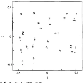
MUSIC estimates Results when SNR = 20dB 0.1

1

$2

s +

X X 0 X 0 + 6 x + + X 0 m + X X 0 + o+ X xx 0

*

o+ + ~ -0.1 0 5

Fig. 7 Results when SNR = lOdB 0 true source direction

x FNN estimates

+

MUSIC estimates -40

i

_-60 E 2 -80

s

g -100 -120 -140 -160

8

-180 .- c L 2 C c 0.1 . . . . . . _.! ...,... _. _. > ... . . . . . . . . . .. . . . . _. . ._. . . . ; ... : _.., ...,... _. _. ; ... .: ... : ... . . . . .. ; ... ... % . . . . . . . . . . ... ... 0 10 20 30 40 SNR Fig. 8 - FNN approach - - - MUSIC method True source direction at (0,O) 82

Root mean squares error against SNR

FNN to produce the estimates of the source direction. Meanwhile, the source direction is also estimated by the spatial smoothing 2-D MUSIC algorithm for comparison. The results are plotted in Fig. 5. We observe that the estimation error of the FNN-based estimator is satisfacto- rily small. This accuracy is a result of the universal function approximation capability of the FNNs. We also observe that the spatial smoothing 2-D MUSIC algorithm provides error-free estimates in the noise-free environment. We proceed to examine the estimation performance of these two algorithms in a noisy environment. Figs. 6 and 7 show the results when SNR=20dB, and lOdB, respectively. Clearly, the FNN is more robust to noise than the MUSIC algorithm.

To further investigate these two algorithms, we set the source direction at (0, 0) and make 100 independent Monte Carlo trials for various SNR values. The root mean square errors of these two algorithms are plotted in Fig. 8 as a function of SNR. We see that the FNN approach drastically outperforms the MUSIC algorithm for most SNR values.

0.1 U 0 -0.1 + + + + ++“ + + I I I I I -0.1 0 0.1 5 Fig. 9

True source direction at (0,O) x FNN estimates

+

MUSIC estimates Results when SNR = l2dB 0.1 U 0 -0.1 -0.1 +

*

+

++: +*+

:

&+JP

+++% + +%++ + + : + + * ++ +++ 0 5 0.1 Fig. 10

True source direction at (0,O)

x FNN estimates

+

MUSIC estimates

Results when SNR = 4dB

(6)

When SNR is higher than 34dB, the MUSIC algorithm performs better. This is a result of the limited approximation capability of the FNN. The limited approximation capability, however, is accurate enough. Figs. 9 and 10, are the results of all these 100 estimates when SNR= 12dB and 4dB, respectively. These figures tell us more about the performance improvement of the FNN approach over the spatial smoothing MUSIC approach.

6 Conclusions

The two dimensional direction finding problem in a multipath environment is studied and solved by a fuzzy neural network with an efficient reference-point preprocessing scheme. By computer simulations, we find that a small number of reference points is enough. The distances, calculated based on these reference points, possess enough information for estimating the direction of the radiating source. In the multipath environment, the FNN- based 2-D direction estimator substantially outperforms the spatial smoothing 2-D MUSIC algorithm, which is a high- resolution direction estimator. This may result from the poor decorrelation capability of the spatial smoothing scheme for close spacing signals. It may also result from the fact that the FNN-based estimator estimates only one direction while the MUSIC based algorithm has to estimate three directions using the same information. To sum up, for some complicated array signal processing problems, the artificial intelligence approach may be very helpful. In this paper, we have set up an example for this problem. Preprocessing is important when designing an artificial intelligence approach. Proper preprocessing reduces the complexity that the artificial intelligence mechanism should cope with, and preserves useful information as much as possible. The reference-point preprocessing

scheme proposed herein does this job very well for the 2-D direction finding problem.

7 1 2 3 4 5 6 7 8 9 References

SCHMIDT, R.O.: ‘Multiple emitter location and signal parameter estimation’, IEEE Antennas Propag. Mag., 1986, 34, pp. 276-380 ROY, R., and KAILATH, T.: ‘ESPRIT- Estimation of signal parameter via rotational invariance’, IEEE Trans. Acoust. Speech Signal Process., 1989,37, pp. 984-995

VIBERG, M., OTTERSTEN, B., and KAILATH, T.: ‘Sensor array processing based on subspace fitting’, IEEE Trans. Signal Process., 1991,39, pp. 2436-2448

STOICA, P., SHARMAN, K.C.: ‘Novel eigenanalysis method for direction estimation,’ IEE Proc., Radar Signal Process., 1990,137, pp 19-26 KUMMERT, A.: ‘Fuzzy technology implemented in sonar systems’, I E E E J Ocean. Eng., 1993, 18, pp. 4 8 3 4 9 0

MA, C.W., and TENG, C.C.: ‘Tracking a near-field moving target using h z z y neural networks’, Fuzzy Sets Syst. (to be published)

SOUTHALL, H.L., SIMMERS, J.A., and O’DONNELL, T.H.: ‘Direc- tion finding in phased arrays with a neural network beamformer’, IEEE Trans. Antennas Propag., 1995, 43, pp. 1369-1374

WONG, T., LO, T., LEUNG, H., LITVA, J., and BOSSE, E.: ‘Low angle radar tracking using radial basis function neural network’, IEE Proc., Radar Signal Process., 1993, 140, pp. 323-328

LO, T.K.Y., LEUNG, H., and LITVA, J.: ‘Artificial neural network for AOA estimation in a multipath environment over the sea’, IEEE 1

Ocean. E m . . 1994.19. uu. 555-562

10 LEUNG, fi.; LO, ’T., ’;id LITVA, J.: ‘Angle-of-arrival estimation in multipath environment using chaos theory’, Signal Process., 1993, 140, 11 ZOLTOWSKI, M., and HABER, E: ‘A vector space approach to direction finding in a coherent multipath environment’, IEEE Trans. Antennas Propag., 1986, AP-34, pp. 1069-1079

12 YUAN, Y.X., and SALT, J.E.: ‘Range and depth estimation using a vertical array in a correlated multipath environment’, IEEE 1 Ocean. Eng., 1993, 18, pp. 500-507

13 CHAO, C.T., CHEN, Y.J., and TENG, C.C.: ‘Simplification of fuzzy- neural systems using similarity analysis’, IEEE Trans. Syst. Man Cybern., 1996, 26, pp. 344-354

14 WANG, L.X.: ‘Adaptive fuzzy systems and control: design and stability analysis’ (Prentice Hall, Englewood Cliff, NJ, 1994

15 CHEN, Y.C., and TENG, C.C.: ‘A model reference control structure using a fuzzy neural network‘, F u z q Sets Syst., 1995, 73, pp. 291- 312

16 YEH, C.C., LEE, J.H., and CHEN, Y.M.: ‘Estimating two-dimensional angles of arrival in coherent source environment’, IEEE Trans. Acoust. Speech Signal Process. 1989,37, pp. 153-155

pp. 57-68