Maintenance of Association Rules in Data Mining

全文

(1)Maintenance of Association Rules in Data Mining Tzung-Pei Hong Department of Information Management I-Shou University Kaohsiung, 84008, Taiwan, R.O.C. tphong@isu.edu.tw. Ching-Yao Wang Institute of Computer and Information Science National Chiao Tung University Hsinchu, 300, Taiwan, R.O.C. cywang@cis.nctu.edu.tw. Abstract. upper support threshold to reduce the need for rescanning original databases and to save maintenance costs. The upper support threshold is the same as that used in conventional mining algorithms. The count of an itemset must be larger than the upper support threshold in order to be considered large. The lower support threshold defines the lowest count above which an itemset can be considered pre-large. In that algorithm, the lower support threshold is fixed and the number of new transactions allowed for not rescanning databases increases dynamically as databases grow. In this paper, we extend it and propose a new incrementally mining algorithm based on the upper and lower thresholds. The number of new transactions allowed for not rescanning databases is fixed, and the lower support threshold is dynamically close to the upper support threshold, making the additional overhead reduced in maintaining the consistency of association rules with the updated databases. The correctness of the algorithm is also proven.. In real-world applications, developing a mining algorithm that can incrementally maintain discovered information as a database grows is quite important. In the past, we proposed an incrementally mining algorithm that used a lower support threshold and an upper support threshold to reduce the need for rescanning original databases and to save maintenance costs. In this paper, we extend it and propose a new incrementally mining algorithm also based on the upper and lower thresholds. The number of new transactions allowed for not rescanning databases is fixed, and the lower support threshold is dynamically set close to the upper support threshold, making the additional overhead decreasing in maintaining the consistency of association rules with the updated databases. Keywords: data mining, association rule, large itemset, pre-large itemset, incremental mining.. 2. Review of the FUP Algorithm 1. Introduction Finding association rules [1-3][6][7][9][10-13] from transaction databases is most commonly seen in data mining. Conventional mining algorithms usually considers the database size static and focuses on batch mining. In real-world applications, however, new records are usually inserted into databases, and designing a mining algorithm that can maintain association rules as a database grows is thus critically important. Cheung and his co-workers proposed an incremental mining algorithm, called FUP (Fast UPdate algorithm) [4], for incrementally maintaining mined association rules and avoiding the shortcomings mentioned above. The FUP algorithm modifies the Apriori mining algorithm [2] and adopts the pruning techniques used in the DHP (Direct Hashing and Pruning) algorithm [10]. It first calculates large itemsets mainly from newly inserted transactions, and compares them with the previous large itemsets from the original database. According to the comparison results, FUP determines whether re-scanning the original database is needed, thus saving some time in maintaining the association rules. Hong et al. also proposed an incrementally mining algorithm [8] that used a lower support threshold and an. Cheung et al. proposed the FUP algorithm to incrementally maintain association rules when new transactions are inserted [4][5]. Using FUP, large itemsets with their counts in preceding runs are recorded for later use in maintenance. As new transactions are added, FUP first scans them to generate candidate 1-itemsets (only for these transactions), and then compares these itemsets with the previous ones. FUP partitions candidate 1-itemsets into two parts according to whether they are large for the original database. If a candidate 1-itemset from the newly inserted transactions is also among the large 1-itemsets from the original database, its new total count for the entire updated database can easily be calculated from its current count and previous count since all previous large itemsets with their counts are kept by FUP. Whether an original large itemset is still large after new transactions are inserted is determined from its support ratio as its total count over the total number of transactions. By contrast, if a candidate 1-itemset from the newly inserted transactions does not exist among the large 1-itemsets in the original database, one of two possibilities arises. If this candidate 1-itemset is not large for the new transactions, then it cannot be large for the entire updated database, which means no action is necessary. If this candidate 1-itemset is.

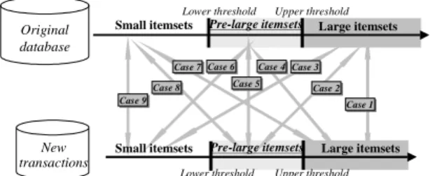
(2) large for the new transactions but not among the original large 1-itemsets, the original database must be re-scanned to determine whether the itemset is actually large for the entire updated database. Using the processing tactics mentioned above, FUP is thus able to find all large 1-itemsets for the entire updated database. After that, candidate 2-itemsets from the newly inserted transactions are formed and the same procedure is used to find all large 2-itemsets. This procedure is repeated until all large itemsets have been found.. In [8], we propose the concept of pre-large itemsets. A pre-large itemset is not truly large, but promises to be large in the future. A lower support threshold and an upper support threshold are used to realize this concept. The upper support threshold is the same as that used in the conventional mining algorithms. The support ratio of an itemset must be larger than the upper support threshold in order to be considered large. On the other hand, the lower support threshold defines the lowest support ratio for an itemset to be treated as pre-large. Pre-large itemsets act like buffers in the incremental mining process and are used to reduce the movements of itemsets directly from large to small and vice-versa. Considering an original database and transactions newly inserted using the two support thresholds, itemsets may thus fall into one of the following nine cases (illustrated in Figure 1). Lower threshold. Small itemsets. Upper threshold. Pre-large itemsets. Case Case 66 Case 77 Case Case Case 88. Large itemsets. Case Case 44 Case Case 33. Case Case 55. Case Case 22. Case Case 99. New transactions. Case Case 11. Small itemsets. LTk : the set of large k-itemsets from T;. LUk : the set of large k-itemsets from U; PkD : the set of pre-large k-itemsets from D;. 3. Pre-large Itemsets. Original database. U : the entire updated database, i.e., D∪ T; d : the number of transactions in D; n : the number of transactions in T; Sl : the lower support threshold for pre-large itemsets; Su : the upper support threshold for large itemsets, Su >Sl; D Lk : the set of large k-itemsets from D;. Pre-large itemsets. Lower threshold. Large itemsets. Upper threshold. Figure 1: Nine cases arising from adding new transactions to existing databases Cases 1, 5, 6, 8 and 9 above will not affect the final association rules. Cases 2 and 3 may remove existing association rules, and cases 4 and 7 may add new association rules. If we retain all large and pre-large itemsets with their counts after each pass, then cases 2, 3 and case 4 can be handled easily. Also, in the maintenance phase, the ratio of new transactions to old transactions is usually very small. This is more apparent when the database is growing larger. An itemset in case 7 cannot possibly be large for the entire updated database as long as the number of transactions is small compared to the number of transactions in the original database.. 4. Notation The notation used in this paper is defined below. D : the original database; T : the set of new transactions;. PkT : the set of pre-large k-itemsets from T; PkU : the set of pre-large k-itemsets from U; Ck : the set of all candidate k-itemsets from T; I : an itemset; SD(I) : the count of I in D; ST(I) : the count of I in T; SU(I) : the count of I in U.. 5. Theoretical Foundation As mentioned above, if the number of new transactions is small compared to the number of transactions in the original database, an itemset that is small (neither large nor pre-large) in the original database but is large in the newly inserted transactions cannot possibly be large for the entire updated database. In the maintaining phase of databases on real applications, the numbers of new inserted transactions are usually small compared to the sizes of the entire databases. Lower support thresholds can thus be set close to upper support thresholds. This is proven in the following theorem. Theorem 1: let Sl and Su be respectively the lower and the upper support thresholds, and let d and t be respectively the numbers of the original and new transactions. If Sl ≤ Su −. t (1 − Su ) , then an itemset that d. is small (neither large nor pre-large) in the original database but is large in newly inserted transactions is not large for the entire updated database. Proof: The following derivation can be obtained from Sl ≤ Su − t (1 − Su ) : d Sl ≤ Su −. t (1 − Su ) d. ⇒. t(1-Su) ≤ (Su- Sl) d. ⇒. t-tSu ≤ dSu- dSl. ⇒. t+ dSl ≤ Su(d+t). ⇒. t + dSl ≤ S . u d +t. (1). If an itemset I is small (neither large nor pre-large) in the original database D, then its count SD(I) must be less than Sl∗d, therefore,.

(3) SD(I) < dSl. If I is large in the newly inserted transactions T, then: t ≥ ST(I) ≥ tSu. The entire support ratio of I in the updated database U U is S ( I ) , which can be further expanded to: d +t S U (I ) S T (I ) + S D (I ) = d +t d +t < <. t + dSl d +t S u.. I is thus not large for the entire updated database. This completes the proof. Example 1: Assume D=100, t=10 and Su=60%. An appropriate Sl can be derived as follows: Sl = Su −. t (1 − Su ) =0.6 - 0.1(1-0.6)=0.56. d. Thus, if the lower support threshold is equal to or less than 0.56, then I is absolutely not large for the entire updated database. From theorem 1, the lower support threshold required for efficient handling of case 7 is determined by Su, t, and d. It can easily be seen from Formula 1 that if d grows larger, then Sl will be larger too. Therefore, as the database grows, the overhead of our proposed approach becomes small. This characteristic is especially useful for real-world applications. As more new transactions are added to the original database, Sl can thus be set at a higher value. The following corollary can thus be achieved. It proof is omitted here. Corollary 1: Assume the number t of newly inserted old transactions is fixed each time. If S lnew = S old + t ( Su − Sl ) , l d old + t then an itemset which is small (neither large nor pre-large) for the lower support threshold S lold before t new transactions are inserted into the database but is large in the newly inserted transactions, is not large for the lower support threshold S lnew after t new transactions are inserted into the database.. 6. The maintenance algorithm based on dynamic lower support thresholds According to the discussion above, an efficient maintenance algorithm can be designed for incrementally inserted transactions. The large and pre-large itemsets with their counts in preceding runs are recorded for later use in maintenance. As new transactions are added, the proposed algorithm first scans them to generate candidate 1-itemsets (only for these transactions), and then. compares these itemsets with the previously retained large and pre-large 1-itemsets. It partitions candidate 1-itemsets into three parts according to whether they are large or pre-large for the original database. If a candidate 1-itemset from the newly inserted transactions is also among the large or pre-large 1-itemsets from the original database, its new total count for the entire updated database can easily be calculated from its current count and previous count since all previous large and pre-large itemsets with their counts have been retained. Whether an originally large or pre-large itemset is still large or pre-large after new transactions have been inserted is determined from its new support ratio, as derived from its total count over the total number of transactions. On the contrary, if a candidate 1-itemset from the newly inserted transactions does not exist among the large or pre-large 1-itemsets in the original database, then it is absolutely not large for the entire updated database as long as the number of newly inserted transactions is within the predefined number of new transactions. In this situation, no action is needed. When transactions are incrementally added and the total number of new transactions exceeds the predefined threshold, the original database is re-scanned to find new pre-large itemsets for a new lower support threshold. The proposed algorithm can thus find all large 1-itemsets for the entire updated database. After that, candidate 2-itemsets from the newly inserted transactions are formed and the same procedure is used to find all large 2-itemsets. This procedure is repeated until all large itemsets have been found. The details of the proposed maintenance algorithm are described below. A variable, c, is used to record the number of new transactions since the last re-scan of the original database. The proposed maintenance algorithm: INPUT: A predefined upper support threshold Su and new transaction number threshold t, a set of large itemsets and pre-large itemsets in the original database consisting of (d+c) transactions, a set of n new transactions, and a dynamic lower support threshold Slold , which is S lold = Su − t (1 − Su ) . d   OUTPUT: A set of final association rules for the updated database. STEP 1: If c+n ≥ t, set: S lnew = S lold +. t ( Su − S lold ) , d + (c + n ). Otherwise, set S lnew = S lold . STEP 2: Set k =1, where k records the number of items in itemsets currently being processed. STEP 3: Find all candidate k-itemsets Ck and their counts from the new transactions. STEP 4: Divide the candidate k-itemsets into three parts according to whether they are large or pre-large in the original database. STEP 5: For each itemset I in the originally large.

(4) k-itemsets LDk , do the following substeps: Substep 5-1: Set the new count SU(I) = ST(I)+ SD(I). Substep 5-2: If SU(I)/(d+c+n) ≥ Su, then assign I as a large itemset, set SD(I) = SU(I) and keep I with SD(I), Otherwise, if SU(I)/(d+c+n) ≥ S lnew , then assign I as a pre-large itemset, set SD(I) = SU(I) and keep I with SD(I), Otherwise, neglect I.. Table 1: An original database with TID and Items Incremental database TID Items 100 ACD 200 BCE 300 ABCE 400 ABE 500 ABE 600 ACD 700 BCDE 800 BCE. STEP 6: For each itemset I in the originally pr-large itemset PkD , do the following substeps: Substep 6-1: Set the new count SU(I) = ST(I)+ SD(I). Substep 6-2: If SU(I)/(d+c+n) ≥ Su, then assign I as a large itemset, set SD(I) = SU(I) and keep I with SD(I), Otherwise, if SU(I)/(d+c+n) ≥ S lnew , then assign I as a pre-large itemset, set SD(I) = SU(I) and keep I with SD(I), Otherwise, neglect I. STEP 7: For each itemset I in the candidate itemsets that is not in the originally large itemsets LD k or pre-large itemsets. PkD , do the following. substeps: Substep 7-1: If I is in the large itemsets LTk or pre-large itemsets PkT from the new transactions, then put it in the rescan-set R. Substep 7-2: If I is small for the new transactions, then do nothing. STEP 8: If c+n < t or R is null, then do nothing, else rescan the original database to determine whether the itemsets in the rescan-set R are large or pre-large. STEP 9: Form candidate (k+1)-itemsets Ck+1 from finally large and pre-large k-itemsets ( LUk U PkU ) that appear in the new transactions. STEP 10: Set k = k+1. STEP 11: Repeat STEPs 4 to 10 until no new large or pre-large itemsets are found. STEP 12: Modify the association rules according to the modified large itemsets. STEP 13: If c+n ≥ t, then set d=d+c+n, c=0 and S lold = S lnew ; otherwise, set c=c+n.. Also assume the predefined upper support threshold Su is set at 50%, the new transaction threshold t is set at 2, the current old lower support S lold is 37.5%, which is calculated as:  . Slold =  Su −. t 2    (1 − Su )  = 0.5 − (1 − 0.5) = 0.375 = 37.5% . d 8   . Moreover, the sets of large itemsets and pre-large itemsets for the given initial data are shown in Tables 2 and 3. Table 2: The large itemsets for the original database Large itemsets 1 item Count 2 items Count 3 items A 5 BC 4 BCE B 6 BE 6 C 6 CE 4 E 6. Count 4. Table 3: The pre-large itemsets for the original database Pre-large itemsets 1 item Count 2 items Count 3 items Count D 3 AB 3 ABE 3 AC 3 AE 3 CD 3. Assume one new transaction is inserted into the data set with TID=900, Items={A,B,D,F}. The variable c is initially set at 0. The proposed incremental mining algorithm proceeds as follows. STEP 1: Since c+n(=0+1)<t(=2), set S lnew =0.375.. After Step 13, the final association rules for the updated database can then be found.. STEP 2: k is set to 1, where k records the number of items in itemsets currently being processed.. 7. An example. STEP 3: All candidate 1-itemsets C1 and their counts from the new transaction are found, as shown in Table 4.. In this section, an example is given to illustrate the proposed incremental data-mining algorithm. Assume the initial data set includes 8 transactions, which are shown in Table 1..

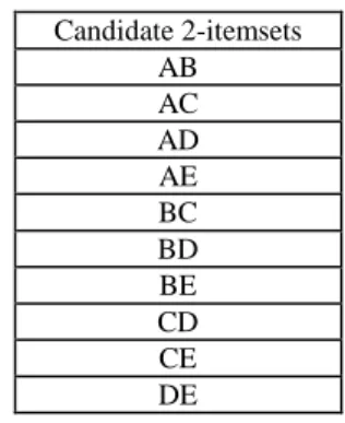
(5) Table 4: All candidate 1-itemsets for the new transaction Candidate 1-itemsets Items Count A 1 B 1 D 1 F 1. STEP 4: From Table 4, all candidate 1-itmesets {A}{B} {D}{F} are divided into three parts, {A}{B}, {D}, and {F} according to whether they are large or pre-large in the original database. Results are shown in Table 5.. transactions, it is put in the rescan-set R. STEP 8: Since c+n(=0+1) < t(=2), rescanning the database is unnecessary, so nothing is done. STEP 9: From Steps 5,6 and 7, the final large 1-itemsets and pre-large 1-itemsets for the updated database are {A}, {B}, {C}, {D} and {E}. All candidate 2-itemsets generated from them are shown in Table 7. Table 7: All candidate 2-itemsets for the new transactions Candidate 2-itemsets AB AC AD AE BC BD BE CD CE DE. Table 5: Three partitions of all candidate 1-itemsets from the new transaction Pre-large Neither Large Large 1-Itemsets 1-Itemsets for Nor Pre-large for the initial the initial data 1-itemsets for the data set initial Data set set Items Count Items Count Items Count A 1 D 1 F 1 B 1. STEP 5: The following substeps are done for each of the originally large 1-itemsets {A}, {B}, {C} and {E}: Substep 5-1: The final counts of the candidate 1-itemsets {A}, {B}, {C} and {E} are calculated using ST(I)+ SD(I). Table 6 shows the results. Table 6: The final counts of {A}, {B}, {C} and {E} Items A B C E. Count 6 7 6 6. Substep 5-2: The new support ratios of {A}, {B}, {C} and {E} are calculated. For example, the new support ratio of {A} is 6/(8+1) ≥ 0.5. {A} is thus still a large itemset. In this example, {A}, {B}, {C} and {E} are all large and retained in the large 1-itemsets with their new counts for the updated database. STEP 6: The following substeps are done for itemset {D}, which is originally pre-large: Substep 6-1: The final count of the candidate 1-itemset {D} is calculated using ST(I)+ SD(I) (= 4). Substep 6-2: The new support ratio of {D} is 4/(8+1) > 0.375 but <0.5, {D} is thus a pre-large 1-itemset for the updated database. {D} with its new count is retained in the set of pre-large 1-itemsets for the updated database. STEP 7: Since the itemset {F}, which was originally neither large nor pre-large, is large for the new. STEP 10: k = k+1=2. STEP 11: Steps 4 to 10 are repeated to find large or pre-large 2-itemsets. Results are shown in Table 8. Table 8: All large 2-itemsets and pre-large 2-itemsets for the updated database Large 2-Itemsets Items BE. Count 6. Pre-large 2-Itemsets Items AB BC CE. Count 4 4 4. Large or pre-large 3-itemsets are found in the same way. No large 3-itemsets were found in this example. STEP 12: The association rules derived from the newly found large itemsets are: B⇒E (Confidence=6/7), and E⇒B (Confidence=6/7). STEP 13: Since c+n(=0+1)<t(=2), c=c+n=0+1=1.. 8. Conclusions In this paper, we have extended our previous method and proposed a new incrementally mining algorithm based on the concept of pre-large itemsets. The pre-large itemsets act as a gap to avoid small itemsets becoming large in the updated database when transactions are inserted. The number of new transactions allowed for not rescanning databases is fixed, and the lower support threshold is dynamically set close to the upper support threshold, making the additional overhead decreasing in maintaining the consistency of association rules with the updated databases. If the size of the database grows larger,.

(6) then the lower support threshold will be larger too. Therefore, as the database grows, our proposed approach becomes increasingly efficient. This characteristic is especially useful for real-world applications. References [1] R. Agrawal, T. Imielinksi and A. Swami, “Mining association rules between sets of items in large database,“ The ACM SIGMOD Conference, Washington DC, USA, 1993 [2] R. Agrawal and R. Srikant, “Fast algorithm for mining association rules,” The International Conference on Very Large Data Bases, pp. 487-499, 1994. [3] R. Agrawal, R. Srikant and Q. Vu, “Mining association rules with item constraints,” The 3th International Conference on Knowledge Discovery in Databases and Data Mining, Newport Beach, California, 1997. [4] D. W. Cheung, J. Han, V. T. Ng, and C. Y. Wong, “Maintenance of discovered association rules in large databases: An incremental updating approach,” The 12th IEEE International Conference on Data Engineering, 1996. [5] D. W. Cheung, S. D. Lee, and B. Kao, “A general incremental technique for maintaining discovered association rules,” The 5th International Conference On Database Systems For Advanced Applications (DASFAA), Melbourne, Australia, pp. 185-194, 1997. [6] T. Fukuda, Y. Morimoto, S. Morishita and T. Tokuyama, "Mining optimized association rules for numeric attributes,". The ACM SIGACT-SIGMOD-SIGART Symposium on Principles of Database Systems, pp. 182-191, 1996 [7] J. Han and Y. Fu, “Discovery of multiple-level association rules from large database,” The 21th International Conference on Very Large Data Bases, Zurich, Swizerland, pp. 420-431, 1995. [8] T. P. Hong, C. Y. Wang and Y. H. Tao, "Incremental data mining based on two support thresholds," submitted to The 11th National Conference on Artificial Intelligence (AAAI), 2000. [9] H. Mannila, H. Toivonen and A. I. Verkamo, “Efficient algorithm for discovering association rules,” The AAAI Workshop on Knowledge Discovery in Databases, pp. 181-192, 1994. [10] J. S. Park; M. S. Chen and P. S. Yu, “Using a hash-based method with transaction trimming for mining association rules,” IEEE Transactions on Knowledge and Data Engineering, Vol. 9, No. 5, pp.812-825, 1997. [11] N. L. Sarda and N. V. Srinivas, “An adaptive algorithm for incremental mining of association rules,” The 9th International Workshop on Database and Expert Systems, 1998. [12] R. Srikant and R. Agrawal, “Mining generalized association rules,” The 21th International Conference on Very Large Data Bases, Zurich, Swizerland, pp. 407-419, 1995. [13] R. Srikant and R. Agrawal, “Mining quantitative association rules in large relational tables,” The ACM SIGMOD International Conference on Management of Data, Monreal, Canada, June, pp. 1-12, 1996..

(7)