多輸入多輸出正交分頻多工通信之通道估測技術研究

全文

(1)國立交通大學電子工程學系電子研究所碩士班碩士論文. 多輸入多輸出正交分頻多工通信之通道估測技術研究 On Channel Estimations for MIMO OFDM Systems. 研究生：詹偉廷指導教授：陳紹基博士. 中華民國九十四年八月.

(2) 多輸入多輸出正交分頻多工通信之通道估測技術研究 On Channel Estimations for MIMO OFDM Systems 研究生：詹偉廷. Student：Wei-Ting Chan. 指導教授：陳紹基博士. Advisor：Sau-Gee Chen. 國立交通大學電子工程學系. 電子研究所所碩士班. 碩士論文. A Thesis Submitted to Department of Electronics Engineering & Institute of Electronics College of Electrical Engineering and Computer Science National Chiao Tung University in Partial Fulfillment of the Requirements for the Degree of Master in Electronics Engineering. August 2005 Hsinchu, Taiwan, Republic of China. 中華民國九十四年八月.

(3) 多輸入多輸出正交分頻多工通信之通道估測技術研究. 學生: 詹偉廷. 指導老師: 陳紹基博士. 國立交通大學. 電子工程學系電子研究所碩士班. 摘. 要. 在本篇論文中探討了數種多輸入多輸出正交多工分頻系統中的通道估測技術。我們所主要討論的系統平台包含採用梳狀式(comb-type)傳輸的 802.16a 時空碼模式以及採用區塊式(block-type)傳輸的 802.11n-like 系統，並且配合不同引導訊號的使用。以採分散式(scattered)導引訊號的 802.11n-like 系統來說，我們主要討論內插技巧對這個系統的影響。為了克服非整數取樣空間通道的問題，我們嚐試了離散式餘弦轉換式內插法。模擬結果證實在此系統中較採用傳統離散式傅立葉轉換有所改善。而在含有時空碼先導訊號的 802.11n-like 系統中，我們利用通道追蹤(tracking)的技巧來改善在時變通道下的效能。在討論使用全引導訊號式(all-pilot preamble)的 MIMO 系統時，我們也討論基於最小平方差的估測技巧，並為現有的簡化作法提出一個簡單的通道長度估測法。我們利用 WWiSE 提案的系統進行全引導訊號式系統的模擬，證實了此一方法適合在 WWiSE 的標準下中使用。至於對具有時空碼結構的梳狀式傳輸系統，我們則以含有時空碼的 802.16a 系統作為模擬平台，評估各種內插方式的效能。 I.

(4) On Channel Estimations for MIMO OFDM Systems Student: Chan Wei-Ting. Advisor: Dr. Chen Sau-Gee. Department of Electronics Engineering & Institute of Electronics National Chiao Tung University. ABSTRACT In this thesis, several schemes for channel estimation for MIMO OFDM systems are investigated. Both 802.16a with STC (comb-type) and 802.11n-like systems (block-type) are explored in our studies. For scattered preamble in 802.11n-like systems, different interpolation skills are evaluated. To overcome the effect of non-sample spaced channel, DCT-based interpolation is tried. The simulation results show that it is better than DFT-based estimator in this MIMO system. For STBC preamble in 802.11n-like systems, a channel tracking skill is used to improve its performance under time-varying channel. For all-pilot preamble in 802.11n-like systems, a LS-based estimation method is studied. A simple method to detect the length of channel is proposed for this method. With WWiSE standard, this estimation method is evaluated and shown to be suitable for this standard. Also, estimation schemes for comb-type MIMO OFDM systems are also explored in thesis. We evaluate the performances of interpolation techniques applied to 802.16a system with STC. II.

(5) 致謝. 完成這份碩士學位論文後，不可免俗的要向諸位對我助益良多的師長朋友表達感謝之意。首先最重要的，我必須感謝我的指導教授陳紹基老師。在兩年內，老師在研究方法，專業探討，以及處事態度上給我許多建言，在此深深向老師致謝。作論文的這段時間內，實驗室同學承穎，世民給了我許多有形無形的幫助；佳旻，元志和觀易在口試前的這段時間給了我很多建議以及協助，並且在論文的用詞遣字字上提供建言；另外感謝特別曲建全學長兩年來的照顧，教導我許多研究以外的事情。雅娣在這段時間中除了在寫作上給予很多專業建議外，在我陷入低潮的時候也花許多時間為我分擔煩惱，是這段忙碌時期的一盞引路燈。我也要感謝我的家人，除了讓我在物質生活上不需煩憂，能夠專心求學外，也時常給我很多必要的建言。更重要的是感謝父母給予我生命以及心靈，使我有機會體驗這個世界的驚喜。. 我算不上是一個創造論者，但倘若這充滿難解矛盾以及神秘美感的世界真是由造物主所創生的，在此對其致上謝意。. III.

(6) Content Content....................................................................................................................... IV List of Tables ............................................................................................................. VI List of Figures...........................................................................................................VII Chapter 1 Introduction................................................................................................1 Chapter 2 Fundamentals of MIMO OFDM Systems ...............................................3 2.1 OFDM System Model......................................................................................3 2.1.1 Continuous and Discrete-Time Models of OFDM Systems .................4 2.1.2 The Concept of Guard Interval and Cyclic Prefix ................................6 2.1.3 The Properties of Transmission Channels in Wireless Communication ........................................................................................................................8 2.2 Studies and Simulations of MIMO Channels ..................................................9 2.2.1 Wireless MIMO Channel Simulators..................................................10 2.2.2 Studies and Simulation Results...........................................................14 Chapter 3 Standards of IEEE 802.11n (WWiSE) and IEEE 802.16a ................19 3.1 IEEE 802.16a standard...................................................................................19 3.1.1 802.16a OFDMA Frame and Symbol Structures................................21 3.1.2 802.16a OFDMA Carrier Allocation ..................................................23 3.1.3 802.16a OFDMA Space-Time Coding (STC) ....................................26 3.2 IEEE 802.11n WWiSE Proposal....................................................................27 3.2.1 Physical Layer Parameters of WWiSE ...............................................28 3.2.2 Frame Structure of WWiSE Mandatory Mode ...................................29 3.2.3 The Code Structure of Space-time Block Code..................................31 Chapter 4. Channel Estimations for MIMO OFDM Systems .............................33. 4.1 Preamble Design for MIMO OFDM Systems ...............................................33 4.1.1 Scattered Preamble..............................................................................34 4.1.2 Space-time Coded Preamble ...............................................................35 IV.

(7) 4.1.3 All-pilot Preambles .............................................................................37 4.2 Channel Estimation Techniques for MIMO OFDM System .........................38 4.2.1 Channel Estimation for Scattered Preambles......................................38 4.2.1.1 Piecewise Linear Interpolation ................................................39 4.2.1.2 SPLINE Interpolation ..............................................................40 4.2.1.3 Transform-Domain Interpolation.............................................41 4.2.2 Channel Estimation for Space-time Coded Preamble.........................51 4.2.2.1 Decision-direct Channel Tracking for Space-time Coded Preamble ..............................................................................................53 4.2.3 Channel Estimation with All-pilot Preamble......................................55 4.2.3.1 Complexity Analysis of LS Channel Estimator for MIMO OFDM System Using All-pilot Preambles ..........................................58 4.2.3.2 Proposed Method for the Decision of Significant Number of Channel Taps .......................................................................................60 Chapter 5 Simulations and Comparisons .............................................................63 5.1 Simulation Environment and Parameters.......................................................63 5.1.1 Channel Models ..................................................................................64 5.2 Channel Estimation for 802.11n-like Systems...............................................66 5.2.1 Channel Estimation for Space-Time Coded Preamble MIMO OFDM ......................................................................................................................67 5.2.2 Channel Estimation for All-pilot Preamble MIMO OFDM ...............70 5.2.3 Channel Estimation for MIMO OFDM Systems with Scattered Preamble ......................................................................................................87 5.3 Channel Estimation for 802.16a OFDMA with STC.....................................91 5.3.1 Pilot Sample Grouping for 2-D Channel Estimations.........................93 5.3.2 Non-sample Spaced Effect in 802.16a STC System.........................100 Chapter 6 Conclusion ..............................................................................................102 Bibliography .............................................................................................................104 Autobiography..........................................................................................................107. V.

(8) List of Tables TABLE 2.1 DESIRED SPATIAL CORRELATION MATRIX OF THE CHANNEL SIMULATOR ................................. 16 TABLE 2.2 RESULTING SPATIAL CORRELATION MATRIX OF THE CHANNEL SIMULATOR ................................ 17 TABLE 3.1 MAIN BASEBAND FEATURES OF 802.16A-2003............................................................................ 21 TABLE 3.2 DETAILED CARRIER ALLOCATION OF DL 802.16A OFDMA [11] ............................................. 25 TABLE 3.3 ENCODING PATTERN OF 802.16A STC MODE ............................................................................... 26 TABLE 3.4 MAIN FEATURES OF WWISE BASEBAND MANDATORY MODE .................................................. 28 TABLE 4.1 TRAINING SYMBOL ARRANGEMENT OF SPACE-TIME CODED PREAMBLE .................................... 36 TABLE 4.2 CHANNEL PARAMETERS FOR INDOOR WIRELESS CHANNEL (MODEL 1) ..................................... 43 TABLE 4.3 CHANNEL PARAMETERS FOR INDOOR WIRELESS CHANNEL (MODEL 2) ..................................... 43 TABLE 4.4 COMPUTATIONAL COMPLEXITY OF MATRIX INVERSION WITH GAUSSIAN ELIMINATION ( N0. ≡ NT × K 0 )................................................................................................................................... 59. TABLE 5.1 SIMULATED 802.11N-LIKE MIMO SYSTEM PARAMETERS .......................................................... 64 TABLE 5.2 STATIC PARAMETERS FOR INDOOR WIRELESS CHANNEL (MODEL 1).......................................... 65 TABLE 5.3 STATIC PARAMETERS FOR INDOOR WIRELESS CHANNEL (MODEL 2).......................................... 65 TABLE 5.4 STATIC PARAMETERS FOR ETSI MODEL A (MODEL 3)................................................................ 65 TABLE 5.5 STATIC PARAMETERS FOR ATTC MODEL E (MODEL 4) .............................................................. 66 TABLE 5.6 SIMULATION PARAMETERS OF 802.16A STC SYSTEM (2 X 1)..................................................... 92. VI.

(9) List of Figures FIGURE 2.1(A) CONTINUOUS MODEL OF OFDM MODULATOR ........................................................................ 4 FIGURE 2.1(B) CONTINUOUS MODEL OF OFDM DEMODULATOR.................................................................... 5 FIGURE 2.2 SPECTRUM OF A SINGLE OFDM SYMBOL ...................................................................................... 5 FIGURE 2.3 DISCRETE SYSTEM MODEL OF OFDM SYSTEM ............................................................................. 6 FIGURE 2.4 INTER-SYMBOL-INTERFERENCE OF WIRELESS PROPAGATION ...................................................... 7 FIGURE 2.5 CYCLIC PREFIX OF AN OFDM SYMBOL ......................................................................................... 7 FIGURE 2.6 SIMULATOR STRUCTURE DIAGRAM FOR GENERATING SPATIAL CORRELATED FADING MODEL (A) SIMULATOR FLOW DIAGRAM (B) SIGNAL FLOW DIAGRAM ................................................................... 14. FIGURE 2.7 SIMULATION FLOW OF THE ADOPTED MIMO CHANNEL SIMULATOR ....................................... 14 FIGURE 2.8 MAGNITUDE DISTRIBUTION OF FOUR CORRELATED FADING CHANNELS .................................. 15 FIGURE 2.9 PHASE DISTRIBUTION OF FOUR CORRELATED FADING CHANNELS (POLAR PLOT) .................... 16 FIGURE 3.1 FRAME STRUCTURE OF 802.16A OFDMA [11]........................................................................... 22 FIGURE 3.2 TIME-DOMAIN STRUCTURE OF A 802.16A SYMBOL .................................................................... 22 FIGURE 3.3 802.16A SYMBOL FREQUENCY DOMAIN STRUCTURE .................................................................. 23 FIGURE 3.4 CARRIER ALLOCATION OF DL 802.16A OFDMA [11] .............................................................. 25 FIGURE 3.5 TX/RX ARCHITECTURE OF 802.16A WITH STC [11] ................................................................... 27 FIGURE 3.6 TRANSMITTER SYMBOL ARRANGEMENT OF 802.16A STC [11]................................................. 27 FIGURE 3.7 FRAME STRUCTURE OF WWISE 802.11N PROPOSAL [13] ......................................................... 29 FIGURE 3.8 DETAILED FRAME STRUCTURE OF 802.11N SYSTEM [13]........................................................... 30 FIGURE 3.9 FRAME STRUCTURE OF WWISE SYSTEM WITH TWO TRANSMISSION ANTENNAS [12]............. 30 FIGURE 3.10 FRAME STRUCTURE OF SYSTEM WWISE WITH FOUR TRANSMISSION ANTENNAS [12] ......... 31 FIGURE 4.1 CLASSIFICATION OF PILOT ARRANGEMENT IN MIMO OFDM .................................................. 34 FIGURE 4.2 FRAME STRUCTURE OF A 2X1 MIMO OFDM SYSTEM WITH SCATTERED PILOT...................... 35 FIGURE 4.3 RECEIVING AND DECODING STRUCTURE OF A 2X1 SPACE-TIME CODED SYSTEM ..................... 36 VII.

(10) FIGURE 4.4 FRAME STRUCTURE A 2X1 MIMO OFDM SYSTEM WITH SPACE TIME CODED PILOT .............. 37 FIGURE 4.5 ILLUSTRATION OF CHANNEL SEGMENTATION AND THE REQUIRED KNOWN PARAMETERS FOR CUBIC SPLINE INTERPOLATION ............................................................................................................... 40. FIGURE 4.6 REGULAR PILOT PLACEMENT........................................................................................................ 41 FIGURE 4.7 CONTINUOUS AND DISCRETE IMPULSE RESPONSES OF INDOOR MODEL 1 ................................. 45 FIGURE 4.8 CONTINUOUS AND DISCRETE IMPULSE RESPONSES OF INDOOR MODEL 2 ................................. 45 FIGURE4.9 MAGNITUDE PLOT OF TAP WEIGHT OF NON-SAMPLE SPACED CHANNEL .................................... 46 FIGURE 4.10 DFT-BASED CHANNEL ESTIMATOR ............................................................................................ 48 FIGURE 4.11 IDCT/DCT-BASED CHANNEL ESTIMATOR ................................................................................ 50 FIGURE 4.12 EQUIVALENT CHANNEL ESTIMATORS BY IDCT/DCT-BASED INTERPOLATOR AND IDFT-BASED INTERPOLATOR ................................................................................................................. 51 FIGURE 4.13 ILLUSTRATION OF RECEIVED STBC SYMBOL ........................................................................... 53 FIGURE 4.14 FUNCTION STRUCTURE OF LS CHANNEL ESTIMATION FOR MIMO OFDM SYSTEMS USING ALL-PILOT PREAMBLES ........................................................................................................................... 58. FIGURE 4.15 CRITERIA FOR LENGTH OF THE ESTIMATED CHANNEL.............................................................. 61 FIGURE 4.16 FLOW CHART FOR PROPOSED CHANNEL LENGTH DETECTION ALGORITHM............................. 62 FIGURE 5.1 BER COMPARISON OF SPACE-TIME CODED PREAMBLE SYSTEM (2 X 1) FOR TWO DIFFERENT CHANNEL CONDITIONS (A) MODEL 1 (B) MODEL 2 .............................................................................. 68. FIGURE 5.2 BER COMPARISON OF SPACE-TIME CODED PREAMBLE SYSTEM WITH DECISION-DIRECT TRACKING (2 X 1) FOR TWO DIFFERENT CHANNEL CONDITIONS (A) MODEL 1 (B) MODEL 2............ 69. FIGURE 5.3 RESPONSE PLOT OF SPACE-TIME CODED PREAMBLE SYSTEM WITH DECISION-DIRECT TRACKING (2 X 1) FOR THE FIRST SYMBOL AND THE LAST SYMBOL IN A PACKET ................................................ 70 FIGURE 5.4 ESTIMATED CHANNEL RESPONSES FOR THREE DIFFERENT. K 0 (A) K 0 =15 (B) K 0 =7 (C). K 0 =4 ...................................................................................................................................................... 72. VIII.

(11) FIGURE 5.5 AVERAGED MSE VERSUS. K0. OF AN ALL-PILOT PREAMBLE SYSTEM, NT=2, ASSUMED A. STATIC TWO-RAY MODEL ....................................................................................................................... 73. FIGURE 5.6 BER COMPARISON DUE TO VARIOUS. K0. VALUES, ALL-PILOT-PREAMBLE, WITH NT=2, NR =1,. ASSUMED A STATIC TWO-RAY MODEL ................................................................................................... 74. FIGURE 5.7 BER COMPARISON DUE TO VARIOUS. K0. VALUES, ALL-PILOT-PREAMBLE, WITH NT=2, NR. =1(A) MODEL 1 (B) MODEL 2 ................................................................................................................ 76 FIGURE 5.8 BER COMPARISON DUE TO VARIOUS. K0. VALUES, ALL-PILOT-PREAMBLE, WITH NT=3, NR =1. (A) MODEL 1 (B) MODEL 2..................................................................................................................... 77 FIGURE 5.9 BER COMPARISON DUE TO VARIOUS. K0. VALUES, ALL-PILOT-PREAMBLE, WITH NT=4, NR =1. (A) MODEL 1 (B) MODEL 2..................................................................................................................... 78 FIGURE 5.10 BER COMPARISON DUE TO VARIOUS. K0. VALUES, ALL-PILOT-PREAMBLE, NT=2, NR =2. (MODEL 1) ............................................................................................................................................... 79 FIGURE 5.11 BER COMPARISON DUE TO VARIOUS. K0. VALUES, ALL-PILOT-PREAMBLE, NT=3, NR =3. (MODEL 1) ............................................................................................................................................... 80 FIGURE 5.12 BER COMPARISON DUE TO VARIOUS. K0. VALUES, ALL-PILOT-PREAMBLE, NT=4, NR =4. (MODEL 1) ............................................................................................................................................... 80 FIGURE 5.13 AVERAGED MSE VERSUS. K0. OF ALL-PILOT PREAMBLE SYSTEM, NT=2 (A) MODEL 1 (B). MODEL 2.................................................................................................................................................. 81 FIGURE 5.14 AVERAGED MSE VERSUS. K0. OF ALL-PILOT PREAMBLE SYSTEM, NT=3 (A) MODEL 1 (B). MODEL 2.................................................................................................................................................. 82 FIGURE 5.15 AVERAGED MSE VERSUS. K0. OF ALL-PILOT PREAMBLE SYSTEM, WITH NT=4 (A) MODEL 1 (B). MODEL 2.................................................................................................................................................. 83 IX.

(12) FIGURE 5.16 MSE AND. K0. CURVES VERSUS ITERATION NO. OF PROPOSED. K0. DECISION ALGORITHM,. NT = 2 (MODEL 1).............................................................................................................................. 85 FIGURE 5.17 MSE AND. K0. CURVES VERSUS ITERATION NO. OF PROPOSED. K0. DECISION ALGORITHM,. NT = 2 (MODEL 2).............................................................................................................................. 85 FIGURE 5.18 MSE AND. K0. CURVES VERSUS ITERATION NO. OF PROPOSED. K0. DECISION ALGORITHM,. NT = 3 (MODEL 1) .............................................................................................................................. 86 FIGURE 5.19 MSE AND. K0. CURVES VERSUS ITERATION NO. OF PROPOSED. K0. DECISION ALGORITHM,. NT = 3 (MODEL 2) .............................................................................................................................. 87 FIGURE 5.20 ESTIMATED RESPONSES BY DFT AND DCT-BASED ESTIMATORS (A) DFT WITH SAMPLE SPACED CHANNEL (B) DCT WITH SAMPLE SPACED CHANNEL (C) DFT WITH NON-SAMPLE SPACED CHANNEL (D) DCT WITH NON-SAMPLE SPACED CHANNEL .................................................................. 89. FIGURE 5.21 BER COMPARISONS OF VARIOUS INTERPOLATION METHODS UNDER NON-SAMPLE SPACED CHANNELS (A) MODEL 1 (B) MODEL 2.................................................................................................. 90. FIGURE 5.22 CHANNEL ESTIMATION AND DATA DETECTION FLOW OF 802.16A WITH STC ....................... 93 FIGURE 5.23 PILOT GROUPING SCHEMES FOR 2-D CHANNEL INTERPOLATION (A) PILOT MERGING OF MULTIPLE SYMBOLS (B) PILOT GROUPING FOR ON TIME-AXIS (C) SLIDING WINDOWS FOR TIME-AXIS SUBCARRIER RESPONSE EXTRAPOLATION ............................................................................................. 96. FIGURE 5.24 INTERPOLATION AND EXTRAPOLATION REGION OF DATA TONE CHANNEL RESPONSES ......... 96 FIGURE 5.25 EXTRAPOLATION FLOW OF SCHEME 3 FOR CHANNEL ESTIMATION ......................................... 98 FIGURE 5.26 BER VERSUS SNR PLOTS BASED ON VARIOUS CHANNEL INTERPOLATIONS, SCHEME 1 AND SCHEME 2................................................................................................................................................. 99. FIGURE 5.27 BER VERSUS SNR PLOTS BASED ON VARIOUS CHANNEL INTERPOLATIONS, SCHEME 2 AND SCHEME 3................................................................................................................................................. 99. X.

(13) FIGURE 5.28 BER VERSUS SNR PLOT OF DIFFERENT ESTIMATORS UNDER NON-SAMPLE SPACED CHANNEL ................................................................................................................................................................ 101. XI.

(14) Chapter 1 Introduction MIMO transmission techniques have attracted much attention, since a few years ago. For recent communication system, the desire for high efficiency wireless communication is exploding due to the high demand and high bit-rate telecommunication. To serve these new applications of wireless communication, video on demand (VoD), and etc, IEEE starts to establish new standards that adopt MIMO techniques. One of the most significant standards is WMAN 802.16a with space-time coding, and another is WLAN 802.11n, which is a performance-enhanced version of 802.11a. Both two standards adopt MIMO techniques to achieve higher bandwidth efficiency. Combined with MIMO technique, space-time coding is a typical method for enhancing transmitter diversity. It is a special arrangement of data in both spatial and time domains. There are two typical kinds of space-time coding in recent research [1,2]. There are space-time block coding (STBC) and space-time trellis coding (STTC). STBC is popular in present MIMO systems due to simple involved encoding and decoding processes. For this reason, only STBC is considered in this thesis. STBC can be only used in flat fading systems. However, this problem is much reduced in STBC-OFDM systems. While STBC-OFDM system is used, channel estimation techniques are very important. To solve space-time coded data, accurate channel state information is required. Compared to conventional SISO OFDM systems, the estimations in MIMO systems are more difficulty due to transmitter diversity. Several types of pilot. 1.

(15) arrangements are discussed in Chapter 4 to facilitate channel estimations. The pilot arrangement strategies and corresponding estimation methods are investigated in this thesis. For the nature of wireless channels, there is non-sample spaced channel path delay and distorted aliasing effect in channel estimations. DCT-based channel estimators are applied to those conditions and reduce aliasing problem. Results show better performance than DFT-based channel estimators. The results of improvement in MIMO OFDM systems are also revealed in Chapter 5. The thesis is organized as follows. In Chapter 2, the OFDM concepts are reviewed first. After that, a multipath fading channel simulator with spatial correlation is explored. Simulation data are shown to indicate that this simulator can generate channels with desired correlations. In Chapter 3, two standards 802.16a with STC and WWiSE proposal are introduced briefly. The baseband concepts and frame formats are the major focus in this chapter. Pilot arrangement strategies and estimation methods are introduced in Chapter 4. In this chapter, a simple method to detect length of channel is proposed. This additional channel information can aid the LS estimator for all-pilot MIMO preamble. Besides, a decision-direct channel tracking skill is applied to the STBC preamble system to enhance its performance. After that, Matlab simulations are shown in Chapter 5 for the evaluation of the algorithms mentioned in Chapter 4. At last, briefly conclusion and future works are presented in Chapter 6.. 2.

(16) Chapter 2 Fundamentals of MIMO OFDM Systems Orthogonal Frequency Division Multiplexing (OFDM) is an important communication. technique. adopted. by. many. modern. wireless. and. wired. communication systems, such as IEEE 802.11 a/g, IEEE 802.16a, ADSL, and VDSL system (also known as Discrete Multi-Tone Modulation, DMT in wired system). In traditional communication systems, modulation skills applied to single carrier lead to limited performance. By utilizing multiple-carrier transmitting, data can be sent at the same time on different isolated bands. In 1966, a new idea was proposed by Chang [3] that uses Frequency Division Multiplexing (FDM) to transmit data on non-overlapping subchannels, which experiences less inter-channel interference (ICI) and inter-symbol interference (ISI) under band-limited channel condition. The idea of OFDM became practical in 1971. Weinstein proposed a DFT-based architecture to implement OFDM system [4]. The demand for multiple oscillators to generate multiple carrier frequencies was replaced by a baseband DFT processor, which can be implemented easily by FFT algorithms.. 2.1 OFDM System Model In this section, we will introduce an overview of mathematical expression of SISO OFDM before we start the studies on MIMO OFDM. Both continuous-time model and discrete-time model will be explored in this thesis. After this introduction,. 3.

(17) we will further discuss some design issues and transmission environment of wireless radio channel.. 2.1.1 Continuous and Discrete-Time Models of OFDM Systems In this section, the system model of a typical OFDM system will be investigated. In OFDM transmitter, the raw data stream is spilt into N data sub-streams before IFFT. After IFFT, the parallel output data will be sent in serial via radio channel. In receiver, the data will be detected on each sub-channel after FFT operations, and then the parallel output data are converted into serial again. In this way, the original data can be reconstructed. In our discussion, only the baseband DSP skills are concerned. In Figure 2.1(a), the architecture of OFDM modulation is exhibited. The raw data are separated into N sub-streams, and then each sub-stream is loaded to corresponding subcarrier produced by N independent oscillators. In Figure 2.1(b), the OFDM receiver architecture is shown. In this architecture, N matched filters are used to detect all symbols on each subcarrier. Figure 2.2 shows the spectrum plot of OFDM system, and the property of high bandwidth efficiency in OFDM system is illustrated. d1 (t ) d2 (t ). data. Serial To Parallel Converter. d3 (t ). dN (t ). φ1 (t ) φ2 (t ) φ3 (t ). s(t). ⎧ j 2π (k −1)(t −Tg ) T ⎪ Φk (t ) = ⎨ e ⎪⎩ 0. φN (t ). 0 ≤ t ≤ Ts otherwise. Figure 2.1(a) Continuous model of OFDM modulator. 4.

(18) ⎧ 1 j 2π (Tk −1)t 1 ∗ = Φk (Ts − t) 0 ≤ t ≤ T e ⎪ Ψ k (t ) = ⎨ T T ⎪ 0 otherwise ⎩. y1 (t ). ψ 1 (t ). y2 (t ). ψ 2 (t ). y3 (t ). ψ 3 (t ). y N (t ). ψ N (t ). Figure 2.1(b) Continuous model of OFDM demodulator. N subcarriers. Figure 2.2 Spectrum of a single OFDM symbol. In [4], Weinstein suggested that OFDM modulation can be realized by IDFT / DFT in baseband processing. The concept can be expressed in the equations (2.1) and (2.2). N −1. s (i ) = ∑ d (k )e. j. 2π ki N. (2.1). k =0. N −1. y (i ) = ∑ r (k )e. −j. 2π ki N. (2.2). k =0. The operations of OFDM modulation and demodulation are just identical to IDFT / DFT operations, and therefore FFT algorithm can be applied to simplify OFDM system. 5.

(19) d(0) d(1) d(2). n~ ( n ) Parallel to serial converter. s(i). r(i). h ( n, m ). +. Serial to parallel converter. d(N-1). y(0) y(1) y(2). y(N-1). Figure 2.3 Discrete system model of OFDM system. 2.1.2 The Concept of Guard Interval and Cyclic Prefix In a high throughput OFDM wireless communication system, reduction efficiency of ISI and ICI is highly dependent on OFDM symbol formats. In ideal transmission environments, data symbols are delivered directly to the receiver via radio channel. However, the nature of the physical channel, such as reflection, diffraction, and interference will make the scenario much more complicated. In Figure 2.4, we can see how multi-path effect causes ISI in a communication system. An intuitive solution to reduce ISI is to add a null guard interval (GI) in front of each symbol. However, it would bring overhead in transmission. In OFDM system, the data streams are separated into N subchannels (where N is the FFT length). If the same transmission rate as that of single carrier system is assumed, the processed transmission rate on each subcarrier is 1/N that of the single carrier system and ISI effect can be reduced because the OFDM symbol length is N times that of the single carrier symbol.. 6.

(20) Figure 2.4 Inter-symbol-interference of wireless propagation. Although the OFDM system uses multiple orthogonal carriers to modulate all the data stream, null guard intervals will destroy the ideal orthogonal property within the symbol duration. In [5], Peled and Ruiz proposed a method of cyclic prefix (CP) to combat ICI in this case. Figure 2.5 illustrates concept of CP. It is a duplicated tail of the combined multicarrier symbol, and it is placed right in front of the OFDM symbol. This kind of guard band can avoid discontinuity in a single OFDM symbol, which will introduce severely ICI. If the length of CP is larger than the time dispersive channel, it can eliminate ISI effect as well as ICI.. Cyclic prefix. Figure 2.5 Cyclic prefix of an OFDM symbol. 7.

(21) 2.1.3 The Properties of Transmission Channels in Wireless Communication Compared with relative static channels in wired transmission systems, channel characteristic of wireless transmissions are more complicated. In a wireless transmission environment, obstacles between the transmitter and receiver can result in reflections and diffractions, and these phenomenons bring multi-path effect, as discussed in section 2.1.2. When multi-path effect is observed from frequency domain, the delayed paths in time domain are transformed into different attenuation on each subcarrier. This is called frequency-selective channel for its varying gains on subcarriers. For a varying transmission medium, the characteristic of a radio channel is not always static. It changes across OFDM symbol sequences.. Two parameters are defined to measure variation [5] of the channel in both time and frequency domains. Coherent bandwidth: This parameter is a criterion to tell if the channel is flat or frequency-selective in frequency domain. While the coherent bandwidth is larger than channel bandwidth, it means the flat region of radio channel is wide enough, and this channel is close to a flat one. Denser pilot subcarriers are usually required in preamble design if the channel is frequency selective. In [3], the coherent bandwidth is proportional to reciprocal of channel RMS delay spread, which can be found in typical industrial standards and technical reports. Coherent time: The response of radio channel is time-variant if transmitter and receiver are not relatively stationary or properties of the medium changes. Hence coherent time is defined to be a criterion of static duration of a radio channel. The value of coherent time is inversely proportional to the Doppler frequency defined 8.

(22) as f d = f c ⋅. V , where f c is center frequency of the concerned system, V is the C. relative speed between transmitter and receiver, and C is speed of light. The ratio of coherent time and symbol duration in wireless system is usually estimated. If coherent time is relative short compared with symbol time, the channel is considered fast changing in time domain. Then it is a fast fading channel. The channel condition can be categorized into several types according to coherent bandwidth and coherent time.. 2.2 Studies and Simulations of MIMO Channels Recently, some MIMO channel models are proposed for MIMO-OFDM systems, and for example, the channel conditions related to 802.11n standard. Most of those channel models are based on a conventional fading channel simulator, which is well known as the Jakes’ model. This conventional model utilizes a few oscillators to model fading effect with multiple sinusoidal waves. However, there have been studies revealing some non-ideal properties of this model and try to compensate those non-ideal properties, because Jakes’ model was proposed long time ago in 1974. For example, Jakes’ model can not produce multiple uncorrelated channels easily, for its deterministic parameter settings. When a MIMO system is simulated, such drawbacks may be confusing. In [6,7], the problem is analyzed and a solution using additive initial phase is proposed.. 9.

(23) 2.2.1 Wireless MIMO Channel Simulators To simulate wireless MIMO channels, there are several important parameters to consider [8], namely:. Spatial correlation coefficients: factor that decides the correlation between different antennas Steering matrix: matrices composed of transmission gains between different antenna pairs Power delay profiles: delayed impulses that define the multipath power of wireless channels Fading Characteristics: characteristics that describe the time-varying properties of channels. The channel simulator mentioned in [8] is illustrated in Figure 2.6, and these parameters can be set according to some measurements of the physical channels. With such channel model, multiple fading channels with specific spatial correlation matrix can be simulated. Like conventional SISO system, a certain power delay profile can be applied to simulate a typical wireless channel, given a Doppler frequency. In [9], correlated channels can be derived from uncorrelated channels with some matrix mapping. The procedure can be explained as follows.. L. H (τ ) = ∑ Alδ (τ − τ l ). where H is the steering matrix,. l =1. and τ l is the tap delay of the channel. 10. (2.3).

(24) ⎡ a11( l ) a12(l ) ⎢ (l ) (l ) a21 a22 ⎢ Al = ⎢ ⎢ (l ) (l ) ⎣⎢ aM 1 aM 2. a1(Nl ) ⎤ ⎥ a2(lN) ⎥ (2.4) ⎥ ⎥ aM(l N) ⎦⎥. (l ) is the complex transmission coefficient from antenna m to n. where amn. Hence the relationship between received signal y(t) and transmitted signal s(t) can be expressed as.. y (t ) = ∫ H (τ ) s(t − τ )dτ. (2.5). s (t ) = ∫ H T (τ ) y (t − τ )dτ. (2.6). And the averaged power of the transmission coefficient can be defined as (l ) Pl = E { a mn. }. 2. (2.7). The correlation between Tx antennas can be formulated in such form as. ρ mBSm = 1. 2. 2. a m( l1)n , a m( l2)n. 2. ,. (2.8). where a, b is the inner product of a and b . And the correlation between Rx antennas can also be formulated as 2. (l ) (l ) ρ nMSn = amn , amn 1 2. 1. 2. 2. (2.9). From these two correlation coefficients, correlation matrixes RBS and RMS can be defined as,. RBS. ⎡ ρ11BS ⎢ BS ρ = ⎢ 21 ⎢ ⎢ BS ⎣⎢ ρ M 1. ρ12BS ρ 22BS ρ MBS2. 11. ρ1BSM ⎤ ⎥ … ρ 2BSM ⎥ …. ⎥ BS ⎥ … ρ MM ⎦⎥ M ×M. (2.10).

(25) RMS. ⎡ ρ11MS ⎢ MS ρ = ⎢ 21 ⎢ ⎢ MS ⎣⎢ ρ N 1. ⎤ ρ12MS … ρ1MS N MS MS ⎥ ρ 22 … ρ 2 N ⎥. ⎥ MS ⎥ … ρ NN ⎦⎥ N ×N. ρ NMS2. (2.11). Finally, one can define 2. ρ nn mm = am(l )n , am(l )n 1 1. 2. 2. 2 1. 2. 2 2. ρ nn mm = ρ nMSn ρ mBSm 1 1. 2. 2. 1 2. 1 2. (2.12) (2.13). To generate a set of correlated vectors, the method in [10] can be applied. Assume x1, x2 … xN are independent vector elements, and a certain desired correlated vector Y composed of y1, y2, …, yN can be generated in the following way: y1 = c11 x1 + c12 x2 + … + c1N xN y2 = c21 x1 + c22 x2 + … + c2 N xN. (2.14). yN = cN 1 x1 + cN 2 x2 + … + cNN xN. It can be expressed in the following matrix form Y = CX ,. (2.15). where C is the square root of the desired correlation matrix Γ and. Γ = CC T. (2.16). And Γ is derived from the correlation matrices of RBS and RMS. Γ = RBS ⊗ RMS. (2.17). where ⊗ is the Kronecker product of two matrices. To generate correlated fading channels, the mentioned skill can be applied to a set of uncorrelated fading channels, that is ~ Al = Pl Cal. 12. (2.18).

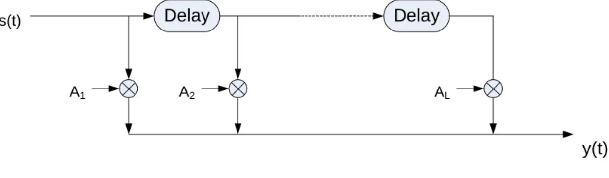
(26) ⎡ a11( l ) ⎤ ⎢ (l ) ⎥ ⎢ a21 ⎥ ⎢ ⎥ ⎢ (l ) ⎥ ⎢ aM 1 ⎥ ⎢ a (l ) ⎥ ⎢ 12(l ) ⎥ Al = ⎢ a22 ⎥ ⎢ ⎥ ⎢ ⎥ ⎢ aM( l )1 ⎥ ⎢ (l ) ⎥ ⎢ a13 ⎥ ⎢ ⎥ ⎢ (l ) ⎥ ⎣ aMN ⎦ MN ×1. ⎡ a1( l ) ⎤ ⎢ (l ) ⎥ ⎢ a2 ⎥ al = ⎢ a3( l ) ⎥ ⎢ ⎥ ⎢ ⎥ ⎢a ( l ) ⎥ ⎣ MN ⎦ MN ×1. (2.19). where al is a vector with M × N uncorrelated fading elements. The simulator structure proposed in [9] is illustrated in Figure 2.6. First the target simulation environment is decided. Next, the simulation parameters are set according to the chosen environment. From the desired parameters, the spatial correlation matrix, the power delay profile and the Doppler shift can also be chosen properly. Note that in Figure 2.6(a), s(t) and y(t) are transmitting and received signals in MIMO systems.. (a). 13.

(27) Delay. s(t). A1. Delay. A2. AL. y(t) (b) Figure 2.6 Simulator structure diagram for generating spatial correlated fading model (a) simulator flow diagram (b) signal flow diagram. 2.2.2 Studies and Simulation Results Our Matlab simulation flow is shown in Figure 2.7. First of all, a single fading channel is constructed based on Jakes’ model. After that, spatial correlation property is added to the channel simulator. At last, the channel response is produced by this MIMO channel simulator.. Figure 2.7 Simulation flow of the adopted MIMO channel simulator. 14.

(28) 0.7 Fading coefficient by Simulator Theoretical Curve ( Rayleigh Distribution ). Probability Distribution. 0.6. 0.5. 0.4. 0.3. 0.2. 0.1. 0. 0. 1. 2. 3. 4. 5. Magnitude. Figure 2.8 Magnitude distribution of four correlated fading channels. In the simulation, it shows that Jakes’ model can model the Rayleigh fading channel precisely. The distribution of amplitude fits Rayleigh distribution and the phase variation is also uniformly distributed. In Figure 2.8 and 2.9, it can be observed that the distributions of magnitude and phase are close to the theoretical curve.. 15.

(29) 90. 100 Theoretical phase distribution 60 Fading coefficient by Simulator 80. 120. 60 150. 30. 40 20. 180. 0. 210. 330. 240. 300 270. Figure 2.9 Phase distribution of four correlated fading channels (polar plot). To verify the spatial correlation property, a 4 by 4 correlation matrix (as listed in Table 2.1) is selected to be target correlation matrix as an example.. Table 2.1 Desired spatial correlation matrix of the channel simulator. Channel 1. Channel 2. Channel 3. Channel 4. Channel 1. 1. 0.3. 0.3. 0.3. Channel 2. 0.3. 1. 0.3. 0.3. Channel 3. 0.3. 0.3. 1. 0.3. Channel 4. 0.3. 0.3. 0.3. 1. 16.

(30) Table 2.2 Resulting spatial correlation matrix of the channel simulator. Channel 1. Channel 2. Channel 3. Channel 4. Channel 1. 1. 0.324. 0.2655. 0.2863. Channel 2. 0.324. 1. 0.2898. 0.2436. Channel 3. 0.2655. 0.2898. 1. 0.2831. Channel 4. 0.2863. 0.2436. 0.2831. 1. In the simulation, the resulting correlation matrix (as listed in Table 2.2) approximates to the desired matrix. This method can model the spatial correlation well. If we can adjust the number of oscillator in the Jakes’ model, the matrix can be more precise, but it will take more computation time (i.e., take more iterations for simulation).. 17.

(31) 18.

(32) Chapter 3 Standards of IEEE 802.11n (WWiSE) and IEEE 802.16a. For the rapid increase of broadband wireless communication, MIMO techniques are integrated into communication system to enhance system performance. However, the adoption of MIMO OFDM architectures may cause some difficulties in synchronization and channel equalization. For this reason, some efficient channel estimation schemes must be studied. Since a few years ago, some new communication standards have been discussed in the forums held by global engineering society, such as IEEE. One of them is MIMO 802.11n, which is a performance-enhanced version of 802.11-series standards. Another standard is 802.16a for wireless metropolitan area network (Wireless MAN). It also defines a specific optional mode with space-time block coding (STBC). In this chapter, we will make a simple introduction for both existing industrial standards with MIMO OFDM architectures.. 3.1 IEEE 802.16a standard The first version of P802.16a draft was issued on 30 November 2001. The last version of draft P802.16/D7 (draft version 7) was issued on 11 December 2002. The formal document of IEEE 802.16a (also known as WinMax) was approved as an IEEE standard on 29 January 2003 by IEEE Standard Association. The standard is developed by IEEE 802.16 Working Group and then the IEEE 802 Executive Committee. IEEE 802.16a focuses on the application of wireless metropolitan area, 19.

(33) network (Wireless MAN). This application may replace present ‘last mile’ technology between users’ terminals and Internet service providers (ISP). Wireless MAN may be a threatening competitor against wired communication technologies, such as ADSL or VDSL. We will introduce main features of 802.16a in the following subsections.. 802.16a defines three system modes: single carrier (SC), OFDM, and OFDMA. Each mode corresponds to different applications. OFDMA mode with space-time coding will be focused in this thesis. Table 3.1 shows the key baseband parameters of 802.16a-2003 standards. Some common abbreviations and expressions of 802.16a OFDMA PHY standard are listed below before introducing technical detail for conciseness.. (1)SS (subscriber station): usually known as user station or mobile stations. (2)BS (base station): equipment sets providing connectivity, management, and control of subscriber stations. (3)MAC (media access control): used to control system access and provides links of data from upper layer (data link layer) and lower layer (physical layer). (4)PHY (physical layer): handles the data transmission and may include use of multiple transmission technologies, each appropriate to a certain frequency and application. (7)TDD (time division duplexing): a single channel is used for both upstream and downstream transmission, but at different time. (8)FDD (frequency division duplexing): requires two different channel pairs, one for upstream and another for downstream data transmission. (9)STC (space-time coding): a coding skill applied on spatial and time domains. 20.

(34) Table 3.1 Main baseband features of 802.16a-2003. Band Allocation. 2-11Ghz. Throughput. 1.0-75.0Mbps. Coverage range. Most 32km,(6-9km is a typical range). Mobility. Fixed. Channel model. nLOS. Bandwidth. 1.25-20Mhz. PHY. SCa, OFDM,OFDMA. 3.1.1 802.16a OFDMA Frame and Symbol Structures The adopted duplexing methods are either FDD or TDD. The frame structures are different in these two duplexing methods. In license-exempt bands, the duplexing method is defined as TDD, which will be described in the following part. A typical OFDMA TDD time frame is shown in Figure 3.1. We can see that the DL and UL bursts are inserted into different time slots on all the subchannels. Between DL and UL bursts, narrow time gaps are inserted to protect different bursts from inter-frame interference. The time gaps are named as Tx/Rx transition gap (TTG) and Rx/Tx transition gap (RTG). The receivers at BS and SS should detect the beginnings of their corresponding bursts, and then start other following detection steps.. 21.

(35) Figure 3.1 Frame structure of 802.16a OFDMA [11]. As described in Chapter 2 and Figure 3.2, a symbol (Ts) of 802.16a is composed of useful symbol (Tb) and guard interval (GI). The purpose of GI is to reserve orthogonality of each subcarrier, as we have described in Chapter 2.. Tg Tb Ts. Figure 3.2 Time-domain structure of a 802.16a symbol. 22.

(36) In frequency domain, all the subcarriers are either data carriers, pilot carriers, or guard band carriers. The purpose of guard band carriers are to avoid interference from other radiation sources or communication systems located at nearby bands, and the pilot carriers are for channel estimation or other tracking procedures. The data carriers are grouped into several subchannels, and data streams from different SS may transmit on different subchannels. The frequency domain description is shown in Figure 3.3.. Figure 3.3 802.16a symbol frequency domain structure. 3.1.2 802.16a OFDMA Carrier Allocation In 802.16a OFDMA, the standard specifies the data tones and pilot tones in different ways for downlink and uplink. In general, an OFDMA symbol obtains a set of used subcarriers excluding DC subcarrier and guard band subcarriers. In both uplink and downlink, these used subcarriers are divided into data tones and pilot tones. However, the allocation of data and pilot tones is different in uplink and downlink. The main difference is that the pilot carriers are allocated first and then all the other data carriers are grouped into 32 subchannels in downlink, and the pilot carriers are allocated in each subchannel. But in uplink, each subchannel has its own set of pilot carriers. This allocation corresponds to the fact that BS broadcasts to all SS in the downlink transmission, and SS delivers data stream individually to BS in the uplink transmission. In this thesis, we will mainly discuss the design of channel estimation in DL. 23.

(37) In DL of 802.16a OFDMA, all of the subcarriers can be divided into pilot tones and data tones according to the different purpose in data transmission. The pilot tones can be categorized into fixed location pilots and variable location pilots. There are 32 fixed-location pilot in an OFDM symbol, and their exact positions are listed in the 14th row of Table 3.2. The allocations of DC subcarrier and guard band subcarriers are also listed in the first three rows of Table 3.2. These special tones are allocated at the same places in every OFDM symbol. However, there are many variable location pilots other than those fixed-location ones. These variable location pilots repeat with a period of four OFDM symbols. The placement of variable location pilots is decided by equation (3.1). varLocPilotk = 3L + 12 Pk ,. where L is the offset that cycles through the values 0,1,2,3, periodically.. (3.1). Pk ∈ {0,1, 2, 141}. The variable location pilots described in (3.1) are specially designed that the number of overall pilot tones are the same in every OFDM symbol even if there are variable location pilots coinciding with fixed location pilots. Additionally, there won’t be all -pilot preamble in the DL OFDM symbols. Five 802.16a OFDMA DL symbols are illustrated in Figure 3.4 to show how these pilot tones are allocated, and the periodicity of variable pilots is also shown.. 24.

(38) Figure 3.4 Carrier Allocation of DL 802.16a OFDMA [11] Table 3.2 Detailed Carrier Allocation of DL 802.16a OFDMA [11]. 25.

(39) 3.1.3 802.16a OFDMA Space-Time Coding (STC) In 802.16a standard, a simple scheme of transmitter diversity is defined as an optional mode. The special optional mode is mainly based on Alamouti’s scheme [2]. In this optional mode, we assume that the number of antennas at BS is two and the number at SS is one. A simple illustration of BS and SS is shown in Figure 3.5. The process before TX diversity encoder is quite similar to the general mode configuration. However, after the diversity encoder, the new space-time code words are modulated by two independent IFFT processors. Once the transform is completed, the OFDM symbols are converted into analog signal, and then they will be transmitted on different antennas of BS. For this special transmission mode, BS will require extra hardware in its design. This modification is also shown in the upper part of Figure 3.5.. Table 3.3 Encoding pattern of 802.16a STC mode. Antenna 0 time t time t+T. Antenna 1. S0. S1. -S1*. S0*. Detailed encoding flow of Tx diversity encoder is described in Figure 3.6. The encoding procedures are applied to each subcarrier and both on space and time domains. Table 3.3 gives a clear description on this procedure.. 26.

(40) Figure 3.5 Tx/Rx architecture of 802.16a with STC [11]. Figure 3.6 Transmitter symbol arrangement of 802.16a STC [11]. 3.2 IEEE 802.11n WWiSE Proposal According to WWiSE 802.11n proposal [12], the frame structure of this system is quite similiar to 802.11a system. The proposal keeps major features of 802.11a to sustain backward-compatibility to the legacy system. The frame structure of 802.11a will be explored, and then extended to WWiSE’s proposed system.. 27.

(41) 3.2.1 Physical Layer Parameters of WWiSE The system operates at 5 GHz license-free band, which has an advantage of large bandwidth for license-exempt usages. The system has a sampling rate of 20 MHz and FFT length of 64 points. A typical OFDM block duration consists of 80 samples. 64 samples of them are modulated data and 16 samples for guard interval, and their purposes have been introduced in 2.1.2 already. Among the total 64 subcarriers of an OFDM symbol, 12 tones on both sides of channel band are guard band to avoid interference to other nearby system. Besides 4 pilot tones, 48 subcarriers are used for data transmission. The main features of WWiSE physical layer are listed in Table 3.4.. Table 3.4 Main features of WWiSE baseband Mandatory Mode. Sampling rate. 20MHz. Number of FFT points. 64. Number of data subcarriers. 48. Number of pilot subcarriers. 4. Subcarrier spacing. 0.3125 MHz (=20MHz/64). OFDM symbol period. 4µs (80 samples). Cyclic prefix period. 0.8µs (16 samples). FFT symbol period. 6.2µs (64 samples). Modulation scheme. BPSK,QPSK,16QAM,64QAM. Short training sequence duration. 8µs. Long training sequence duration. 8µs. Long training symbol GI duration. 1.6µs. 28.

(42) 3.2.2 Frame Structure of WWiSE Mandatory Mode Figure 3.7 shows the basic structure of an 802.11a frame. A frame consists of three parts, which are Preamble, SIGNAL, and DATA, respectively. Preamble part is inserted into the frame to assist synchronization and channel estimation. SIGAL part contains the length, modulation type, ECC coding rate, and other information of following DATA part. The modulation of SIGNAL is fixed to BPSK, and the coding rate of convolution code is 1/2. DATA part is the main element of a whole frame and carries data from transmitter. This thesis will focus on channel estimation skills. Our studies will be concentrated on design of Preamble part.. Figure 3.7 Frame structure of WWiSE 802.11n proposal [13]. In Figure 3.8, a clear illustration of 802.11a frame is shown. This figure shows two types of training field, the short training field (STF) and long training field (LTF). In the advice of IEEE standard [14], there are ten STFs for auto gain control (AGC), coarse frequency offset estimation, and timing synchronization. After these STFs, there are two LTFs for channel estimation. In Chapter 4, we will focus on the arrangement of LTFs to complete our channel estimation.. 29.

(43) Figure 3.8 Detailed frame structure of 802.11n system [13]. In [12], WWiSE proposed a prototype system for 802.11n MIMO OFDM system based on 802.11a standard as we mentioned in this subsection. For example, if there are two transmitting antennas, training sequence of the first antenna is similar to 802.11a, and training sequence of the second antenna will be cyclic-shift version of the first antenna. This special structure is shown in Figure 3.9. Note that guard interval GI21 in this figure is cyclic-shift version (1600ns) of GI2. We can extend this case to four-antenna scenario as we show in Figure 3.10. The shift length is described in each field of this figure. In following discussion, the case of two antennas will be focused for simplicity consideration.. Figure 3.9 Frame structure of WWiSE system with two transmission antennas [12]. 30.

(44) Figure 3.10 Frame structure of system WWiSE with four transmission antennas [12]. 3.2.3 The Code Structure of Space-time Block Code From Table 3.3, the transmission model of space-time block code can be described in following equations. Assume the channel responses h0 and h1 are static in a STBC symbol (two consecutive OFDM symbols).. h0 (t ) = h0 (t + T ) = h0 = α 0 e jθ 0 h1 (t ) = h1 (t + T ) = h1 = α 1e jθ1. (3.2). And the received signal r0 and r1 are. r0 = r (t ) = h0 S o + h1 S1 + v0 r1 = r (t + T ) = −h0 S1 + h1 S 0* + v1 *. Finally, we define the estimated signal Sˆ0 and Sˆ1 as. 31. (3.3).

(45) h *r + h r * Sˆ0 = 0 20 1 12 h0 + h1 Sˆ1 =. (3.4). h1*r0 − h0 r1* 2. h0 + h1. 2. Substituting (3.2) to (3.4), we get h *v + h v * Sˆ0 = S0 + 0 20 1 21 (α 0 + α1 ). (3.5). − h v * + h1*v0 Sˆ1 = S1 + 0 21 (α 0 + α12 ). When the number of data streams is three and four, we use the following space-time block codes, H3 and H4, to encode the data. The decoders for H3 and H4 are derived in the Appendix of [14].. ⎛ ⎜ S1 ⎜ ⎜ * ⎜ − S2 H3 = ⎜ * ⎜ S3 ⎜ 2 ⎜ * ⎜ S3 ⎜ ⎝ 2 ⎛ ⎜ S1 ⎜ ⎜ * ⎜ − S2 H4 = ⎜ * ⎜ S3 ⎜ 2 ⎜ * ⎜ S3 ⎜ ⎝ 2. −. S3 −. 2 * * S S2 − S2 − + 1 1 2 * * S 2 + S 2 + S1 − S 1 2. (− S. *. 2 * S3. (. 2. ). *. 2 * S3 2. ). ⎞ ⎟ ⎟ ⎟ ⎟ ⎟ ⎟ ⎟ ⎟ ⎟ ⎟ ⎠. (3.6). S3. 2 S3. *. S3. S1. 2 S3. *. S3. S2 S1. S3. S2. 2 * * − S1 − S 1 + S 2 − S 2 2 * * S 2 + S 2 + S 1 − S1 2. (. (. ). 32. −. 2 S3. 2 * * S S 1 − S1 − + 2 2 2 * * S1 + S 1 + S 2 − S 2 − 2. ) (− S. ). (. ). ⎞ ⎟ ⎟ ⎟ ⎟ ⎟ ⎟ ⎟ ⎟ ⎟ ⎟ ⎠. (3.7).

(46) Chapter 4 Channel Estimations for MIMO OFDM Systems. 4.1 Preamble Design for MIMO OFDM Systems In [15], several types of pilot arrangements are proposed for MIMO OFDM systems. In this thesis, three of them will be discussed. In this section, these pilot arrangement methods will be introduced briefly. The pilot arrangements concerned are all-pilot preamble, space-time coded preamble, and scattered preamble, respectively. The same spatial arrangement may combine different time-frequency preamble formats, such as block type (802.11n) and comb type (802.16a with STC). A simple category of pilot arrangement is shown in Figure 4.1. After a general study, channel estimation in both 802.11n and 802.16a systems will be discussed.. 33.

(47) Figure 4.1 Classification of pilot arrangement in MIMO OFDM. 4.1.1 Scattered Preamble This preamble format is proposed in [15]. The scattered pilot preambles organize subcarriers in a single all-pilot-preamble symbol into several groups for different antennas. The transmission signal on each antenna can be expressed in the form of (4.1) and (4.2). The illustration of scattered preamble and data symbols is shown in Figure 4.2.. For pilot symbol assisted modulation (PSAM) OFDM symbol X1 = (P 0 d d P 0 d d. ). X 2 = (0 P d d 0 P d d. ). (4.1). where P is pilot tone and d is data tone. For block type OFDM preambles (802.11n-like) X1 = ( P 0 P 0 P 0 P 0. ). X 2 = (0 P 0 P 0 P 0 P. ). 34. (4.2).

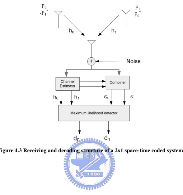
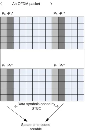
(48) Pilots for first antenna Pilots for second antenna An OFDM packet. Data symbols coded by STBC. All-pilot preamble. Figure 4.2 Frame structure of a 2x1 MIMO OFDM system with scattered pilot. 4.1.2 Space-time Coded Preamble According to [2], space-time block code (STBC) can be applied to MIMO system so that the diversity of multiple antenna systems can be utilized. If the transmitted symbols are known, one can obtain the channel response from space-time coded OFDM symbols. The transmission scheme of this space-time coded preamble is depicted in Figure 4.3, and it can be seen how channel estimator (for preambles) and combiner (for data symbols) work. Table 4.1 lists transmission sequence of the space-time symbols between two antennas, and Figure 4.4 shows total arrangement of a whole packet in this kind of pilot arrangement.. 35.

(49) Figure 4.3 Receiving and decoding structure of a 2x1 space-time coded system. Table 4.1 Training symbol arrangement of space-time coded preamble. Antenna 0 time t time t+T. Antenna 1. P0. P1. -P1*. P0*. 36.

(50) An OFDM packet P0 -P1*. P0 -P1*. P1 P0*. P1 P0*. Data symbols coded by STBC. Space-time coded preable. Figure 4.4 Frame structure a 2x1 MIMO OFDM system with space time coded pilot. 4.1.3 All-pilot Preambles In a SISO OFDM system with packet transmission, the all-pilot preambles are often used. As introduced in Section 3.2.2, 802.11a system adopts this frame structure to perform channel estimation with its LTF preambles. If 802.11n system is needed to backward-compatible to 802.11a, the 802.11n system must reserve the feature of all-pilot preambles. As explained in section 3.2.2, WWiSE uses cyclic-shift version of original LTF for antennas other than the first one. However, this structure may experience severely co-channel (CCI) effect because pilots from different antennas occupy the same tones at the same time. For scattered preambles and space-time coded preambles mentioned previously, this problem can be avoided by tone-interleaving skills and space time block coding. The issue of CCI cancellation will be discussed later in this chapter. 37.

(51) 4.2 Channel Estimation Techniques for MIMO OFDM System In [16], the authors mainly introduce the methods to detect channel response on pilot tones based on LS and MMSE methods for SISO OFDM systems. For MIMO OFDM systems, the channel estimation problems may be more complicated. Due to the special structure of space-time coding and co-channel interference, some additional processing must be integrated into the MIMO OFDM system to solve these problems. In this section, we will study channel estimation methods for MIMO OFDM systems.. 4.2.1 Channel Estimation for Scattered Preambles Scattered preamble described in (4.2) is explored further here. To explain the estimation process, an example is given. The number of transmitter antennas is two, and the total amount of subcarriers in an OFDM symbol is 64. In this case, the frequency domain expression of two OFDM preambles P1 and P2 can be described by (4.3).. P1 = ( P01 0 P21 0 P41 0 P2 = (0 P12. 0 P32. 0 P52. P621. 0). 0 P632 ) th. m k. P is the pilot symbol at tone k from the m antenna. 38. (4.3).

(52) In preamble symbol which belongs to a transmission packet, the channel effect and additive white noise can be modeled as. 2. R (k ) = ∑ H m (k ) Pk + w( k ) m. m =1. R (k ) is the received symbol,. (4.4). and H m (k ) is the response at the k. th. th. tone from the m antenna. Therefore, the received symbol vector R is R = [ H1 (0) P01. H 2 (1) P12. H1 (2) P21. H 2 (3) P32. For H1 estimation, the tones R(0) R(2). H1 (62) P621. H 2 (63) P632 ] (4.5). R(62) may be used for LS. estimation. The general form of estimation is like (4.6). The result can be also applied to channel response for the second antenna, and the extension to more than two antennas is straightforward. R(k ) Hˆ 1 (k ) = 1 , Pk. (4.6). k = 2t , 0 ≤ t ≤ 31 However, only half the tones are obtained when the estimation in (4.6) is applied. The response on the tones occupied by training symbol from another antenna must be derived with interpolation techniques. In following discussion, some popular interpolation techniques are considered.. 4.2.1.1 Piecewise Linear Interpolation Linear interpolation is quite simple and intuitive among all interpolation skills. The interpolation skills are based on linearity assumption of unknown subcarrier responses between known two known subcarrier intervals. If known subcarrier data is inserted for each M subcarrier, the segment length is M, and then subcarrier response interpolation in the mth segment can be obtained by. 39.

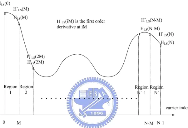
(53) M -l ˆ l Hˆ (mM + l ) = H (mM ) + Hˆ ((m + 1) M ) , 0 < l < M M M. (4.7). 4.2.1.2 SPLINE Interpolation. Figure 4.5 Illustration of channel segmentation and the required known parameters for cubic spline interpolation. For generalization, specific-order spline functions can be derived such as the widely used cubic spline for channel interpolation. It is based on the third-order 3. 2. curve-fitting polynomial Yi = Axi + Bxi + Cxi + D . Sufficient equations are required to solve this problem because there are total 4N’ unknown variables. All the divisional polynomial coefficients are solved based on continuous assumption at the segment boundary, with the first and second derivative continuity of the pilot channel values on segment boundaries. Therefore, (2N’)+(N’-1)+(N’-1) equations can be set. 40.

(54) up from the constraints, with two more from the assumption of zero first order derivative value of the very first and last carrier channel value.. 4.2.1.3 Transform-Domain Interpolation DFT-based channel estimators have been proposed in [17,18]. These estimators are based on the techniques performed in transform domain to accomplish the estimation. Fast DFT algorithms can be utilized to reduce the transform complexity. In the following, we will describe this method in detail. The DFT-based channel estimator has a principal restriction on placement of pilot subcarriers. That is, pilot subcarriers must be equi-spaced along frequency direction. A typical pilot pattern is shown in Figure 4.6. As the figure describes, DFT estimator can be applied only when D f is a constant. In such case, pilot tones can be viewed as a downsampled version. of frequency response on all tones. pilot. data. Df. Df y c n e u q e r F Time. Figure 4.6 Regular pilot placement. When scattered pilots are used in MIMO OFDM, interpolations are needed to obtain channel response of interleaving tones for different antennas. In this case, transform domain methods are good choices because of the equi-spaced pilot tones in preambles. 41.

(55) We can find different channels between different antenna pairs with interpolation skills.. In this subsection, we will discuss non-sample spaced channel effect in general wireless channels. As mentioned in Chapter 2, radio channel impulse responses can be modeled as several delay paths with random distributed gain (usually Rayleigh distribution). However, delay intervals are always assumed to be sample spaced. In real transmission environment, this assumption is not true for most cases. In the following parts of this subsection, this effect will be explored while transform-domain interpolation methods are used in MIMO OFDM channel estimation.. According to [19], the continuous channel impulse response can be expressed in (4.8), where v is the total number of channel delay taps, and ε l is delay time for each tap. In (4.9), the frequency domain response is obtained by DFT, where τ l is the delay interval normalized to sampling period Tc . And Tc equals to T/N. ν −1. h(t ) = ∑ α lδ (t − ε l ). (4.8). l =0. ν −1. H discrete (k ) = ∑ α l e. − j 2π k. εl NTc. l =0. k = 0,1, 2. ν −1. = ∑αl e. −j. 2π kτ l N. l =0. , N −1. (4.9). Tc ≡ sampling period To obtain the equivalent discrete-time impulse response, IDFT is performed on. H discrete (k ) .. 42.

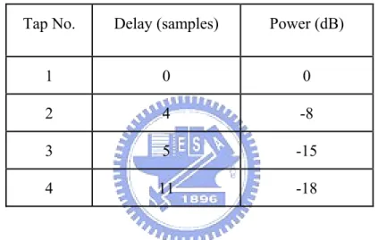
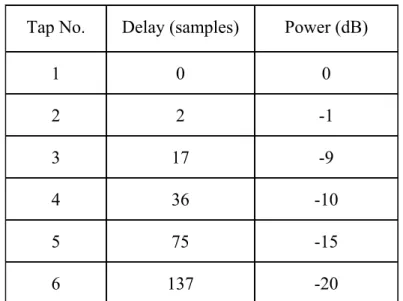
(56) hdiscrete (n) = IDFT {H discrete (k )} 1 = N. ν −1. ∑ α (iT )e l =0. l. −j. π ( n + ( N −1)τ l ). s. N. sin(πτ l ) , n = 0,1, 2, sin(π (τ l − n) / N ). (4.10) , N −1. If the delay intervals are all sample-spaced, i.e. {τ l } are all integers, hdiscrete (n) can be simplified to ν −1. hdiscrete (n) = ∑ α l (iTs )δ (n − τ l ),. n = 0,1, 2,. , N −1. l =0. Table 4.2 Channel parameters for indoor wireless channel (Model 1). Tap No.. Delay (ns). Delay. Power (dB). (samples). Amplitude Distribution. 1. 0. 0. 0. Rayleigh. 2. 36. 0.72. -5. Rayleigh. 3. 84. 1.68. -13. Rayleigh. 4. 127. 2.54. -19. Rayleigh. Table 4.3 Channel parameters for indoor wireless channel (Model 2). Tap No.. Delay (ns). Delay. Power (dB). (samples). Amplitude Distribution. 1. 0. 0. 0. Rayleigh. 2. 176. 3.52. -8. Rayleigh. 3. 274. 5.48. -15. Rayleigh. 4. 560. 11.2. -18. Rayleigh. 43. (4.11).

(57) According to (4.8)-(4.10), the continuous channel response and the discrete channel response can be both illustrated in Figure 4.7 and Figure 4.8. The channel model is cited from [20]. Model 1 is in the environment of typical office, and Model 2 is in an airport hall. In Figure 4.7 and Figure 4.8, one can see that the delay spread of Model 1 is smaller than Model 2, which means that the delay taps are more concentrated in Model 1 than in Model 2. By observing the impulse response plot in Figure 4.7, we can see the aliasing effect in ‘high time’ part due to non-sample spaced channel. However, this effect seems not very obviously in Model 2. To explain this effect, we may examine (4.8)-(4.10) to find the answer. If we check sinusoid ratio part in (4.10), it would become (4.12). w(n) =. 1 sin(πτ l ) × N sin(π (τ l − n) / N ). (4.12). Equation (4.12) can be viewed as the gain of interference produced by other taps in continuous impulse response. It is plotted in Figure 4.9. Here, τ l = 4.48 and N=64 are chosen as an example. It can be seen that Model 2 has larger attenuations on the multipath taps other than the main path. Additionally, the multipath taps are located at loose positions, so that the introduced aliasing effect is smaller than in Model 1. Therefore the aliasing effect is not so significant in Model 2.. 44.

(58) 1 Discrete Channel Impulse Response 0.9. Original Continuous Channel Impulse Response. 0.8 0.7. Maginitude. 0.6 0.5 0.4 0.3 0.2 0.1 0. 0. 5. 10. 15. 20. 25. 30 35 40 Tap Delay (samples). 45. 50. 55. 60. Figure 4.7 Continuous and discrete impulse responses of indoor model 1. 1.4 Discrete Channel Impulse Response Original Continuous Channel Impulse Response. 1.2. Maginitude. 1. 0.8. 0.6. 0.4. 0.2. 0. 0. 5. 10. 15. 20. 25 30 35 40 45 Tap Delay (samples). 50. 55. 60. Figure 4.8 Continuous and discrete impulse responses of indoor model 2. 45.

(59) 0.7. 0.6. Maginitude. 0.5. 0.4. 0.3. 0.2. 0.1. 0. 0. 10. 20. 30 40 n (samples). 50. 60. 70. Figure4.9 Magnitude plot of tap weight of non-sample spaced channel. Unfortunately, DFT-based channel [17] estimator is sensitive to non-sample spaced channel effect. Therefore the DCT-based estimator [19] is applied to this kind of MIMO OFDM system to improve the performance of transform domain channel estimator. In remaining part of this subsection, we will explain how non-sample spaced effect impacts the performance of typical DFT-based estimator. After that, we will show how DCT-based channel estimator compensates this drawback.. The DFT-based estimator starts with Least Square estimation of channel frequency response at pilot subcarriers. The LS estimation is described by (4.13). We assume the maximum delay spread is τ maxTc and ∆ is the minimum integer that is larger than τ max . Then we shift the channel impulse response by − ∆ / 2 so that the. 46.

(60) power of channel impulse response is centered around n = 0. The shift process can be carried out by phase rotation in the frequency domain, as shown by equation (4.14). Y (k ) N (k ) = H p (k ) + p = H p (k ) + N p (k ) Hˆ p (k ) = p P(k ) P(k ) where Hˆ (k ) isthe estimated response at k th subcarrier, p. (4.13). Yp (k ) is the received signal, P(k ) is the pilot, and N p (k ) is noise ∆k. jπ Hˆ ′p (k ) = Hˆ p (k ) × e M. (4.14). where M is the number of pilot tones Next, M-point IDFT of Hˆ ′p (k ) is performed. {. }. 1 hˆ p (n) = IDFTk Hˆ ′p (k ) = M. M −1. ∑ Hˆ ′p (k )e. −j. 2πnk M. n = 0,1,2,. , M −1. (4.15). k =0. By the concept of interpolation, the estimated channel impulse response is obtained by zero padding. To reduce the aliasing effect, zeros must be padded to the region with less power. Sine we have centered the power around n = 0, zeros are padded in. {. }. the middle of hˆ p ( n). M −1. n=0. .. ⎧hˆp (n) ⎪ hˆ(n) = ⎨ 0 ⎪ hˆ ( M + n − N ) ⎩ p. 0 ≤ n ≤ M / 2 −1 otherwise N - M / 2 ≤ n ≤ N −1. (4.16). After that we perform N-point DFT on hˆ(n) , which results in interpolation in frequency domain, as shown below. N −1. −j H ′(k ) = ∑ hˆ(n)e. 2πnk N. k = 0,1,2,. , N −1. (4.17). n=0. Finally, the estimated channel frequency response Hˆ ( k ) is obtained by removing phase rotation effect from H ′(k ) .That is (4.18). Hˆ (k ) = H ′(k ) × e. − jπ. ∆k N. k = 0,1,2, 47. , N −1. (4.18).

(61) The whole estimation process of DFT-based estimator is shown in Figure 4.10.. Hˆ p (k ). Y p (k ). Hˆ ′p (k ). hˆ p (n) Hˆ (k ). H ′(k ). hˆ(n). Figure 4.10 DFT-based channel estimator. Basic idea of the DCT-based channel estimator [19] is to make the input data symmetric so that the high frequency component is reduced, and then apply DFT-based interpolation algorithms. As a result, IDCT or DCT based channel estimation will be obtained. Although mirror-duplicating can be done in time domain, it can also be done by defining the extended pilot channel frequency response as [19] ⎧ Hˆ (k ) ⎪⎪ p ˆ H 2 M (k ) = ⎨ 0 jπ ( 2 M − k ) − ⎪ˆ M ⎪⎩ H p (2M − k )e. 0 ≤ k ≤ M −1 k=M. (4.19). M + 1 ≤ k ≤ 2M − 1. This design is compatible with the conventional inverse discrete cosine transform. For both two approaches, high frequency components are less significant than DFT-based approach, because the processed data are symmetric. Therefore, interpolation by using Hˆ 2M ( k ) would be better than the original DFT-based estimation.. With Hˆ 2 M (k ) , we can perform its DFT-based interpolation to get the estimated channel frequency response. To achieve IDCT/DCT-based algorithm, each step of DFT-based estimator will be translated to DCT-related operation. First, we perform IDFT on the extended Hˆ 2 M ( k ) to get the time-domain signal 48.

(62) 1 hˆ2 M (n) = 2M =. 2 M −1. ∑ k =0. Hˆ 2 M (k )e. j 2π nk 2M. 1 ˆ 1 H 2 M (0) + 2M 2M. j 2π nk j 2π nk − ⎡ˆ ⎤ 2M 2M ˆ H k e + H M − k e ( ) (2 ) ∑ ⎢ 2M ⎥ 2M k =1 ⎣ ⎦. M −1. 1 ˆ 1 M −1 − 2jπMk ˆ (2n + 1)π k 2e ) H p (0) + H p (k ) cos( ∑ 2M 2M k =1 2M 1 M −1 (2n + 1)π k = ) w(k )Hˆ ′p (k ) cos( ∑ 2M 2M k =0 1 ˆ = n = 0,1, 2, , 2M − 1 h( n ) 2M ⎧ 1 ˆ H p (k ) k =0 ⎪⎪ where Hˆ ′p (k ) = ⎨ 2 and hˆ2 M (n) = hˆ2 M (2 M − n − 1) jπ k ⎪ − 2M ˆ H p (k ) 1 ≤ k ≤ M − 1 ⎪⎩ e ⎧ 1 ⎪ M k=0 ⎪ and w(k)= ⎨ ⎪ 2 k≠0 ⎪⎩ M =. (4.20). This shows that the time-domain signal hˆ2 M ( n) can be obtained by performing IDCT on Hˆ ′p (k ) followed by a constant multiplication. Next, continuing the interpolation by zero-padding hˆ2 M ( n) , we can get the corresponding time-domain signal to the target upsampled channel response, which is what we want to solve in the end. ⎧ hˆ2 M (n) ⎪ hˆ2 N (n) = ⎨ 0 ⎪hˆ (n − 2 N + 2 M ) ⎩ 2M. 0 ≤ n ≤ M −1 otherwise. (4.21). 2N − M ≤ n ≤ 2N − 1. Finally, the estimated channel frequency response is obtained by performing DFT on hˆ2 N (n) .. 49.

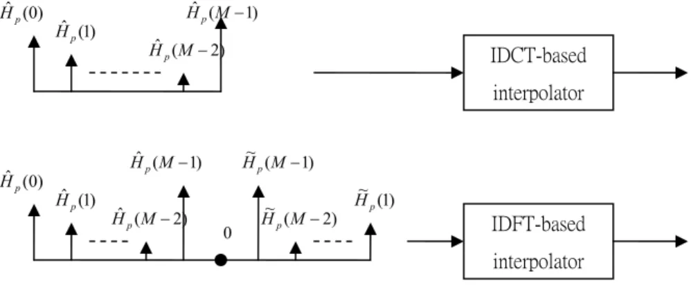
(63) Hˆ 2 N (k ) = =. 2 N −1. − ∑ hˆ2 N (n)e. n =0 M −1. − ∑ hˆ2 M (n)e. j 2πnk 2N j 2πnk 2N. 2 N −1. − ∑ hˆ2 M (n − 2 N + 2M )e. +. n =0 M −1. j 2πnk 2N. n=2 N −M. j 2π ( 2 N −1− n ) k j 2πnk − − ⎡ˆ ⎤ 2N 2N ˆ = ∑ ⎢h2 M (n)e + h2 M (2 M − n − 1)e ⎥ n=0 ⎣ ⎦ j 2πnk j 2π ( n +1) k M −1 ⎡ − ⎤ 1 2N = + hˆ(n)e 2 N ⎥ ⎢hˆ(n)e ∑ 2 M n =0 ⎣ ⎦ jπk M −1 (2n + 1)πk 1 = ) e 2 N ∑ 2hˆ(n) cos( 2N 2M n =0 M −1 (2n + 1)πk = wk′ wk ∑ hˆ(n) cos( ) 2N n =0. where wk′ =. 1 2. k = 0 , w′k = e. jπk 2N. k = 1,2,. (4.22). , N −1. This equation is equivalent to a DCT operation combined with one constant multiplication. It is obvious that in the interpolation process, hˆ(n) can be obtained by IDCT and Hˆ 2 N (k ) is the DCT transform of hˆ(n) followed by one multiplication. Therefore, the whole IDFT-based interpolation can be replaced by DCT-based operations. This IDCT/DCT-based channel estimator [19] is shown in Figure 4.11. We also show the equivalent channel estimations by IDCT-based interpolator and IDFT-based interpolator in Figure 4.12, where πk. −j ~ H p (k ) = Hˆ p (k )e M. Y p (k ). k = 1,2,. Hˆ p (k ). , M −1. (4.23). Hˆ ′p (k ). hˆ(n) Hˆ (k ). H ′(k ). Figure 4.11 IDCT/DCT-based channel estimator. 50.