基因演算之模糊ID3方法和其決策樹的修剪研究

國 立 交 通 大 學

電 機 與 控 制 工 程 研 究 所

碩 士 論 文

基因演算之模糊 ID3 方法和其決策樹的修剪研究

Genetic Algorithm Based Fuzzy ID3 Method and Its

Pruning Study

研 究 生 ： 張 昭 銘

指 導 教 授： 張 志 永

基因演算之模糊 ID3 方法和其決策樹的修剪研究

Genetic Algorithm Based Fuzzy ID3 Method and Its

Pruning Study

學 生 : 張昭銘 Student : Chao-Ming Chang

指導教授 : 張志永 Advisor : Jyh-Yeong Chang

國立交通大學

電機與控制工程學系

碩士論文

A Thesis

Submitted to Department of Electrical and Control Engineering

College of Electrical Engineering and Computer Science

National Chiao Tung University

in Partial Fulfillment of the Requirements

for the Degree of Master in

Electrical and Control Engineering

July 2006

Hsinchu, Taiwan, Republic of China

基因演算之模糊 ID3 方法和其決策樹的修剪研究

學生：張昭銘

指導教授：張志永博士

國立交通大學電機與控制工程研究所

摘要

ID3 演算法是一種對於符號屬性資料的決策樹歸納且普遍有效的方法。然 而，進一步能結合人類思考與感覺的知識法則有著不精確和不確定性，為了獲取 不精確和不確定的知識，因此 ID3 決策樹方法乃推廣至模糊集語試之模糊 ID3 決策樹，它和 ID3 演算法的特徵有高度可推廣至模糊集之語試變數，並且自然擴 展到應用在包含連續數值屬性的資料集。但是模糊 ID3 演算法只能處理連續數值 資料，並且通常被批評為不夠高的辨識準確性。在本篇論文中，我們提出一個產 生模糊決策樹的新方法，它可以接受非連續數值、連續數值或混雜型的資料並使 用基因演算法調整決策樹法則相關的模糊集合。此外，我們提出三種決策樹刪減 的方法並且加以比較，進而選擇較好的決策樹刪減方法以得到更好的正確率或是 更精簡的規則庫。我們利用一些著名的資料集來測試我們所提出的方法，並且選 用最好的決策樹刪減方法，以五摺交叉評比方式的結果跟 C5.0 方法比較，在實 驗數據顯示，我們的方法有較好的結果。

Genetic Algorithm Based Fuzzy ID3 Method and Its

Pruning Study

STUDENT: CHAO-MING CHANG ADVISOR: Dr. JYH-YEONG CHANG

Institute of Electrical and Control Engineering National Chiao-Tung University

ABSTRACT

ID3 algorithm is a popular and efficient method for decision tree induction from symbolic data. However, most knowledge associated with human’s thinking and perception has some imprecision and uncertainty. For the purpose of handling imprecise and uncertain knowledge; hence, ID3 has been expanded to developed a kind of decision tree is fuzzy ID3 algorithm, which is similar to ID3 algorithm and is extended to apply a data set containing continuous attribute values. But fuzzy ID3 algorithm can only deal with continuous data and it is often criticized to result in poor learning accuracy.

In this thesis, we propose a genetic algorithm based fuzzy ID3 method to construct fuzzy classification system, which can accept continuous, discrete, or mixed-mode data sets. Furthermore, we formulate and compare three pruning methods, then choose better pruning method of decision tree to obtain better accuracy or a more efficient rule base. We have tested our method on some famous data sets, and the results of a five-fold cross validation are compared to those by C5.0. The experiments show that our method works better in practice.

ACKNOWLEDGEMENTS

I would like to express my sincere appreciation to my advisor, Dr. Jyh-Yeong Chang. Without his patient guidance and inspiration during the two years, it is impossible for me to complete the thesis. In addition, I am thankful to all my Lab members for their discussion and suggestion.

Finally, I would like to express my deepest gratitude to my family and friend, particular my parent. Without their strong support and encourage, I could not go through the two years.

Content

摘要………i

ABSTRACT………...………...ii

ACKNOWLEDGEMENTS………..………..iii

Chapter 1. Introduction………...1

1.1. Research Background………..1 1.2. Motivation………...5 1.3. Thesis Outline………..6

Chapter 2. Genetic Algorithm Based Fuzzy ID3 Method……….7

2.1. Description of the Attributes Learning………7

2.2. Feature Ranking………..8

2.3. Tree Construction………..…………14

2.4. Inference of Fuzzy Decision Tree……….………17

2.5 Genetic Algorithm for Fuzzy ID3………….……….20

Chapter 3. Pruning Methods for Fuzzy ID3………26

3.1. Introduction of Pruning method………26

3.2. Descript of Our Pruning Methods…………...………26

Chapter 4. Simulation and Experiment………35

4.2. Simulation and Comparison...………...………39

Chapter 5. Conclusion………50

List of Figures

Fig. 1.1. Machine learning process...……….….………3

Fig. 2.1. The first layer of fuzzy decision tree……….…………....16

Fig. 2.2. The full fuzzy decision tree of this example…….…….……….17

Fig. 2.3. Reasoning of the example by fuzzy decision tree..……....…….…………19

Fig. 2.4. Flowchart of genetic algorithm………..………22

Fig. 2.5. Reproduction………..……….23

Fig. 2.6. Crossover.………...……….………24

Fig. 2.7. Mutation………..………24

Fig. 2.8(a). The membership functions of “temperature.”………25

Fig. 2.8(b). The membership functions of “humidity.”.………25

Fig. 3.1(a). The credit plot on each rule: result of the first pruning method.………30

Fig. 3.1(b). The credit plot on each rule: result of the second pruning method……31

Fig. 3.1(c). The credit plot on each rule: result of the third pruning method………31

Fig. 3.2(a). Fuzzy decision tree after first pruning………32

Fig. 3.2(b). Fuzzy decision tree after second pruning...………32

Fig. 3.2(c). Fuzzy decision tree after third pruning...………33

Fig. 3.3. Flowchart of genetic algorithm based fuzzy ID3 method...………34

List of Tables

Table I. Examples of training set..………11 Table II. Examples with fuzzy representation of training set.………11 Table III. Summary of the Database Employed………....38 Table IV. Performance of the data sets before and after by the first pruning....39 Table V. Performance of the data sets before and after by the second pruning…40 Table VI. Performance of the data sets before and after by the third pruning…40 Table VII. Comparison of the accuracy with different pruning methods…………42 Table VIII. Comparison of the number of rules with different pruning methods…42 Table IX. Comparison of the testing accuracy with two better pruning methods…44 Table X. Comparison of the number of rules with two better pruning methods…45 Table XI. Accuracy comparison of our method andC5.0………..47 Table XII. Rule number comparison of our method andC5.0………48 Table XIII. Training time and executive time with our method………...………49

Chapter 1. Introduction

1.1. Research Background

Learning is very important for human being. An infant learn how to eat, how to speak and how to walk. Without learning, people are incapable to profit from their experience or to adapt to changing conditions. Learning is an essential component of any intelligent system, whether human, animal, or machine. There are two significant kinds of learning, one is acquisition of new knowledge and the other is getting new skills. With learning, system can get experience or get some knowledge form processing.

In modern life, we observe exponential growth of the amount of data and information available on the Internet and in database systems. But the data is always disorganized and difficult to understand. Researchers often use machine learning (ML) algorithm to automate the processing and extraction of knowledge from data. Inductive ML algorithms are used to generate classification rules from class-labeled examples that are described by a set of numerical (e.g., 1, 2, 4), symbolic (e.g., black, white), or continuous attributes. With analysis of the data, we can get the information or the regulations from it.

Machine learning [1] is programming computers to optimize a performance criterion using example data or past experience. We have a model defined up to some parameters, and learning is the execution of a computer program to optimize the

parameters of the model using the training data or past experience. The model may be predictive to make predictions in the future, or descriptive to gain knowledge form data, or both.

Machine learning uses the theory of statistics in building mathematical models, because the core task is making inference from a sample. The role of computer science is twofold: First, in training, we need efficient algorithms to solve the optimization problem, as well as to store and process the massive amount of data we generally have. Second, once a model is learned, its representation and algorithmic solution for inference needs to be efficient as well. In certain applications, the efficiency of the learning or inference algorithm, namely, its space and time complexity may be as important as its predictive accuracy.

The meaning of machine learning is to develop techniques to allow computers to “learn.” Briefly, machine learning is a method for analyzing of data sets by computer programs, it is better than the intuition of engineers. The system often generate knowledge form the data set, and it is often shown in the form of decision trees [2], which are the most popular choices for learning and reasoning from feature-based examples.

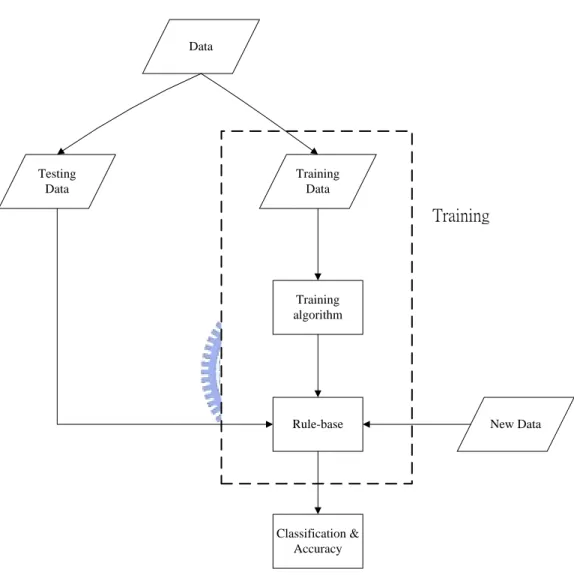
Machine learning has two stages, which finds the common properties between the set of examples in the database and classifies them into different classes, according to the model as shown in Fig. 1.1. In the first stage, we analyze the data set by the algorithm. We will get knowledge in the process which is in the form of decision rules or mathematical formulae. In the second stage, we use testing data to estimate the accuracy of the decision rules which generated previously. If the testing

accuracy is considered acceptable, the decision rules or mathematical formulae can be built as rule-base. We can use it to classify the testing data or new data examples which the categories are not known.

Data Testing Data Training Data Training algorithm Rule-base Classification & Accuracy New Data Training

Fig. 1.1. Machine learning process.

Machine learning algorithms can be categorized in several ways. In general, they are divided into supervised and unsupervised algorithms [3]. The supervised learning algorithm is told to which class each training example belongs. In case where there is no a priori knowledge of classes, supervised learning can be still applied if the data has a natural cluster structure. Then a clustering algorithm [3] has to be run first to reveal these natural groupings. In unsupervised learning, the system learns the classes

on its own. This type of learning does the classification by searching trough common properties existing among the data.

There are many ways to acquire knowledge automatically. Decision tree induction [2] has been widely used in extracting knowledge from feature-based examples for classification. A decision tree based classification method is a supervised learning method that constructs decision trees from a set of examples. The quality of a tree depends on both the classification accuracy and the size of the tree. One of the most significant developments in this domain is the ID3 algorithm, which is a popular and efficient method of making a decision tree for classification from symbolic data without much computation.

ID3 stands for “Iterative Dichotomizer (version) 3,” and is a decision tree induction algorithm, developed by Quinlan [4], and later versions including C4.5 [5] and C5.0 [6]. In the ID3 approach, we make use of the labeled examples and determine how features might be examined in sequence until all the labeled examples have been classified correctly. However, ID3 algorithm does not directly deal with continuous data. If the attributes of the training set has continuous values, the algorithms must be integrated with a discretization algorithm like CART [7] and C4.5, which transforms them into several intervals, but these decision trees are not easy to understand because we cannot know how a range of attribute is divided into intervals, and moreover most knowledge associated with human’s thinking and perception has imprecision and uncertainty. In addition, the fuzzy version of ID3 based on minimum fuzzy entropy was proposed. Investigations to fuzzy ID3 could be found in [8]–[13].

1.2. Motivation

Umano [8] and Janikow [9] have proposed fuzzy ID3 algorithm which is tightly connected with characteristic features of the ID3 algorithm and is extended to apply fuzzy sets of attributes which containing continuous attributes value instead of symbolic attributes and generates a fuzzy decision tree using fuzzy sets defined by a user. To increase comprehensibility and avoid the misclassification due to sudden class change near the cut points of attributes, fuzzy ID3 represents attributes with linguistic variables and partitions continuous attributes into several fuzzy sets.

There are three main steps of the fuzzy ID3 algorithm: 1) generating the root node having the set of all data, 2) generating and testing new nodes to see if they are leaf nodes by some criteria, and 3) breaking the non-leaf nodes into branches by best selection of features according to feature ranking. For feature ranking, ID3 algorithm selects the feature based on the maximum information gain, which is computed by the probability of training data, but fuzzy ID3 by the degree of membership values of the training data.

Fuzzy ID3 is a typical algorithm of fuzzy decision tree induction, and from fuzzy ID3, one can extract a set of fuzzy rules, which possess many advantage such as simplicity of the rules, moderate computational effort, and easy manipulation of fuzzy reasoning. But fuzzy ID3 algorithm can only deal with continuous data and it is often criticized to result in poor learning accuracy.

In this thesis, we propose an algorithm to generate a fuzzy decision tree, which can accept continuous, discrete, or mixed-mode data sets [14]–[16], using fuzzy sets

and it is tuned by genetic algorithm (GA) [17]. We improve the fuzzy ID3 algorithm in both the accuracy and the size of the tree through two key steps. First, we optimize the thresholds of leaf nodes and the mean and variance of fuzzy numbers involved by GA. Second, we prune the rules of the tree by evaluating the effectiveness of the rules, and then the reduced tree is retrained by the same GA. We can directly classify any kind of attribute included mixed-mode data by our proposed fuzzy ID3 schemes and achieves high accuracy rate due to the genetic tuning algorithm. For many famous data sets, we use the five-fold cross-validation procedure to estimate the classification accuracy; moreover, we compare our proposed method with others to estimate the classification accuracy.

For some data sets, the classification accuracy tested by our fuzzy ID3 algorithm is not good enough. To improve the learning accuracy, we further proposed the method for pruning decision trees to deal with this problem. It helps us acquire the better accuracy and decrease the number of the fuzzy rules.

1.3. Thesis Outline

The organization of this thesis is structured as follows. Chapter 1 introduces the role of machine learning and the motivation of this research is explained. In Chapter 2, the attribute types will be described, then we introduce genetic algorithm based fuzzy ID3 method for mixed-model attributes learning problem, and give an example to illustrate the learning process. Chapter 3 describes two kinds of the method which pruning the rule base in order to improve the performance for our method. In Chapter 4, the experiment of computer simulations on some famous data sets is conducted and compared to C5.0. Finally, conclusion is presented in Chapter 5.

Chapter 2. Genetic Algorithm Based Fuzzy ID3 Method

2.1. Description of the Attributes Learning

Data sets are characterized by a set of attributes. The values of these attributes can be categorized roughly in three types:

1 ) Continuous attributes: Continuous attributes mean that any two values of the data can be inserted with another value and it always mean the real number. In other words, continuous attributes include infinite values. For example, height and weight of human, and scores of exam are continuous attributes.

2 ) Discrete attributes: Discrete attributes are nonnumeric and are unsuitable for proximity distance based analysis. For example, a man’s occupation is teacher, public servant or engineer that cannot be instead of ordinal number here.

3 ) Mix-mode attributes: The attributes include both continuous attributes and discrete attributes.

The ID3 approach to classification consists of a procedure for synthesizing an efficient decision tree for classifying pattern that has non-numeric feature values. Fuzzy ID3 (FID3) algorithm [8] extended from ID3 to incorporate fuzzy notation. Our algorithm is designed to handle both continuous and discrete attributes. It combines the methods of ID3 and fuzzy ID3. In the traditional fuzzy ID3 algorithm, the fuzzy

sets of all continuous attributes and the threshold values of leaf node condition are user defined. A good selection of fuzzy sets and leaf node thresholds would greatly improve the accuracy of decision tree. But we cannot easily obtain the best solution of these parameters. Choosing these parameters is a decisive factor for good classification performance. In this thesis, we introduce genetic algorithm (GA) [17] to find out an optimal solution of the parameters of fuzzy ID3 algorithm. But the discrete attributes are divided into crisp sets, thus they have no membership functions. When deal with discrete attributes, our method is similarly to ID3. The details are described in the following sections.

2.2. Feature Ranking

The feature ranking step is optional as we can use any arbitrary order of the feature, but it is a desirable step because it can help to reduce the size of the tree. When we start to construct decision tree, we have to choose the order of features. The process is called the Feature Ranking problem [8], [9], [18]. With a good feature ranking, important features will be considered in the higher levels of the tree and can construct a decision tree with high accuracy and small size. The order of features is evaluated using information gain [5] here.

The fundamental premise of information theory [19] is that the generation of information can be modeled as a probabilistic process that can be measured in a manner that agrees with intuition. In accordance with this supposition, a random event

E that occurs with probability P(E) is said to contain −log₂ P(E) units of information. If P(E)=1 (that is, the event always occurs), −log₂ P(E)=0 and no information is attributed to it. That is because no uncertainty is associated with the

event; no information would be transferred by communicating that the event has occurred. When one of two possible equally likely events occurs, the information conveyed by any one of them is −log₂(1/2) or 1 bit. A simple example of such a

situation is flipping a coin and communicating the result.

In fuzzy ID3 algorithm, we assign each example a unit membership value. Assume that we have a set of training data , where each data has attributes

and one classified class

D l

..., , , ₂

1 A Al

A C ={C₁ ,C₂ ,...,C_n} and fuzzy sets

for the attribute . We assign each example a unit membership

value. Let to be a fuzzy subset in whose class is and

..., , , ₂ 1 i im i F F F Ai k C D D Ck D is the sum of

the membership values in a fuzzy set of training data D.

The information gain G(Ai, D) for the i-th attribute A_i by a fuzzy set of

training data D is defined by

G(Ai,D)=I(D)−E(Ai,D). (2.1)

For the training set, class membership is known for all the examples. Therefore, the initial entropy for the system consisting of membership values of D labeled examples can be expressed as , ) log ( ) ( 1 2

∑

= ⋅ − = n k k k p p D I _(2.2) where .pk= D DCk . (2.3)

Weighting the entropy of each branch by its population can be written as E(Ai, D) =P j=1 m (pijá I(DFij)), (2.4) where .pij=_P j=1 m D_Fij ì ì ìì D_Fij ì ì ìì . .. (2.5)

We will calculate the information gains and decide the order of features from the top to the bottom by decreasing gradually. First, we choose the feature with maximum information gain for constructing the decision tree at root, moreover, according to of features in decreasing order. The feature ranking procedure will affect the performance and size of the decision tree.

) , (A D G _i ) , (A D G _i ) , (A D G _i

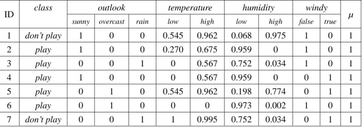
Now, we will use a training set as example to illustrate the learning process. The training set is shown in Table I. The data set is a mixed-mode data [15], [16], and there are four attributes, namely outlook, temperature, humidity, and wind. The decision classes are don’t play golf and play golf. In this example, the fuzzy sets of the continuous attributes are defined by genetic algorithm [17] that we will describe in the following section. The small training set with fuzzy representation is shown in Table II.

TABLE I

EXAMPLES OF TRAINING SET

ID Class outlook temperature humidity windy u

1 don’t play sunny 72 95 false 1

2 play sunny 69 70 false 1

3 play rain 75 80 false 1

4 play sunny 75 70 true 1

5 play overcast 72 90 true 1

6 play overcast 81 75 false 1

7 don’t play rain 71 80 true 1

TABLE II

EXAMPLES WITH FUZZY REPRESENTATION OF TRAINING SET

outlook temperature humidity windy

ID class

sunny overcast rain low high low high false true µ

1 don’t play 1 0 0 0.545 0.962 0.068 0.975 1 0 1 2 play 1 0 0 0.270 0.675 0.959 0 1 0 1 3 play 0 0 1 0 0.567 0.752 0.034 1 0 1 4 play 1 0 0 0 0.567 0.959 0 0 1 1 5 play 0 1 0 0.545 0.962 0.198 0.774 0 1 1 6 play 0 1 0 0 0 0.973 0.002 1 0 1 7 don’t play 0 0 1 1 0.995 0.752 0.034 0 1 1

From the theory we discuss above, we have D =7, ììDCdon0t playìì=2 and ìì_DCplayìì_{=5, we} have I(D)＝ 7 5 log 7 5 7 2 log 7 2 2 2 − − ＝0.863.

For “outlook,” we have

Doutlook,sunny

| | =3, ììDdon_{outlook,sunny}0t play ììì = ìì1, ìDplay_{outlook,sunny}ììì=2, I(Doutlook,sunny) =

ì

and 0.918;

Doutlook,overcast

| | =2, Ddon_{outlook,overcast}0t play 0, =2, ì Dplay_{outlook,overcast} ì ì ì ì_{ìì = ìì ìì} I(Doutlook,overcast) = ì ì_{ìì = ìì ìì} I(Doutlook,rain) = ì and 0; Doutlook,rain

| | =2, ì_ìDdon_outlook,rain0t play 1, ìDplay_outlook,rainì=1,

and 1.

Now we can calculate the entropy of the branch “outlook” as

E(outlook, D) = 1 7 2 0 7 2 918 . 0 7 3_{× + × + ×} ＝0.679. For “temperature,” we have

=

low e temperatur

D _, 2.36, _|Ddon_{temperature,low}0t play _{| =1.545, |D}play_{temperature,low| =}0.815, and I(Dtemperature,low) =0.93;

|Dtemperature,high| =4.728, |D

don0_{t play}

temperature,high| =1.957, |D 2.771, play

temperature,high| =

and I(Dtemperature,high) =0.979.

We can calculate the entropy of the branch “temperature” as

E(temperature, D) = 0.979 638 . 6 728 . 4 93 . 0 638 . 6 36 . 2 × + × . =1.028.

For “humidity,” we have |Dhumidity,low| =4.661, |D don0_{t play} humidity,low| =0.82, |D 3.841, play humidity,low| =

and I(Dhumidity,low) =0.671; |Dhumidity,high| =1.819, |Ddon

0_{t play}

humidity,high| =1.009, |D 0.81, play

humidity,high| =

and I(Dhumidity,high) =0.991; E(humidity, D) =0.761. For “wind,” we have

|Dwindy,false| =4, |D

don0_{t play}

windy,false| =1, |D 3, play

windy,false| =

and I(Dwindy,false) =0.811;

|Dwindy,true| =3, |Ddon 1, 2,

0_{t play}

windy,true| = |D play

windy,true| =

and I(Dwindy,true) =0.918; E(windy, D) =0.857.

Thus we have the information gain for the attribute “outlook” as

) , ( ) ( ) , (outlook D I D E outlook D G = − =0.863－0.679 =0.184.

By the same method for “temperature,” “humidity,” and “windy,” we have G(temperature, D) = à0.165, G(humidity, D) =0.102,

and G(windy, D) =0.006.

Now, we assign the order of features from the top to the bottom of the decision tree according to of features in decreasing order. Then the order of features is {outlook, humidity, windy, temperature}.

2.3. Tree Construction

In Fuzzy ID3 algorithm, we assign each example a unit membership value. Assume that we have a set of training data , where each data has continuous attributes and one classified class

D l

l

A A

A₁, ₂,..., C ={C1,C2,...,Cn} and fuzzy sets

for the attribute . Let be a fuzzy subset in whose class is

im i

i F F

F₁ , ₂ ,..., A_i DCk D

Ckand is the sum of the membership values in a fuzzy set of training data .

An algorithm to generate a fuzzy decision tree [2], [9] is shown in the following:

|D| D

1 ) Generate the root node and that has a set of all data, i.e., a fuzzy set of all data point with the unit membership value.

2 ) If a node with a fuzzy set of data t D satisfies the following conditions:

2.1 ) the proportion of a data set of a class is greater than or equal to a threshold , that is,

Ck òr _|D| |DCk_| , (2.6) õ òr

2.2 ) the number of a data set is less than a threshold òn, that is,

. |D| < òn, (2.7) 2.3 ) there are no attributes for more classifications, then it is a leaf node,

and we record the certainties

|D|

|D

Ck

_|

with all classes at the node.

3 ) If it does not satisfy the above conditions, it is not a leaf node, and the branch node is generated as follows:

3.1 ) Divide into fuzzy subsets according to the feature

D D1 ,D2 ,...,Dm

nodes. The membership value of example in is the product of the membership value in and the value of F of the value of

Dj

D ij

Ai in D.

3.2 ) Generate new nodes for fuzzy subsets

and label the fuzzy sets to edges that connect between the nodes and t . m t t t₁, ₂ ,..., D₁ ,D₂ ,...,D_m Fij j t

3.3 ) Select the next feature for generating the son nodes by the result of feature ranking.

4) Replace D by D and repeat from step 2 ) recursively until the end of all paths are leaf nodes.

j

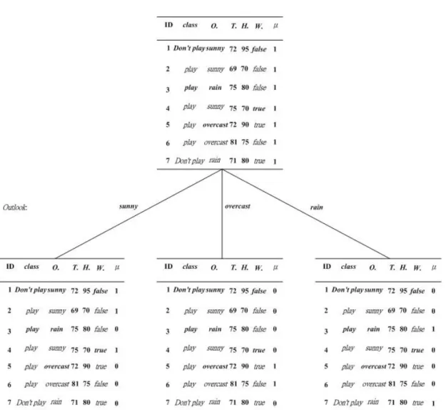
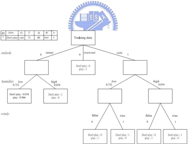
Now, we make the first layer of decision tree with the attribute “outlook” as shown in Fig. 2.1. There are three branches “sunny,” “overcast,” and “rain” from the root. We continue the construction process to produce the full fuzzy decision tree with other attributes until it satisfies the leaf node criterions above. For this training data, the fuzzy decision tree is shown in Fig. 2.2.

Fig. 2.2. The full fuzzy decision tree of this example.

2.4. Inference of Fuzzy Decision Tree

After generating the fuzzy decision tree from the training data , we need a method to test the classification of training examples or to predict the classification of other examples. At all the leaf nodes, we have recorded the certainties

D

|D| |DCk|

of each class as mentioned above. The rule produced by each leaf node which can classify the data point to each class with the certainty value. Then the reasoning by fuzzy decision

tree can be converted into a set of fuzzy rules. For example, the fuzzy rule extracted from the leaf node can be described as

IF outlook is sunny AND humidity is low

THEN don’t play with certainty 0.034 and play with certainty 0.966.

For the generated fuzzy decision tree, each connection from root to leaf is called path. There are one or more membership values between root and each leaf node because a continuous attribute value has a membership value according to the corresponding membership function. Assume that the fuzzy decision tree contains r

leaf nodes, and decision class. The steps to classify a data using obtained fuzzy rule base are described as follows:

n

1 ) For each (i 1_{ô i ô r}), the certainty of class j of the leaf node i

multiplied by the membership values which are on the path . Sum the terms to get which is the possibility of the class

i r

( )

j

P j.

2 ) Repeat from step 1 ) for each j (1 ) such that all the have been computed.

ô j ô n P

( )

j

3 ) The example e is assigned to the class which has the maximum value in

step 2 ).

An illustration is shown in Fig. 2.3, where the 7-th example of Table I is tested by the fuzzy rule-base. Thus we can use these 7 rules to classify the 7-th example of Table I as follows:

(

dont play

)

P ' = 0×0.752×0.034 + 0×0.034×1 + 0×0 + 1×0.752×0×0 + 1×0.752×1×1 + 1×0.034×0×0 + 1×0.034×1×1 = 0.786,

(

play

)

P = 0×0.752×0.966 + 0×0.034×0 + 0×1 + 1×0.752×0×1 + 1×0.752×1×0 + 1×0.034×0×0 + 1×0.034×0 = 0.

The 7-th example is assigned to class don’t play because is maximum between all the . Note that each rule has influence on the testing, so we use all rules to classify an example but not just depend on a single rule.

(

dont play

)

P '

( )

j P

2.5. Genetic Algorithm for Fuzzy ID3

From the description above, ò , and the membership functions of all the continuous features of Fuzzy ID3 algorithm are defined by a user. A good selection of fuzzy rule base, ò , and the membership functions are best matched to the database to be processed, would greatly improve the accuracy of the decision tree. To this end, any optimization algorithms seem appropriate for this purpose. In particular, genetic algorithm (GA) based scheme is highly recommended since a gradient computation for conventional optimization approach is usually not feasible for a decision tree. This is because condition-based decision path is nonlinear in nature, and hence its gradient is not defined. Based on the concept, we will introduce genetic algorithm to search best , and the membership functions of all the continuous features for the design of fuzzy ID3.

r, òn

r, òn

ò_r, ò_n

GA is adaptive heuristic search method that may be used to solve all kinds of complex search and optimization problems. It is an optimization search mechanism based natural selection process. Its essential mind is to imitate the criterion “survival of the fittest” of the biology. GA is often capable of finding optimal solutions even in the most complex of search spaces or at least it offer significant benefits over other search and optimization techniques. A typical GA operates on a population of solutions within the search space. The search space represents all the possible solutions that can be obtained for the given problem and is usually very complex or even infinite. Every point of the search space is one of the possible solutions and therefore the aim of the GA is to find an optimal point or at least come as close to is as possible.

The advantage of GA is in their parallelism. GA is considering many individuals instead of an individual in a search space. It gets the global optimum rapidly, furthermore avoids the chance to fall into the local optimum.

GA is typically implemented as a computer simulation in which a population of chromosomes of individuals to an optimization problem evolves toward better solutions. Traditionally, solutions are represented in binary as strings of 0s and 1s, but different encodings are also possible. In this thesis, we use 6-bits to represent a parameter. We use GA to tune the thresholds ò , and the parameters of the membership functions of feature values. The membership function of each sub-attribute is assumed to be Gaussian-type and is given by

r, òn

m(x) = exp

(

à

2û

2

(x

_àö)

2

)

_{, (2.8)}

where x is the corresponding feature value of the data point with mean ö and standard deviation . Thus for each membership function, we have two parameters û

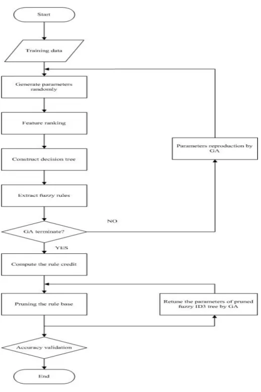
ö and û to tune. For example, assume we have a data set, which has 4 continuous attributes and 3 classes such that there are 12 membership functions. Each membership function has 2 parameters and there are 2 thresholds of leaf condition in addition. Thus we have 26 parameters to be tuned, and the length of a binary chromosome is 156. There are three operators of genetic algorithm which are reproduction, crossover, and mutation. We briefly describe how to perform these three operators. The flowchart of GA is shown in Fig. 2.4.

Fig. 2.4. Flowchart of genetic algorithm.

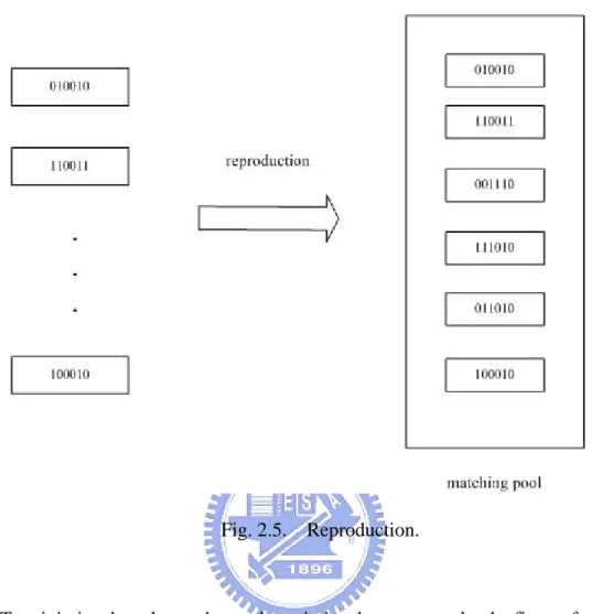
Reproduction is a process according to the fitness degree of each individual to decide which will be eliminated or copied at next generation, the individual with higher fitness value will be copied in a large number; the individual with lower fitness value will be eliminated. The potential chromosomes of the population are copied into a mating pool depending on their fitness values. The operator is shown in Fig. 2.5.

Fig. 2.5. Reproduction.

To minimize the rule number and maximize the accuracy, let the fitness function

(

)

(

)

(

Ai Aworst Ravg Ri

f =100100 − 2+

)

, (2.9) where is the learning accuracy of the individual , and is the worst learning accuracy of all individuals. is the average number of the rules of all individuals, and is the number of the rules of the individual .

i A i A_worst avg R i R i

Crossover is a process with selecting two potential chromosomes randomly from the matching pool, and exchange bit information mutually to produce two new individuals. Roughly speaking, it hopes to generate greater filial generation by accumulating the superior bit information of parents. An example for crossover is shown as Fig. 2.6.

Fig. 2.6. Crossover.

Mutation is an occasional alteration of a random bit. It is the process that selects randomly string of an individual and selects randomly the mutation point to change the bit information of the string. The probability of this process is controlled by the mutation probability. For binary string, “0” is changed to “1,” and “1” is changed to “0.” The mutation is shown as Fig. 2.7. Mutation that helps to find an optimal solution to the given problem more reliably, as it prevents GA from finishing the search prematurely with a sub-optimal solution.

Fig. 2.7. Mutation.

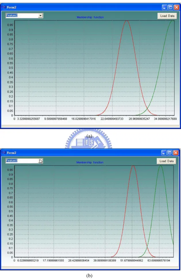
After the genetic algorithm above, the system will generate two parameters of Gaussian-type membership function ö and û, and we get the parameters 0.827, and 0.001 of the criterions for tree construction. The membership functions of each continuous attribute for the training set are illustrated in Fig. 2.8.

òr=

(a)

(b)

Fig. 2.8. The membership functions of each attribute for the training set. (a) The membership functions of “temperature.” (b) The membership functions of “humidity.”

Chapter 3. Pruning Methods for Fuzzy ID3

3.1. Introduction of Pruning Method

There are many pruning methods which can be grouped into two classes: pre-pruning and post-pruning. The former approaches stop growing the tree earlier, before it reaches the point where it perfectly classifies the training data, and the other approaches that allow the tree to ovefit the data, and then post-prune it. Although the first kind of approaches might seem more direct, the second kind of approaches of post-pruning has been found to be more successful in practice. The reason involves that pre-pruning methods have difficulty in estimating precisely when to stop growing the tree. Moreover, a very important benefit of post-pruning methods is that they can generate a sequence of trees instead of a single one, which allows expert to seek the optimal one out based on his professional knowledge. In this thesis, we propose to adopt the post-pruning method for our study.

For the generation of fuzzy decision trees, the tree size is a very important issue. The aim of pruning is to reduce the number of nodes while the accuracy is retained. In this thesis, we propose to use mathematical method to investigate how the rules of pruning algorithms influence fuzzy decision trees.

3.2. Description of Our Pruning Methods

We have used the GA to improve the performance of the classification task and decrease the rule number as well. In this thesis, we propose three pruning methods to

further minimize the number of rules. The first pruning method is described as follows:

1 ) For each rules, when any data point is classified, we maintain the production value of the membership value and the certainty of each class,

, where n is an index of each class.

) (n

J

2 ) corresponding to the correct class of the data point gets positive sign and the others get negative sign.

) (n

J

3 ) Sum for all classes of , and then we get the credit of the rule to classify this data point.

... ), 2 ( ), 1 ( J J J(n)

4 ) Repeat from 1) until all data points are classified by this rule and we get the final credit of this rule.

5 ) Remove the redundant rules whose the credits are less than certain threshold and/or have big drops.

In the second pruning method, when any data point is classified, we define the

second credit formula 2 as

j V

(

)

2 1 2 2 1 1 2 1 p p c r r r V c j c j j j j j j ₋ − + + − = α α α L , (3.1)

where c is the class number of the training data, is the production value of the membership value which corresponds to the maximum possibility of the class for the

j-th rule; is the possibility ratio assigned to the maximum class of the j-th rule.

And is the production value of the membership value which corresponds to the

1 j α 1 j r 2 j α

second largest possibility of the class for the j-th rule, and is the possibility ratio

assigned to the second largest class for the j-th rule; other and follow similarly. Value is the maximum possibility of the class which is the sums of each class assigned by each rule; is the second largest possibility of the class which is the sums of each class assigned by each rule. The credit value gets positive sign when the class of the and is the same. On the contrary, if the class of

the and is different, the credit value gets negative sign. If the is equal to

the , the credit value is assigned to 10000. Instead of ,

2 j r ∗ j α ∗ j r 1 p 2 p 1 j α 1 p 1 j α 1 p p1 2 p 2 j V p2 p2_c−1 may be another solution.

The third pruning method is improved from the second kind of the pruning method. We revise the third credit formula 3 as

j V 2 1 2 1 3 p p V _j j j − − = α α _{, (3.2)}

where is the production value of the membership value which corresponds to the

maximum possibility of the class for the j-th rule, is the production value of the membership value which corresponds to the second largest possibility of the class for the j-th rule. Value is the maximum possibility of the class which is the sums of each class assigned by each rule, is the second largest possibility of the class which is the sums of each class assigned by each rule. The credit value gets positive sign when the class of the and is the same. On the contrary, if the class of

the and is different, the credit value gets negative sign. If the is equal to

1 j α 2 j α 1 p 2 p 1 j α 1 p 1 j α 1 p p1

the p2, the credit value 3 is assigned to 10000. Instead of , j V p2 ₁ 2 − c p _{may be} another solution.

The credit of each rule computed and then arranged in an order of from the largest to the smallest. This number represents the effectiveness of the rule in performing the classification task. If the rule is essential for classification, then it would get a high credit value. On the contrary, if the credit is low, this rule could be an insignificant or redundant rule. The reason is explained as follows. The rule that classifies the instance to the true class or to the wrong class will be cumulatively counted. In this way, we can prune the insignificant or inconsistent rules to obtain a smaller and efficient rule base set. After deleting the inefficient rule or rules, we retune the parameters of pruned Fuzzy ID3 tree again by GA.

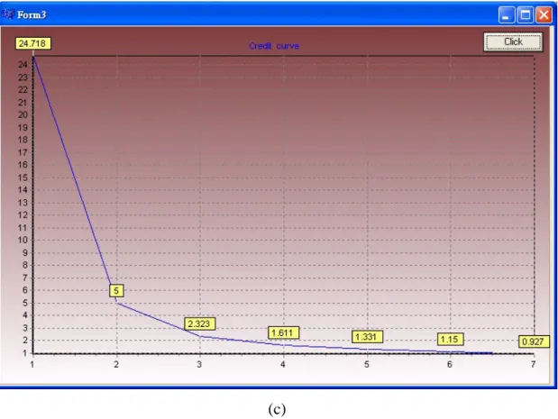
For example, after we get the credit of each rule of the training set as shown in Table I, we then sort and plot the total credit of all rules of each credit computation of the above three pruning methods. They are as shown in Figs. 3.1(a)–(c), respectively. We find that the credit of the 6-th rule and 7-th rule are much smaller than others, which indicates that these two rules may be redundant. Hence, we can select the following thresholds: (a) between 1 and 0.589; (b) between 0.645 and 6.965; (c) between 1.331 and 1.15, for these three methods, respectively, and remove the redundant rules. The pruned fuzzy decision trees of the training set as shown in Table I, are shown in Fig. 3.2(a)–(c), respectively. The flowchart of our genetic algorithm based fuzzy ID3 method is illustrated in Fig. 3.3.

(a)

(c)

Fig. 3.1. The credit plot on each rule: (a) result of the first pruning method, (b) result of the second pruning method, and (c) result of the third pruning method.

(a)

(c)

Fig. 3.2. Fuzzy decision trees after pruning: (a) result of the first pruning method, (b) result of the second pruning method, (c) result of the third pruning method.

Chapter 4. Simulation and Experiment

As mentioned in Chapter 2, we introduce a fuzzy ID3 algorithm to construct a fuzzy classification system whose membership functions and leaf conditions are tuned by GA. In this chapter, we apply the algorithm to classify some data sets, which include continuous, discrete, and mixed-mode data sets [14], [16]. We also use this method together with three pruning methods to classify these data sets and compare the results. This simulation was done on Pentium 4 CPU 3.4 GHz personal computers with 2GB RAM.

4.1. Description of The Data Sets

The ten well known data sets employed for experiments are obtained from the University of California, Irvine, Repository of Machine Learning databases (UCI) [20]. Their characters are briefly described below.

1 ) Crude_oil: Gerrid and Lantz analyzed Crude_oil samples from three

zones of sandstone. The Crude_oil data set with 56 examples has five attributes and three classes named wilhelm, submuilinia, and upper. The attributes are vanadium (in percent ash), iron (in percent ash), beryllium (in percent ash), saturated hydrocarbons (in percent area), and aromatic hydrocarbons (in percent area).

2 ) Glass Identification Database: The data set represents the problem of

identifying glass samples taken from the scene of an accident. The 214 examples were originally collected by B. German of the Home Office

Forensic Science Service at Aldermaston, Reading, Berkshire in the UK. The nine attributes are all real valued and fully known, representing refractive index and the percent weight of oxides such as silicon, sodium, and magnesium. The six classes are named as building windows float processed, building windows not float processed, vehicle windows float processed, containers, tableware, and headlamps

3 ) Iris Plant Database: The Iris data set, Fisher’s classic test data (Fisher,

1936), has three classes with four-dimensional data consisting of 150 examples. The four attributes are: sepal length, sepal width, petal length, and petal width. This data set gives good results with almost all classic learning methods and has become a sort of benchmark data.

4 ) Myo_electric: The Myo_electric data set is extracted from a problem in

discriminating between electrical signals observed at the human skin surface. This is a four-dimensional data set consisting of 72 examples divided into two classes.

5 ) Norm4: The data set has 800 examples consisting of 200 examples each

from the four components of a mixture of four class 4-variate normals.

6 ) BUPA liver disorders: This UCI data set was donated by R. S. Forsyth.

The problem is to predict whether or not a male patient has a liver disorder based on blood tests and alcohol consumption. There are two classes, six continuous attributes, and 345 examples.

7 ) Promoter Gene Sequences Database: Promoters have a region where a

protein (RNA polymerase) must make contact and the helical DNA sequence must have a valid conformation so that the two pieces of the contact region spatially align. The data set with 106 examples has 57 attributes and two classes. All attributes are discrete.

8 ) StatLog Project Heart Disease dataset: This UCI data set is from the

Cleveland Clinic Foundation, courtesy of R. Detrano. The problem concerns the prediction of the presence or absence of heart disease given the results of various medical tests carried out on a patient. There are two classes, seven continuous attributes, six discrete attributes, and 270 examples.

9 ) Golf: The data set with 28 examples has four attributes and two classes

named play, and don’t play. There are 2 continuous and 2 discrete attributes. The attributes are outlook, temperature, humidity, and windy. 10) StatLog Project Australian Credit Approval: This credit data originates

from Quinlan. This file concerns credit card applications. All attribute names and values have been changed to meaningless symbols to protect confidentiality of the data. The Australian data set with 690 examples has 14 attributes and two classes. There are 6 continuous and 8 discrete attributes.

In older to clearly summarize the ten data sets, we list the properties of them in Table Ⅲ and the partial examples of our testing data sets are illustrated in Fig. 4.1.

TABLE III

S

UMMARY OF THE

D

ATABASES

E

MPLOYED

Data set # of examples # of attributes # of continuous

attributes # of classes Crude oil 56 5 5 3 Glass 214 9 9 6 Iris 150 4 4 3 Myo_electric 72 4 4 2 Norm4 800 4 4 4 Bupa 345 6 6 2 Promoters 106 57 0 2 Heart 270 13 6 2 Golf 28 4 2 2 Australian 690 14 6 2

4.2. Simulation and Comparison

We use all the data sets to be the training data and the same examples to be the testing data for the performance evaluation with our proposed GA based fuzzy ID3 method. In rule pruning, we remove the redundant rules that will still maintain or only slightly reduced the learning accuracy to be considered as acceptable. We take down the accuracy and the number of fuzzy rules before and after pruning. We have applied three pruning methods; their results are shown in Tables IV, V, and VI, respectively. For classifying Glass data set, we consider only five attributes that are Na, Mg, Al, K, Ba according to feature subset select [21]. In addition, we divide the sub-feature into two partitions for Norm4, and divide three partitions for Glass. If we do not reduce the attributes of this data set, we will obtain too many rules after tree construction. Without the restrictions above, the fuzzy ID3 still can not increase in the learning accuracy.

TABLE IV

P

ERFORMANCE OF THE

D

ATA

S

ETS BEFORE AND AFTER

P

RUNING BY THE

F

IRST

P

RUNING

M

ETHOD

Before rule pruning After rule pruning Data set

# of rules Training acc. # of rules Training acc.

Crude_oil 13.0 100.0 8.0 97.7 Glass 11.0 75.4 9.0 69.0 Iris 4.0 99.1 3.0 97.5 Myo_electric 4.0 96.4 3.0 92.9 Norm4 5.0 93.9 4.0 72.0 Bupa 8.0 76.8 7.0 76.8 Promoters 10.0 85.7 8.0 85.7 Heart 15.0 87.0 13.0 86.1 Golf 6.0 95.4 5.0 95.4 Australian 4.0 86.4 2.0 87.3

TABLE V

P

ERFORMANCE OF THE

D

ATA

S

ETS BEFORE AND AFTER

P

RUNING BY THE

S

ECOND

P

RUNING

M

ETHOD

Before rule pruning After rule pruning Data set

# of rules Training acc. # of rules Training acc.

Crude_oil 13.0 100.0 12.0 97.7 Glass 11.0 75.4 10.0 73.6 Iris 4.0 99.1 3.0 91.6 Myo_electric 4.0 96.4 3.0 92.9 Norm4 5.0 93.9 4.0 83.9 Bupa 8.0 76.8 6.0 77.1 Promoters 10.0 85.7 4.0 84.5 Heart 15.0 87.0 4.0 79.1 Golf 6.0 95.4 3.0 95.4 Australian 4.0 86.4 2.0 87.3

TABLE VI

P

ERFORMANCE OF THE

D

ATA

S

ETS BEFORE AND AFTER

P

RUNING BY THE

T

HIRD

P

RUNING

M

ETHOD

Before rule pruning After rule pruning Data set

# of rules Training acc. # of rules Training acc.

Crude_oil 13.0 100.0 10.0 100.0 Glass 11.0 75.4 8.0 74.8 Iris 4.0 99.1 3.0 97.5 Myo_electric 4.0 96.4 3.0 92.9 Norm4 5.0 93.9 4.0 92.8 Bupa 8.0 76.8 5.0 76.8 Promoters 10.0 85.7 5.0 84.5 Heart 15.0 87.0 11.0 86.1 Golf 6.0 95.4 4.0 95.4 Australian 4.0 86.4 2.0 87.5

From Tables IV, V, and VI, we find that most of data sets slightly reduce the accuracy after rule pruning. This has happened possibly because the rule pruning process has removed some rules, which were correctly classifying these data sets. And the residual rules are not able to correctly classify few examples. We can also see that the number of the rules is decreased for all data sets, which shows the effectiveness of our rule pruning process.

From Table VII, we compare the accuracy with different pruning methods for each data set; moreover, we can find that for Myo_electric and Golf data sets, the accuracy have the same with different pruning method. For the others except Promoters data, the third pruning method is superior to others in accuracy. Table VIII compares the number of rules with different pruning methods for each data set. We can find that for Iris, Myo_electric, and Norm4 data sets, the number of rules is the same with different pruning method. For the others expect Crude_oil, Glass, and Bupa, the second pruning method is smaller than others in the number of rules.

TABLE VII

C

OMPARISON OF THE

A

CCURACIES WITH

D

IFFERENT

P

RUNING

M

ETHODS

After rule pruning

First Pruning Second Pruning Third Pruning Data set

Training acc. Training acc. Training acc.

Crude_oil 97.7 97.7 100.0 Glass 69.0 73.6 74.8 Iris 97.5 91.6 97.5 Myo_electric 92.9 92.9 92.9 Norm4 72.0 83.9 92.8 Bupa 76.8 77.1 76.8 Promoters 85.7 84.5 84.5 Heart 86.1 79.1 86.1 Golf 95.4 95.4 95.4 Australian 87.3 87.3 87.5

TABLE VIII

C

OMPARISON OF THE

N

UMBER OF

R

ULES WITH

D

IFFERENT

P

RUNING

M

ETHODS

After rule pruning

First Pruning Second Pruning Third Pruning Data set

# of rules # of rules # of rules

Crude_oil 8.0 12.0 10.0 Glass 9.0 10.0 8.0 Iris 3.0 3.0 3.0 Myo_electric 3.0 3.0 3.0 Norm4 4.0 4.0 4.0 Bupa 7.0 6.0 5.0 Promoters 8.0 4.0 5.0 Heart 13.0 4.0 11.0 Golf 5.0 3.0 4.0 Australian 2.0 1.0 2.0

For classifying system, the main concern is its accuracy; therefore, we compare performance with the best two pruning methods, i.e., the first and third second pruning method further. We use five-fold cross validation testing which divides the each data set into five folds. Namely, the instances are randomly divided among the five folds. The first fold is the testing data, the others are used for training. Then the learned structure is then tested against the first fold. The same procedure is repeated considering the second fold to be the testing data and the others to be the training data, the procedure is operated until the fifth fold. Average accuracy and the number of rules are recorded in Tables IX and X, respectively. This procedure is repeated three times.

Table IX shows the comparison of the accuracies of the first pruning and the third pruning methods. On average, we find that for Heart data set, the accuracy of the first pruning and second pruning are the same. For the others, the third pruning method outperforms the first pruning method in accuracy. Similarly, Table X shows that the rule number of the third pruning method is smaller than that of the first pruning method. Finally, for our proposed GA based fuzzy ID3 with third pruning method is compared to C5.0 [6]. The reason why we choose C5.0 is that C5.0 is a decent version of C4.5 and is the state-of-the-art algorithm, which works well for many decision-making problems.

TABLE IX

C

OMPARISON OF THE

T

ESTING

A

CCURACIES WITH

T

WO

B

ETTER

P

RUNING

M

ETHODS

Testing acc. (five-fold CV repeated three times) Data set Pruning Method

1 2 3 Avg. acc. First Pruning 75.8 89.1 83.3 82.7 Crude_oil Third Pruning 78.3 90.8 85.0 84.7 First Pruning 54.8 56.2 48.3 53.1 Glass Third Pruning 62.3 58.1 56.2 58.9 First Pruning 93.3 91.3 88.0 90.9 Iris Third Pruning 93.3 92.7 90.6 92.2 First Pruning 78.6 73.6 77.6 76.6 Myo_electric Third Pruning 90.3 79.6 81.0 83.6 First Pruning 86.6 77.2 74.2 79.3 Norm4 Third Pruning 86.5 82.7 73.7 81.0 First Pruning 64.3 66.0 58.2 62.8 Bupa Third Pruning 64.3 66.3 62.9 64.5 First Pruning 80.0 78.6 73.3 77.3 Promoters Third Pruning 80.3 76.7 75.1 77.4 First Pruning 74.8 72.5 67.7 71.7 Heart Third Pruning 74.8 72.5 67.7 71.7 First Pruning 86.6 83.3 86.6 85.5 Golf Third Pruning 93.3 93.3 93.3 93.3 First Pruning 84.7 85.1 83.6 84.5 Australian Third Pruning 84.3 85.6 84.9 84.9

TABLE X

C

OMPARISON OF THE

N

UMBER OF

R

ULES WITH

T

WO

B

ETTER

P

RUNING METHODS

# of rules (five-fold CV repeated three times) Data set Pruning Method

1 2 3 Avg. rules First Pruning 7.6 11.6 9.8 9.7 Crude_oil Third Pruning 9.2 12.6 9.8 10.5 First Pruning 12.0 13.8 12.2 12.7 Glass Third Pruning 11.8 14.0 11.6 12.5 First Pruning 5.2 3.8 5.2 4.7 Iris Third Pruning 4.6 3.4 4.6 4.2 First Pruning 2.8 2.0 2.6 2.5 Myo_electric Third Pruning 3.0 2.2 2.6 2.6 First Pruning 4.6 4.2 4.0 4.3 Norm4 Third Pruning 4.4 4.2 3.4 4.0 First Pruning 6.2 4.4 6.6 5.7 Bupa Third Pruning 5.8 3.8 5.8 5.1 First Pruning 8.2 6.6 3.6 6.1 Promoters Third Pruning 6.8 7.0 2.8 5.5 First Pruning 5.2 8.0 5.0 6.1 Heart Third Pruning 4.6 7.0 3.0 4.9 First Pruning 5.0 5.2 4.0 4.7 Golf Third Pruning 3.6 5.2 5.8 4.9 First Pruning 1.4 1.2 1.6 1.4 Australian Third Pruning 1.6 1.4 1.2 1.4

Accuracy comparison result of our method to C5.0 is shown in Table XI. It records the testing accuracy from five-fold cross validation, repeated three times on each data set. On average, we find that our rule-base outperforms C5.0 in seven out of ten data sets. Thus our system has better generalization ability than C5.0. Our method is also compared to C5.0 with respect to the average number of rules. Table XII shows the comparison of the number of rules generated by these two methods at the same experiment. The training time and executive time of our method for the data sets, are recorded in Table XIII. This simulation was done on Pentium 4 CPU 3.4 GHz personal computers with 2GB RAM. The training and executive time for C5.0 are very fast, less than 0.1 sec., for all the above data sets. We find that our rule-base is smaller than C5.0 in seven out of ten data sets. It is evident that our approach tends to produce a better classification accuracy with more concise rule sets than C5.0.

TABLE XI

A

CCURACY

C

OMPARISON OF

O

UR

M

ETHOD AND

C5.0

Testing acc. (five-fold CV repeated three times) Data set Algorithm

1 2 3 Avg. acc. Our rule-base 78.3 90.8 85.0 84.7 Crude_oil C5.0 72.5 79.2 76.7 76.1 Our rule-base 62.3 58.1 56.2 58.9 Glass C5.0 62.8 65.6 69.8 66.0 Our rule-base 94.0 96.0 96.0 95.3 Iris C5.0 93.4 95.3 96.7 95.1 Our rule-base 94.6 87.3 94.3 92.1 Myo_electric C5.0 89.0 91.6 82.0 87.5 Our rule-base 92.0 92.6 92.8 92.5 Norm4 C5.0 92.5 91.0 92.6 92.0 Our rule-base 64.6 66.6 64.3 65.2 Bupa C5.0 65.8 60.3 65.5 63.9 Our rule-base 80.3 76.6 75.1 77.3 Promoters C5.0 80.3 76.5 70.6 75.8 Our rule-base 77.7 73.3 70.3 73.8 Heart C5.0 79.3 75.5 76.8 77.2 Our rule-base 93.3 96.7 93.3 94.4 Golf C5.0 86.7 96.7 96.6 93.3 Our rule-base 84.3 85.8 85.2 85.1 Australian C5.0 84.8 86.2 86.0 85.7

TABLE XII

R

ULE

N

UMBER

C

OMPARISON OF

O

UR

M

ETHOD AND

C5.0

# of rules (five-fold CV repeated three times) Data set Algorithm

1 2 3 Avg. rules Our rule-base 9.2 12.6 9.8 10.5 Crude_oil C5.0 4.6 4.4 4.6 4.5 Our rule-base 11.8 14.0 11.6 12.5 Glass C5.0 15.0 13.0 16.0 14.7 Our rule-base 4.8 3.6 6.0 4.8 Iris C5.0 4.0 3.8 4.2 4.0 Our rule-base 3.4 2.8 3.6 3.3 Myo_electric C5.0 4.4 3.8 3.8 4.0 Our rule-base 5.0 4.6 5.0 4.9 Norm4 C5.0 19.0 18.4 15.8 17.8 Our rule-base 6.0 3.8 6.0 5.3 Bupa C5.0 15.2 17.4 20.8 17.8 Our rule-base 6.8 7.0 2.8 5.5 Promoters C5.0 12.6 12.6 12.0 12.4 Our rule-base 5.0 7.6 3.2 5.3 Heart C5.0 18.2 18.4 21.2 19.3 Our rule-base 3.6 5.4 5.8 4.9 Golf C5.0 5.2 4.2 5.0 4.8 Our rule-base 1.6 2.2 1.8 1.9 Australian C5.0 17.0 11.4 17.0 15.1

TABLE XIII

T

RAINING

T

IME AND

E

XECUTIVE

T

IME OF

O

UR

M

ETHOD

Data set Training Time (sec) (five-fold CV)

Executive Time ( sec) (five-fold CV) 3 10− × Crude_oil 0.203 1.433 Glass 1.591 0.651 Iris 0.172 0.526 Myo_electric 0.156 1.107 Norm4 0.114 0.098 Bupa 0.422 0.269 Promoters 0.024 5.650 Heart 0.362 0.411 Golf 0.289 3.134 Australian 0.407 0.115

Chapter 5. Conclusion

In this thesis, we proposed a genetic algorithm based fuzzy ID3 method to construct fuzzy classification system, which can accept continuous, discrete, or mixed-mode data sets. Next, we formulated three pruning methods to obtain a more efficient rule base. In the experiment, we found that the third pruning method was superior to the others; therefore, we used genetic algorithm based fuzzy ID3 with the third pruning method to classify data. Our proposed method can directly classify mixed-mode data set with high classification accuracy. On testing to some famous data sets, which include continuous, discrete, and mixed-mode data sets, we have obtained a very high classification accuracy with small number of rules. It is remarked that the decision tree after pruning can lead to a smaller fuzzy rule base and the pruned rule base can usually remain or decrease slightly the classification performance despite the deduction of the number of the rules.

Furthermore, on comparing the results generated by our proposed method with C5.0, we find that our rule-base outperforms C5.0 in seven out of ten data sets. As demonstrated in the testing, the proposed new pruning method is helpful to improve the testing accuracy.

For Heart, Australian, Myo_electric and Norm4 data sets, if the rule number of our fuzzy ID3 method is less than four, the accuracy is greatly decreased after pruning. In further work, when the rule number is few, we will determine whether the pruning method will be used or not. Computation consuming is another task in the field of

machine learning, we must try to reduce the computation burden in this scheme. These will be a good challenge to study in the future.

References

[1] E. Alpaydin, Introduction to Machine Learning. Cambridge, Massachusetts: MIT Press, 2004.

[2] Y. Yuan and M. J. Shaw, “Induction of fuzzy decision trees,” Fuzzy Sets Syst., vol. 69, pp. 125–139, 1995.

[3] M. S. Chen and J. Han, “Data mining: An overview from a database perspective,” IEEE Trans. Knowledge and Data Eng., vol. 8, no. 6, pp. 866–883, Dec. 1996.

[4] J. R. Quinlan, “Induction of decision trees,” Machine learning, vol. 1, pp. 81–106, 1986.

[5] J. R. Quinlan, C4.5, Programs for Machine Learning. San Mateo, CA: Morgan Kauffman, 1993.

[6] Data Mining Tools, http://www.rulequest.com/see5-info.html, 2003.

[7] L. Breiman et al., Classification and Regression Trees. Monterey, CA: Wadsworth and Brooks/Cole, 1984.

[8] M. Umano et al., “Fuzzy decision trees by fuzzy ID3 algorithm and its application to diagnosis systems,” in Proc. Third IEEE Conf. on Fuzzy Systems, vol. 3, pp. 2113–2118, 1994.

[9] C. Z. Janikow, “Fuzzy decision trees: issues and methods,” IEEE Trans. Syst.,

Man, Cybern. B, vol. 28, no. 1, pp. 1–14, Feb. 1998.

[10] X. Z. Wang et al., “On the optimization of fuzzy decision trees,” Fuzzy Sets Syst., vol. 112, pp. 117–125, 2000.

[11] I. Hayashi et al., “Generation of decision trees by fuzzy ID3 with adjusting mechanism of AND/OR operators,” in IEEE Int. Conf. Fuzzy Syst., Anchorage,

AK, pp. 681–685, May 1998.

[12] X. Z. Wang and J. R. Hong, “On the handling of fuzziness for continuous-valued attributes in decision tree generation,” Fuzzy Sets Syst., vol. 99, pp. 283–290, 1998.

[13] E. C. C. Tsang, X. Z. Wang, and D. S. Yeung, “Improving learning accuracy of fuzzy decision trees by hybrid neural networks,” IEEE Trans. Fuzzy Syst., vol. 8, no.5, pp. 601–614, Oct. 2000.

[14] J. Catlett, “On changing continuous attributes into ordered discrete attributes,” in

Proc. European Working Session on Learning, pp. 164–178, 1991.

[15] J. Y. Ching, A. K. C. Wong, and K. C. C. Chan, “Class-dependent discretization for inductive learning from continuous and mixed mode data,” IEEE Trans.

Pattern Analysis and Machine Intelligence, vol. 17, no. 7, pp. 641–651, July

1995.

[16] L. A. Kurgan and K. J. Cios, “CAIM discretization algorithm,” IEEE Trans.

Knowledge and Data Eng., vol. 16, no. 2, pp. 145–153, Feb. 2004.

[17] C. T. Lin and C. S. G. Lee, Neural Fuzzy Systems: A Neural-Fuzzy Synergism to

Intelligent Systems. Upper Saddle River, New Jersey: Prentice-Hall, 1996.

[18] N. R. Pal and S. Chakraborty, “Fuzzy rule extraction from ID3-type decision trees for real data,” IEEE Trans. Syst., Man, Cybern B, vol. 31, no. 5, pp. 745–754, Oct. 2001

[19] R. C. Gonzalez and R. E. Woods, Digital Image Processing, New Jersey, Prentice-Hall, 2002.

[20] C. Blake and E. K. Merz, UCI Repository of Machine Learning Database, 1998. [21] H. Wang, D. Bell, and F. Murtagh, “Axiomatic approach to feature subset

selection based on relevance,” IEEE Trans. Pattern Analysis and Machine