THE MAXIMUM BIT RATES OF SOLITON COMMUNICATION-SYSTEMS WITH LUMPED AMPLIFIERS AND FILTERS IN DIFFERENT DISTANCES

(1)

JOURNAL OF LIGHTWAVE TECHNOLOGY, VOL 13, NO 6, JUNE 1995 1121

The Maximum Bit Rates of Soliton

Communication Systems with Lumped

Amplifiers and Filters in Different Distances

Sien Chi, Jeng-Cherng Dung, and Senfar Wen

Abstract-The maximum bit rate of a soliton communication system with lumped amplifiers and optical filters is considered. When the dispersion of the fiber varies from one amplifier spacing to another amplifier spacing, the maximum bit rate is significantly reduced. To overcome the effect, the amplitude of the soliton is amplified so that it is still the average soliton corresponding to the fiber dispersion for an amplifier spacing. Thus, the maximum bit rate is only slightly less than that without the dispersion variations. For a given distance, the maximum bit rate limited by the stability and soliton interaction is obtained. The result is compared with that limited by the Gordon-Haus effect. For shorter transmission distance, the maximum bit rate is limited by the stability and soliton interaction. For longer transmission distance, the maximum bit rate is limited by the Gordon-Haus effect.

I. INTRODUCTION

OR long distance optical communication systems based

F

on the optical soliton, the dispersion is balanced by the nonlinear effect along the fiber [ 13. It is essential to amplify the soliton periodically to maintain its power. Stimulated Raman process has been proposed to amplify the solitons [2], [3]. Mollenauer and Smith have demonstrated that the solitons can transmit over 6000 km with Raman amplifiers by circulating the solitons in a fiber loop [4]. With the rapid development of the erbium-doped fiber amplifier (EDFA), it is used as a lumped amplifier to effectively amplify the solitons [5]-[7]. The required pump power is lower than that of the Raman amplifier. With the EDFA, the soliton power is amplified to an amplitude larger than the fundamental soliton power so that its average power along the fiber is still the fundamental soliton power [8]-[lo]. Such a soliton is called the average soliton, which is stable when the ratio of the amplifier spacing La and the soliton period z , is much less than unity. Since the soliton period is inversely proportional to the square of the pulsewidth, the soliton pulsewidth must be long enough to meet this requirement. however, this requirement is not necessary if the interested transmission distance is finite.

In addition to the stability requirement, there are two other effects limiting the capacity of soliton transmission. When the Manuscript received February 2, 1994; revised November 16, 1994. This work was supported in part by National Science Council, Republic of China, Contract NSC 83-0417-E-009-013.

S. Chi and J.-C. Dung are with the Institute of Electrical-Optical Engi- neering and Center for Telecommunications Research, National Chiao Tung University, Hsinchu, Taiwan 30050, R.O.C.

S. Wen is with the Department of Electrical Engineering, Chung-Hua Polytechnic Institute, Hsinchu, Taiwan, R.O.C.

IEEE Log Number 941 1567.

solitons are closely spaced, the mutual interaction changes the velocity of the solitons and causes the solitons to move out of the detection window. On the other hand, the noise introduced by the optical amplifier randomly modulates the carrier frequency of the soliton, and the group velocity varies. This effect leads to the timing jitter and is known as the Gordon-Haus effect [ 111. Both effects can be reduced by two methods. One is to use a Fabry-Perot filter after amplification [12]-[14]. The filter stabilizes the carrier frequency of the solitons, and both the velocity changes caused by the soliton interaction and amplifier noise can be reduced. The other is to control the timing of the solitons by synchronous modulation

[ 141-[ 171. Both methods have been demonstrated successfully, but the system with synchronous modulation is more complex. In fact, both methods can be combined to control the soliton. In this paper, for a given amplifier spacing and total transmission distance, the maximum bit rate of the system with Fabry-Perot filters is numerically studied. For the maximum bit rate, the stability, the soliton interaction, and the Gordon- Haus effect should be considered. However, it is complicated to consider the three effects simultaneously. We will consider the stability and the soliton interaction at the same time. The results are compared with the limits solely imposed by the Gordon-Haus effect. From the comparison, the parameters are re-adjusted so that the three limits can be met simultaneously. Here, we consider the scheme with optical filters to reduce the soliton interaction and Gordon-Haus effect. The filter bandwidth is optimized for the maximum bit rate. Furthermore, as the dispersion of the fiber can not be controlled perfectly, there are dispersion variations for the fibers. Such variations lead to similar effect as power variations because the power of the fundamental soliton depends on the fiber dispersion. It has been shown that the dispersion variations can be ignored when L a / z o

<<

1 [9]. Since we are interested in the maximum bit rate, where the values of L,/z, is not much less than unity, the dispersion variations may not be ignored. It will be shown that the dispersion variations seriously degrade the bit rate. To further improve the bit rate, the soliton power is amplified so that the average soliton is the corresponding fundamental soliton for the average dispersion of the fiber.

In Section 11, the theoretical model used in this paper is given. The high-order dispersion and the effect of self-frequency shift are considered because the interested pulsewidth is short. In Section 111, the maximum bit rate limited by the stability and soliton interaction for a given 0733-8724/95$04.00 0 1995 IEEE

(2)

obtained from Section I11 is compared with the maximum bit rate limited by the Gordon-Haus effect. The conclusion is given in Section V.

11. THEORETICAL MODEL

The soliton propagating in the fiber can be described by the modified nonlinear Schrodinger equation

where U, (, and r are the electric field envelope, distance, and time normalized to the electric field scale Q, dispersion length L D , and time scale To, respectively. Q, L o , and To are related by

27rc T,”

X2 D ( 2 4

LD =

--

where X is the operating wavelength, nz is the Kerr coefficient, A,R is the effective fiber cross section, and D is the dispersion parameter. The soliton period z, = (r/2)LD. The coefficients in (1) are

r

= y ~ D

where

p3

represents the second-order dispersion; TR is related to the slope of Raman gain profile at the carrier frequency, y is the fiber loss. In this paper, we take X = 1.55pm,

p3

= 0.075 ps3km, TR = 6 fs, y = 0.22 d B h , n 2 = 3.2 x cm2W.

The initial condition to solve (1) is given by

U ( ( = 0, r ) = Asech(.r

+

7,)

+

Asech(r

-

7,) (3) where the separation of the two pulses is 2r0 and the pulsewidth T, = 1.763T0. In (3), for the amplitude A = 1, the two pulses are fundamental solitons. When the solitons are amplified to compensate the fiber loss, A is given by t81-t101

1

-

exp(

-2rta)

A =

[

(4)

In (4),

ta

= La/LD is the normalized amplifier spacing. It is noticed that the electric field scale Q given by (2b) is in fact the peak value of the electric field of the fundamental soliton. As Q is proportional to the square root of the fiber dispersion, the fundamental soliton power changes with the fiber dispersion. Therefore, the effect of dispersion variation is similar to the effect of power perturbation. In addition, as the dispersion length L D is inversely proportional to the dispersion parameter from (2a), the ratio La/z,, which concerns the soliton stability, changes with the dispersion parameter. When we consider the

in (2b) is the average fiber dispersion parameter of all the periods, and the average dispersion parameter of a period is

D

+

A D , where A D is the variation of the dispersion parameter. When there is variation of fiber dispersion, the soliton amplitude can be amplified so that the average power is the fundamental soliton power corresponding to the dispersion parameter D

+

A D . In such a case, A is given by

After the soliton is amplified by an EDFA, it is filtered by a Fabry-Perot filter. The transfer function is taken as the real part of H

(a)

[12], where

In (6), R and RE are the normalized angular frequency and filter bandwidth, respectively. The real world quantity of the filter bandwidth is B = R~/27rT,. The imaginary part of H (0) only introduces a time shift of the solitons and is not included in the calculations.

111. MAXIMUM BIT RATE LIMITED BY

STABILITY AND SOLITON INTERACTION

For a given distance, we consider the maximum bit rate limited by the stability and soliton interaction in this section. The stability condition requires the soliton be robust against the dispersion variations and the power perturbations due to the fiber loss and amplification. As is stated above, this requires that the soliton pulsewidth can not be too short. On the other hand, the soliton pair must be well apart to avoid the soliton interaction. Therefore, the soliton pulsewidth and separation are optimized so that the bit rate is maximum for a given distance. The condition of the optimization is that the pulse shapes maintain well, and the deviation of the pulse separation can not exceed one-tenth of the original separation. It will be shown that the pulse shapes always maintain well before the pulse separation exceeds one-tenth of the original separation. Therefore, in fact, the main limiting factor is the soliton interaction.

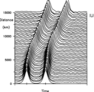
Fig. 1 shows the soliton pair propagating along the fiber with T, = 17.1 ps, La = 30 km,

D

= 2 p s M n m , A D = 0 and 5.9 pulsewidth separation. The total distance shown in Fig. 1 is 15000 km, and the bit rate is 9.91 Gbts/s. One can see that the pulse shapes distort after propagating about 8400 km, and the two solitons collide at about 10500 km. In lossless case, the solitons collide at 5260 km. Fig. 2 shows the condition as in Fig. 1 except that the optical filters with 2.1-nm bandwidth are used after each amplifier. The loss caused by the filter is compensated by the amplifier. We can see that, not only the soliton interaction is reduced, the pulse shapes also maintain well. The filters lead to preferential amplification at the center frequency of the soliton and suppress the nonsoliton component. However, although the pulse shapes maintain well, the pulse separation deviates one-tenth of the original separation after propagating 15000 km. When there exists

(3)

CHI et al.: MAXIMUM BIT RATES OF SOLITON COMMUNICATION SYSTEMS 1123

tu I

15000 Distance (km) IUI lo000 5000 0 0 Time Time

Fig. 1. The eVOhtiOn Of soliton pair without filter for transmission distance Fig. 4. The evolution of soliton pair with dispersion variation as shown in

15 OOO km: D = 2 p s w n m ; La = 30 km, Tw = 17.1 ps, and 5.9 pulsewidth

separation. in Fig. 2.

Fig. 3. The amplitude is given by (4). Other parameters are the same as those

IU

I

lime

Fig. 2.

same as those in Fig. 1.

The evolution of soliton pair with filter. Other parameters are the

(p/lan/nm) (propagating distance)

-0.5

0.5b+-z

1 2 3 4 (periodic amplifier spaang)

Fig. 3. Variation of dispersion D .

dispersion variation along the fiber, the performance of the system degrades. The variation of the dispersion parameter AD is assumed to be periodically varied between -0.5 and 0.5 pslkmlnm with a period of 30 km, which is shown in

tu

I

Time

Fig. 5. The evolution of soliton pair with dispersion variation as shown in Fig. 3. The amplitude is given by (5). Other parameters are the same as those in Fig. 4.

Fig. 3. Fig. 4 shows the same case as in Fig. 2 except with the dispersion variation shown in Fig. 3. It is seen that the pulses are not so stable as in Fig. 2, and the significant nonsoliton waves are radiated out though the filters are used. In the presence of the dispersion variation, the average soliton is no longer the fundamental soliton. To overcome this effect, the amplitude of the soliton is amplified following ( 5 ) so that the average soliton is still the fundamental soliton. Fig. 5 shows the evolution of solitons. To compare with Fig. 4, the pulse shapes maintain better, and the radiations are reduced. The pulse shapes distort after propagating about 9OOO km in Fig. 5; while in Fig. 4, the pulse shapes distort in the very beginning.

(4)

10

2ol

I

,

0.25 20.0

1 e

c 8 A D A t O . b + + ₊ + + I I 0 5Ooo 1 0 b O 1sooO Transmission Distonce(km)

Fig. 6. Maximum bit rate against propagation distance. D = 2 ps/km/nm,

La = 30 km. A with filter and without dispersion variation. 0 with filter and dispersion variation. A is according to (5). @ with filter and dispersion variation. A is according to (4).

*

without filter and dispersion variation.

+

D = 16 ps/km/nm fiber with filter.

*

D = 1 ps/km/nm fiber with filter and dispersion variation. A is according to (5).

201 0 0 0 3 0 +-A A A A 0 A A 0

Fig. 6 shows the maximum bit rate versus transmission distance for D = 2 pskm/nm and La = 30 h. Four conditions are shown: 1) without filter, A D = 0, 2 ) with filter, A D = 0, 3) with filter, A D given by Fig. 3 and soliton amplitude A given by (4), 4) with filter, A D given by Fig. 3 and soliton amplitude A given by (5). To obtain the maximum bit rate for a given distance, the three parameters, the pulsewidth, soliton separation, and filter bandwidth are optimized. Fig. 7 shows the corresponding optimal pulsewidth used in Fig. 6. For shorter transmission distance, the maximum bit rate is higher, and the pulsewidth is shorter. In Fig. 7, the ratio L a / z , is also shown. For shorter distance, the ratio is rather high, and the soliton is essentially unstable, and more nonsoliton waves tend to radiate out. Therefore, we use stronger filtering not only to reduce the soliton interaction, but also to filter out the nonsoliton waves. It is noticed that too strong a filtering also distorts the pulse shape. The corresponding optimized filter bandwidth for a given transmission distance is shown in Fig. 8. From Fig. 6, we can see that, without the filter, the maximum

0 0

0.0

I

I 1

0 5000 1

odoo

15000

Transmission Distance(km)

Optimal filter bandwidth of parameter B corresponding to Fig. 6.

Fig. 8.

h P

251

5 , I

0

sob0

loo00

1 5 d O O

Fig. 9. Transmission bit rate versus distance for L , = 30, 40, and 50 km

in D = 1 ps/km/nm fiber with dispersion variation AD = f 0.5 ps/km/nrn. A : amplifier spacing= 30 km. 0: amplifier spacing= 40 km. Ir: amplifier spacing = 50 km.

bit rate is poorest. With the filter, the maximum bit rate is significantly improved, but it decreases in the presence of the dispersion variation if the soliton is not amplified according to (5). When the soliton is amplified according to ( 5 ) , the maximum bit rate is only slightly less than that without the dispersion variations. For 10 O O O - h transmission distance, the maximum bit rate is as high as 10.25 Gbt/s in the presence of the dispersion variation if the soliton is amplified according to (5). In the following, we will consider the maximum bit rate with the filter bandwidth, and the soliton is amplified according to (5) in the presence of the dispersion variation given by Fig. 3.

For the other values of the average dispersion parameter

D , in Fig. 6, the maximum bit rates versus the transmission distance are also shown for comparison. It is seen that, for 1OOOO-h transmission distance, with

D

= 1 ps/km/nm, the maximum bit rate is improved to 13.09 Gbt/s; while with the standard fiber, where D = 16 pskm/nm, the maximum bit rate is reduced to 3.6 Gbt/s. For longer amplifier spacing, the ratio L,/z, increases, and the maximum bit rate decreases. With

D = 1 p s M n m , the maximum bit rates versus the

transmission distance are shown in Fig. 9 for La = 30, 40, and 50 h . For longer amplifier spacing, the soliton is less

(5)

CHI et al.: MAXIMUM BIT RATES OF SOLITON COMMUNICATION SYSTEMS 1125 h

$

30- Y

.-

v

6

-.I -2 20- c

.-

_n

5

3 -.E

10-

1

01 I

0

sob0

loo00 15dOO

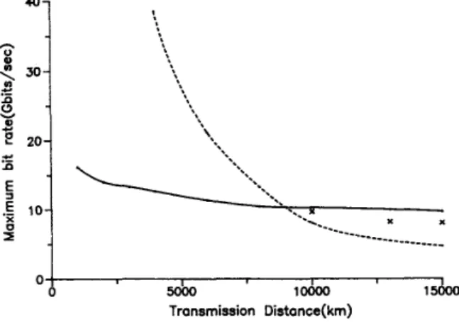
Fig. 10. The bit rate limited by the stability, soliton interaction, and Gor- don-Haus effect for D = 2 ps/km/nm and La = 30 km. - the stability and soliton interaction limit. . . .

. . ..

Gordon-Haus limit. x x x x All

limits met by using narrower filters.

7

0 1 I I

0 5OOo. lad00 lso00

Fig. 11. The bit rate limited by the stability, soliton interaction, and Gor-

don-Haus effect for D = 2 ps/km/nm and La = 50 km.

-

the stability and soliton interaction limit.

. . .

. . .. Gordon-Haus limit. X x x x All

limits met by using narrower filters.

stable, and the maximum bit rate is reduced. However, with 50-km amplifier spacing, the maximum bit rate is still rather high and is 9.9 Gbt/s for 10000-km transmission distance.

decreasing the filter bandwidth to make the limits imposed by the stability, the soliton interaction and Gordon-Haus effect meet simultaneously, and the maximum bit rates are shown in Fig. 10 by the cross symbols. It is seen that the maximum bit rates are only slightly lower than those only limited by the stability and soliton interaction because the timing jitter caused by the Gordon-Haus effect is proportional to the filter IV. COMPARISON OF MAXIMUM BIT RATE LIMITED

BY STABILITY ANDSOLITON bTlERACTION AND

THAT LIMITED BY GORDON-HAUS EFFECT

The Gordon-Haus effect can be overcome by using the optical filter and synchronous modulation. As the optical filter is easier to implement and is suitable for wavelength-division- multiplexing, it is considered in this section. It is known that the Gordon-Haus effect is reduced by decreasing the filter bandwidth [13], [14]. However, as is shown in the previous section, there exists an optimal filter bandwidth to suppress the soliton interaction and filter the radiation waves. Too narrow a bandwidth may distort the pulse shapes. For comparison, the filter bandwidth used to reduce the Gordon-Haus effect is the same as the optimal bandwidth used in the last section.

For the system with 2-ps/km/nm-dispersion parameter, 30-km amplifier spacing, and 10-g-bit error rate, the maximum bit rate for a given transmission distance is shown in Fig. 10 by the dashed line. In Fig. 10, the filter bandwidths are used to overcome the Gordon-Haus effect. The amplifier is assumed to be ideal, and its spontaneous emission factor is unity [18]. The maximum bit rate limited by the stability and soliton interaction is also shown in the figure by the solid line for comparison. We can see that, when the distance is short, the limitation imposed by the stability and soliton interaction is more serious. For the transmission distance longer than 8500 km, the Gordon-Haus effect is more serious. In such a case, the filter bandwidth required to maintain the pulse shapes and pulse separation is not narrow enough to overcome the

bandwidth by a power of four [14], and the slight decrease of the filter bandwidth significantly improves the maximum bit rate. For the maximum bit rate limited by the stability, soliton interaction, and Gordon-Haus effect, it is 16.2 Gbts/s for 1000-km transmission distance and decreases to 8 Gbits/s for 15 000-km transmission distance.

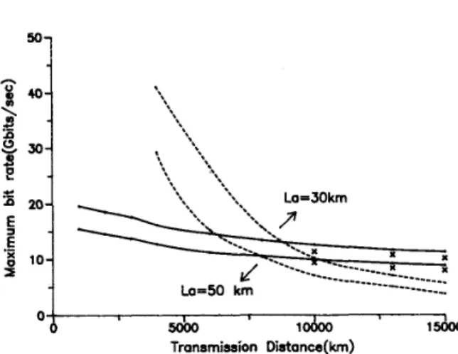
For longer amplifier spacing, the Gordon-Haus effect increases because of higher noise power, and the solitons become more unstable because of higher L a / z o ratio. Therefore, the maximum bit rate decreases as the amplifier spacing increases. Fig. 11 shows the cases with 50-km amplifier spacing, where the meanings of the lines and cross symbols are the same as in Fig. 10. From Fig. 11, the maximum bit rate limited by the stability, soliton interaction, and Gordon-Haus effect is 11.9 Gbt/s for 1000-km transmission distance and also decreases to 5.6 Gbt/s for 15000 -km transmission distance. In the same way, when we consider the system with

D

= 1 ps/km/nm, as shown in Fig. 12, we find that the maximum bit rate limited by the stability, soliton interaction, and Gordon- Haus effect, for La =30 km, is 19.7 Gbt/s at 1000-km transmission distance and decreases to 10 Gbt/s at 15OOO-km transmission distance. Fig. 12 also shows the case for La = 50 km, the maximum bit rate is 15.5 Gbt/s at 1000-km transmission distance and decreases to 7.95 Gbt/s at 15 000-km transmission distance.

Gordon-Haus effect. Further decreasing the filter bandwidth increases the maximum bit rate limited by the Gordon-Haus effect, but decreases the maximum bit rate limited by the stability and soliton interaction. Therefore, the real maximum bit rate lies in the region between the two maxima. If we readjust the parameters by increasing the pulsewidth and

V. CONCLUSION

The maximum bit rate of the soliton communication system with lumped EDFA’s to compensate for the fiber loss and optical filters to reduce the soliton interaction, to filter the radiation waves, and to overcome the Gordon-Haus effect

(6)

0 ‘

sdoo

lOdO0 1&

Transmission Diatance(km)

Fig. 12. The bit rate limited by the stability, soliton interaction, and Gor- don-Haus effect for D = 1 ps/km/nm and La = 30.50 km.

-

the stability and soliton interaction limit .

. . .

. .. Gordon-Haus limit. x x x x All limits met by using narrower filters.

is considered. When the dispersion of the fiber varies from amplifier spacing to amplifier spacing, the maximum bit rate is significantly reduced because the ratio L,/z, is rather high. To overcome the effect, the amplitude of the soliton is amplified so that it is still the average soliton corresponding to the fiber dispersion for an amplifier spacing. Thus, the maximum bit rate is only slightly less than that without dispersion variations. For a given distance, the maximum bit rates considering the stability and soliton interaction are obtained for several dispersion parameters and amplifier spacing. The results are compared with those limited by the Gordon-Haus effect. For shorter transmission distance, the maximum bit rate is limited by the stability and soliton interaction. For longer transmission distance, the maximum bit rate is limited by the Gordon-Haus effect.

111

121 r31

wo1.

M. Nakazawa, Y. Kimura, K. Suzuki, and H. Kubota, “Wavelength multiple soliton amplification and transmission with an E$+-doped optical fiber,” J. Appl. Phys., vol. 66, pp. 2803-2812, 1989.

L. F. Mollenauer, M. J. Neubelt, S. G. Evangelides, J. P. Gordon, J. R. Simpson, and L. G. Cohen, “Experimental study of soliton transmission over more than 10000 km in dispersion-shifted fiber,” Opt. Len., vol.

L. F. Mollenauer, E. Lichtman, G. T. Harvey, M. J. Neubelt, and B. M. Nyman, “Demonstration of error-free soliton transmission over more than 15000 km at 5 Gbit/s, single-channel, and over more than 11 000

km at 10 Gbit/s in two-channel WDM,” Electron. Lett., vol. 28, pp. 192-794, 1992.

A. Hasegawa and Y. Kodama, “Guiding-center soliton in optical fibers,”

Opt. Lett., vol. 15, pp. 1443-1445, 1990.

L. F. Mollenauer, S. G. Evangelides, and H. A. Haus, “Long-distance soliton propagation using lumped amplifiers and dispersion shifted fiber,” J. Lightwave Technol., vol. 9, pp. 194-196, 1991.

K. J. Blow and N. J. Doran, “Average soliton dynamics and the operation of soliton systems with lumued amplifiers,” ZEEE Photon. Technol. Lett..

15, pp. 1203-1205, 1990.

-

-vol. 3, pp.-369-371, 1991:

J. P. Gordon and H. A. Haus, “Random walk of coherently amplified solitons in optical fiber transmission,” Opt. Lett., vol. 11, pp. 665-667, 1986.

Y. Kodama and S. Wabnitz, “Reduction of soliton interaction forces by bandwidth limited amplification,” Electron. Lett., vol. 27, pp.

1931-1933, 1991.

A. Mecozzi, J. D. Moores, H. A. Haus, and Y. Lai, “Soliton transmission control,” Opt. Lett., vol. 16, pp. 1841-1843, 1991.

A. Mecozzi et al., “Modulation and filtering control of soliton transmis- sion,” J. Opt. Soc. Am. E , vol. 9, pp. 1350-1357, 1992.

M. Nakazawa et al., “10 Gbit/s soliton data transmission over one million kilometres,” Electron. Len., vol. 27, pp. 1270-1272, 1991. M. Nakazawa et al., “Infinite-distance soliton transmission with soliton controls in time and frequency domains,” Electron. Lett., vol. 28, pp. 1099-1100, 1992.

H. Kubota and M. Nakazawa, “Soliton transmission control in time and frequency domains,”ZEEE J. Quantum Electron., vol. 29, pp. 2189-2197, 1993.

D. Marcuse, “An alternative derivation of the Gordon-Haus effect,” J.

Lighiwuve Technol., vol. 10, pp. 273-278, 1992.

Sien Chi, photograph and biography not available at the time of publication.

REFERENCES

A. Hasegawa and F. D. Tappert, “Transmission of stationary nonlinear optical pulses in dispersive dielectric fibers 1. Anomalous dispersion,”

Appl. Phys. Len., vol. 23, pp. 142-144, 1973.

A. Hasegawa, “Amplification and reshaping of optical solitons in glass fiber-IV,” Opt. Lett., vol. 8, pp. 650-652, 1983.

-, “Numerical study of optical soliton transmission amplified periodically by the stimulated Raman process,” Appl. Opt., vol. 23, pp. 3302-3309, 1984.

Jeng-Cherng Dung, photograph and biography not available at the time of

publication.

Senfar Wen, photograph and biography not available at the time of publication.