Practical Papercraft Models from Meshes

(1)

Practical Papercraft Models from Meshes

Student: Ying-Tsung Li

Advisor: Dr. Jung-Hong Chuang

Dr. Wen-Chieh Lin

Institute of Computer Science and Engineering

College of Computer Science

National Chiao Tung University

ABSTRACT

We present a new approach to generate papercraft models from meshes. The input mesh is ap-proximated by a set of quadric surface proxies. Each quadric proxy is then cut and unfolded into a 2D papercraft pattern. Our method has the following advantages : First, we produce smoother papercraft models than previous methods. Second, the 2D patterns of papercraft models are easy to cut and glue. Finally, the 2D patterns of papercraft models are more meaningful due to the pre-defined cutting rules. We demonstrate this by physically assembling papercraft models from our algorithm.

(2)

Acknowledgments

I would like to thank my advisors, Professor Jung-Hong Chuang, and Wen-Chieh Lin for their guidance, inspirations, and encouragement. I also want to thank another faculty, Sai-Keung Wong. He give me many useful suggestions. I am grateful to Tan-Chi Ho for his comments and advices. Thanks to my colleagues in CGGM lab.: Chin-Hsian Chang, Kuang-Wei Fu, Hsin-Hsiao Lin, Yueh-Tse Chen, Ta-En Chen, Hong-Xuan Ji, Cheng-Min Liu, Jau-An Yang, Tsung-Shian Huang, and Chien-Kai Lo for their assistances and discussions. It is pleasure to be with all of you in the pass two years. Lastly, I would like to thank my parents for their love, and support.

(3)

List of Figures

1.1 Papercraft models. . . 2 1.2 Model with pre-defined cutting rules and its unfolded 2D pattern. . . 3 3.1 System flow of our papercrafting algorithm. . . 10 3.2 Triangle to triangle distance : a,c are the center respect to triangle tiand triangle

tj, and b is the middle of the shared edge between tj and tj. Dij = |ab| + |bc|. . 14

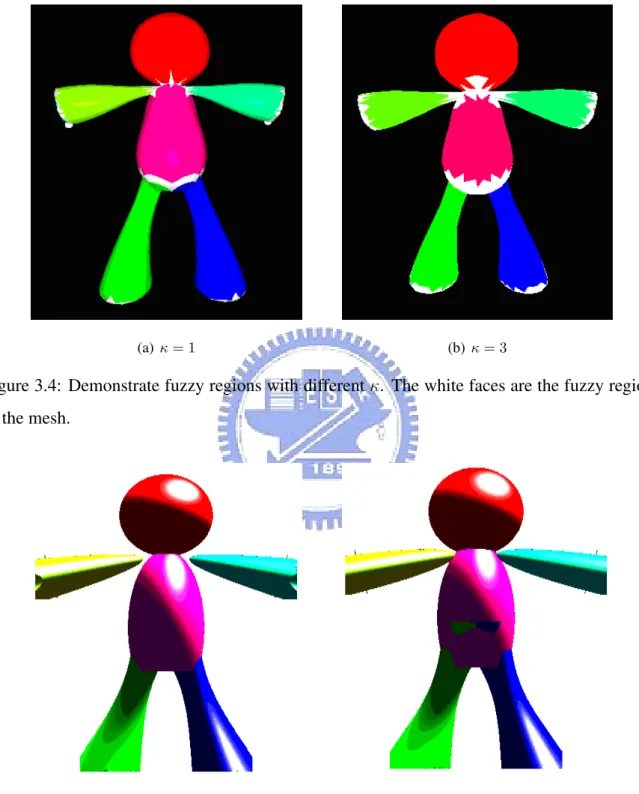
3.3 Example that is used to illustrate the effect of fuzzy segment. . . 16 3.4 Demonstrate fuzzy regions with different κ. The white faces are the fuzzy

re-gions of the mesh. . . 17 3.5 The fuzzy segmentation results with different κ. . . 17 3.6 Three quadric surfaces and their intersection curves. The blue lines are the

intersection curve. . . 18 3.7 An example to illustrate Algo.3.1. . . 19 3.8 The tangent direction of the intersection curve at p is Ni(p) × Nj(p) which is

perpendicular out the paper. . . 21 3.9 Cutting rule for ellipsoid type and the example quadric that apply the rule. . . . 29 3.10 A example of vertical cut line that preserve 10 percent length between every

two intersection points. . . 29 3.11 The cutting rule for hyperboloid one sheet, hyperboloid two sheets, elliptic

paraboloid and hyperboloid paraboloid types. . . 30

(6)

3.12 Example of cutting hyperbolic paraboloid surface. . . 30

3.13 Parametrize the model in 3.9(b) with different parametrization methods . . . . 32

4.1 The problem on the bottom of the body in ”small people” model. . . 35

4.2 The different between body and legs in original model and approximated model. 36 4.3 Quadric surface fitting result that the arms are disconnect to body. . . 36

4.4 The small people model. . . 37

4.5 The chess model. . . 38

5.1 The comparison of previous work [18] [20] [17] with our results. . . 40

(7)

List of Tables

3.1 Three nonzero eigenvalues . . . 24

3.2 Two nonzero eigenvalues . . . 25

3.3 One nonzero eigenvalue . . . 25

3.4 Zero nonzero eigenvalue . . . 26

3.5 Quadric type and the corresponding parametric function, where v = [x, y, z] is a point on the quadric surface. . . 27

3.6 Quadric type and the corresponding inverse parametric function, where p = [u, v] is a point on the parametric space. . . 33

(8)

C H A P T E R

1

Introduction

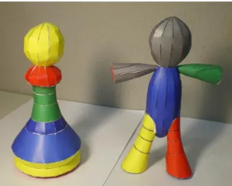
Papercraft models are models that are assembled from a set of 2D patterns on the paper (Fig.1.1). The paper layout is usually generated by hand or interactively by various companies. This task is difficult for a normal user and we want to perform this automatically. There are two challenges to generate papercraft models automatically and practically. The first challenge is to segment a given model into parts that fit human’s expectation and add cutting lines on each part to increase the developability. A meaningful part is always not a developable surface, so we need to apply cutting on it to increase the developability of this part and reduce the stretching when we unfold this patch. The second challenge is to unfold parts meaningfully. Some automatically cutting algorithm, like [14], will add the cut lines at the position that has the highest distortion. The cutting lines generated by those algorithm are irregular and are not easy to cut and glue. We want to cut patches meaningfully because the 2D patterns of man made papercraft model always follow some kinds of cutting rules.

To address the first issue, we use the quadric surface as the basic fitting primitive rather than simple developable surface like [20] [17]. Because quadric surfaces are more complex than developable surfaces, using quadric surface as the basic primitive can reduce the number of patches to approximate the input mesh. Thus, the assembled models which are fitted by quadric

(9)

1.1 Contribution 2

Figure 1.1: Papercraft models.

surfaces are smoother than models fitted by developable patches because the crease lines will appear on the patches boundary. For example, an ellipsoid can be consider as a single patch when quadric surfaces are the basic fitting primitives but it will have several patches when it is fitted by developable surfaces and it will not smooth between the patch boundary due to lack of G1 _continuity.

For the second issue, we cut the quadric surfaces using pre-defined cutting rules rather than automatically cutting algorithm like [14]. With pre-defined cutting rules, the unfolded 2D pattern will have the following advantages :

• User can figure out the assembled shape of the unfolded 2D pattern (Fig.1.2). • The unfolded 2D pattern’s boundary is smooth and is easy to cut and glue.

1.1 Contribution

The contributions of this thesis can be summarized as:

(10)

1.2 Outline 3

(a) Half of an ellipsoid type model with the yel-low lines as the cut lines.

(b) The unfolded 2D pattern of the half ellip-soid.

Figure 1.2: Model with pre-defined cutting rules and its unfolded 2D pattern. • The boundary of unfolded 2D pattern are smooth and it is easy to cut and glue. • The 2D pattern is correspond to a meaningful part of original 3D model.

• The 2D pattern’s shape is meaningful that user can predict the assembled shape in 3D. • The assembled papercraft model is smoother than previous paper because of using quadric

surfaces as the basic fitting primitive rather than using simple developable surfaces.

1.2 Outline

The rest of the thesis is organized as follows: Chapter 2 gives the literature review, the back-ground of mesh segmentation, shape approximation and related system for automatically gen-erating papercraft models. Chapter 3 illustrate our proposed algorithm to generate a papercraft model from an input mesh. Chapter 4 shows our results from our approach. In the end, conclu-sions and future work are discussed in Chapter 5.

(11)

C H A P T E R

2

Related work

The system we present shares common goals with a number of previously papers. Therefor, we introduce some related research.

2.1 Variational Shape Approximation

Cohen-Steiner et. al [6] propose a shape approximation algorithm based on clustering approach to optimally approximate a mesh surface by a specified number of planar faces. This optimiza-tion problem is solved as a discrete partioptimiza-tion problem using the Lloyd algorithm [16], which is commonly used for solving the k-mean problem in data clustering. There are two iterative steps in this method: mesh partition and fitting a plane face, called a proxy, to each partitioned region. This method proves effective especially for extracting features and planar regions, but tends to produce an overly large number of planar proxies for a good approximation of a freeform sur-face. Because of its optimization nature, the method is often referred to as a variational method. Because this method only extracts the planar regions, the approximated models are piecewise linear in each patches. It does not fit our goal of generating a smooth papercraft models from

(12)

2.1 Variational Shape Approximation 5

meshes.

Wu and Kobbelt [27] extend the work in [6] by introducing spheres, cylinders and rolling ball patches as additional basic proxy types, so that a complex shape can be approximated to the same accuracy by a much fewer number of proxies, leading to a more compact representation. However, these newly added surface types mentioned are still rather restricted, even for CAD models and other man-made objects.

Simari et al. [24] use ellipsoids as the only type of proxies for approximating mesh surfaces, again using the Lloyd method with the error metric being a combination of Euclidean distance, angular distance and curvature distance. The segmentation boundaries are smoothed by a con-strained relaxation of the boundary vertices.They also approximate the volume bounded by a mesh surface using a union of ellipsoids, where whole ellipsoids, rather than ellipsoidal surface patches, are used. This method is useful for collision detection but not useful for the purpose of papercrafting because the papercraft models do not consider the volume informations inside its surface.

Attene et al. [2] use hierarchical face clustering algorithm to approximate triangle meshes into a set of primitives include which planes, spheres and cylinders. This method can generate a binary tree of clusters which is fitted by one of the primitives in the bottom up scheme. The disadvantage of this method is that we can not get desire number of segment directly, we need to construct the binary tree first to eliminate the number of patches one by one. It takes too much time for processing large models.

Yan et al. [28] use the same framework as [6] [27] [24] but extens the types of proxy into the general quadric surfaces. Yan enhance the algorithm’s performance by using Taubin’s second order approximation to approximate the distance from some point to quadric surface [26]. The region boundaries are smoothed by graph cut method. We modified this method to fit the purpose of papercrafting by constraining some extreme cases that are nearly planar.

(13)

2.2 Paper Crafting 6

2.2 Paper Crafting

Papercraft models are the models which can be assembled from a set of 2D patterns on papers. The work for automatically generating papercraft models from meshes is to approximate the input mesh surface by a set of patches and these patches are unfolded into 2D paper. Because the paper can not stretch, crease and tear, these patches must be developable or nearly developable. There are three types of methods to achieve this goal:

Approximate by developable surfaces Elber [8] proposed a method for approximating NURBs by a set of developable strips. That work treats only a single surface patch, as opposed to mod-els with complex geometry and topology. Elber also uses quite a loose upper bound on the Hausdorff distance as an error approximation. This bound can be far from the true Hausdorff distance, resulting in a much larger number of strips than necessary.

Massarwi et al. [17] approximate input mesh by a set of piecewise-developable surfaces which are generalized cylinder represented as a strip of triangles. They enhance Elber’s method by computing more accurate Hausdorff distance between the input mesh and its piecewise-developable approximation. They also propose a framework to handle more complex meshes.

Shatz et al. [20] use conic surface as proxy surfaces, but additionally consider the error between the triangles and the conic surface. The proxy conic surfaces are treated as the final approximation surfaces and can be directly unfolded. Because of the error between the proxy conic and the origin meshes, sometimes the boundaries between the neighboring conic surfaces will be unstable and must be specially dealt with. They only apply additional optimization pro-cess on suce unstable boundaries, so seams will probably appear between neighboring conics.

Approximate by triangle strips Mitani and Suzuki [18] propose a algorithm that first seg-ment the meshes into parts based on features. Then these parts are approximated with triangle strips. The same process repeat until all triangles are covered by some triangle strips. The tri-angle generated from their algorithm tend to have long boundaries which are not convenient for

(14)

2.3 Mesh Parameterization 7

gluing. Another problem is that the method does not consider any error metric, the only way to control the error is the predefined width of the triangle strips, which is not flexible.

Approximate by nearly developable patches Julius et al. [11] propose using developability as error metric to segment the meshes. Their algorithm is based on region growing framework and use a Lloyd scheme. For each patch, a conic is used as a proxy surface. Because the angle between the conic’s axis and normal on the surface is constant, the developable error metris is defined as

(NC· · · nt− cos θC)2,

where NC is the axis of the conic, nt is the normal of the triangle, θ is the constant angle.

They additionally consider the compactness and boundary smoothness of the patch as error metrics and use the product of the three weighted error metrics as the region growing error metric. At each iteration, faces with the smallest error are inserted into the patches until all faces are covered, then the optimized proxy conics are computed to fit the patches, the process repeat until converge. Because the algorithm only segment the mesh, a parametrization method mustbe used to unfold patches into a plane. Because there are no isometric parametrization for general patches, distortion will still be introduced in the process.

2.3 Mesh Parameterization

Mesh parameterization is to find a parametric function that map the mesh surface onto the 2D parametric domain. There are two goals for mesh parameterization to achieve. The first one is to preserve area between 2D surface and the 3D surface. The second one is to preserve angle and is called conformal parametrization. The boundary type of the 2D surface also have two types : the restrict type and the free type. The restrict type sometimes use square as the boundary of 2D domain and solve the convex combination problem to get the parametric function [10] [9]. The free type will first fix some verties as the anchors and reconstruct the parametric function with the angle constrains [14] [21]. For the purpose of papercrafting, we need a conformal

(15)

2.3 Mesh Parameterization 8

parametrization that also preserve the edge length between 3D and 2D. Following are the papers that are conformal parametrization.

Sheffer et al. [21] presented Angle-Based Flattening (ABF) method that defined an angle preservation metric by which the parameterization was computed in the angle space and then converted into a 2D coordinate. When converting the parameterization from the angle space into planar coordinates, natural boundaries were automatically formed. Sheffer et al. [22] presented ABF++ method that enhance the performance of ABF method based on numerical methods (se-quential linear quadratic programming) and algebraic transforms of the initial problem. These transforms were combined with a multigrid optimization framework to further improve perfor-mances. Zayer et al. [29] use a linear approximate of the initial ABF equations. The time-space complexity and accuracy of the solution are to a great extent affected by the kind of approxima-tion used. They reformulate the problem based on the noapproxima-tion of error of estimaapproxima-tion. The error induced by this linearization is quadratic in terms of the error in angles and the validity of the approximation is further supported by numerical results.

Levy et al. [14] and Desbrun et al. [7] are parameterizations that also give free boundaries. It is difficult to add special constraints about the shearing (for shape) or stretching (for length) on boundaries in their linear systems. However, the positions of boundary vertices are more important than interior vertices since the shape and the area of a planar domain are essentially defined by the boundary vertices.

(16)

C H A P T E R

3

Algorithm

This chapter describes algorithm of making papercraft models from meshes. We first give an overview of our proposed method (Subsection 3.1). Next, we describe the detail of each step of the algorithm, including Mesh Segmentation (Subsection 3.2), Fuzzy Segmentation (Sub-section 3.3), Boundary Extraction (Sub(Sub-section 3.4), Parametrization and Apply Cutting Rules (Subsection 3.5) and finally Unfold Quadric Patches (Subsection 3.6).

3.1 Overview

The aim of the algorithm is to segment the input mesh into a set of parts which includes several segments that can be well approximated by quadric surfaces and planes. Each part can be unfolded into 2D patterns which are meaningful and can be easily cut and glued. In order to achieve this goal, we do the following processes to our input meshes. First, we may segment the input mesh into parts manually or by some part-based segmentation algorithm and adapt quadric surface extraction method which is proposed by Yan et. al.[28] for further segmenting parts into quadric surface patches. Then, we use the idea of fuzzy region to avoid generating quadric

(17)

3.1 Overview 10

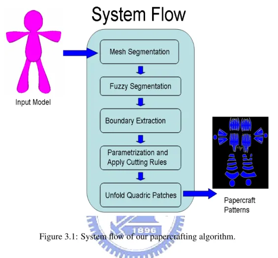
Figure 3.1: System flow of our papercrafting algorithm.

surface patches which have no intersection with others. The third step is to find the intersection curves between these quadric surfaces. In this step, we must avoid not to find curves which are not really needed for our algorithm by using the concept of Object-Oriented Bounding Box of the quadric surface. Next, we transform each quadric surface into its local parametric space and apply appropriate cutting rules on the parametric domain. For minimizing the number of quadric surface patches, we provide a function that is used to rotate the local parametric space to avoid some awful cutting results. Then, we triangulate each quadric patch on the parametric domain and restore from 2D to 3D by apply each patch’s inverse parametrization. Finally, we use several conformal parametrization methods to unfold each quadric patch and use a metric to choose the best parametrization result as our final unfold 2D pattern. Fig.3.1 is the system flow of our algorithm.

(18)

3.2 Mesh Segmentation 11

3.2 Mesh Segmentation

In order to segment input meshes into a set of meaningful quadric patches, we do the following two steps : pre-segmentation and quadric surface extraction. The pre-segmentation step is optional and can be done manually or by some part-based segmentation algorithms like [12] [13] [5] [15]. The quadric surface extraction is based on Yan et. at.[28] and is modified to fit the purpose for papercrafting. We will introduce the variational framework first and demonstrate the error metric and fitting scheme that Yan used for quadric surfaces extraction. Then we will do some modifications to fit the purpose of papercrafting.

3.2.1 Variational Framework

Let M denote an input mesh surface, and T denote the set of triangles of M. Suppose that M is partitioned into n non-overlapping regions, denoted as R = {Ri}ni =1, each region Ri

containing a set of triangle Ti = {tki} ni

k =1 such ∪ni =1Ti = T . Each region Ri is approximated

by a quadric proxy Pi (including the plane as a special case). A seed face Si of Pi is the

smallest error face in Ti. In a variational framework the optimal partition R = {Ri}ni =1 is

found by minimizing the following objective function : E(R, P) = n X i =1 E0(Ri, Pi) = n X i =1 ni X k =1 d(t_ki, Pi) (3.1)

where d(t_ki, Pi) measure the error between the triangle tkiand the proxy Pi. Therefore, E0(Ri, Pi)

is the error between the region Ri and its approximating proxy Pi. Lloyd’s algorithm minimizes

Eq.3.1 through iterative partition and fitting.

3.2.1.1 Error Metric for Proxies

In order to use quadric surface as the fitting proxy, they have to define the error metric quadric proxies. The error metric for quadric proxies extraction is defined as the L2 _distance.

(19)

use Taubin’s second order approximation of the Euclidean δd(p, Z(f )) [26] from point p to the

quadric surface Z(f ) as the approximate distance. Based on this distance, the approximated L2 distance for a triangle t to quadric surface Piis defined as :

d(t, Pi) = 1 m m X k=1 δd(pk, Zi(f ))2· · · A

where {pk}mk=1 are uniformly sampled points on the triangle t and A is the area of t which

is a weighting factor to account for triangles of different size. The approximated L2 distance between Riand Pi is then defined as:

E0(Ri, Pi) = X tj∈Ri d(tj, Pi)/ X tj∈Ri Aj.

To have a uniform comparison, all mesh are scaled uniformly to fit in a rectangular box with the diagonal length being 1.

3.2.1.2 Quadric Surface fitting

Given a region Ri, we need to fit a quadric surface to Riin L2metric. For performance concern,

they use Taubin’s method [25] based on a first-order approximation of L2 _{metric for quadric}

surface fitting.

Let f (x, y, z) = 0 be a quadric surface. The squared distance from a point p to the im-plicit surface Z(f ) = {(x, y, z)|f (x, y, z) = 0, x, y, z ∈ R} is approximated as d(p, Z(f ))2 ≈

f (p)2

k5f (p)k2. The sum of approximated squared distance is following [28]

1 A ni X k=1 Z tk d(p, Z(f ))2dp ≈ 1 A Pni k=1 R tkf (p) 2_dp 1 A Pni k=1 R tkk∇f (p)k 2_dp = st_M ts st_N ts , (3.2)

where M , N are coefficient metrics and s =< C0, C1, ..., C9 >T and A is the sum of the areas

of all triangles in Ri. The fitting problem is reduced to computing the eigenvector of M − λNt

(20)

3.2.2 Modification for Papercrafting

By using Yan’s method, we find that plane proxy is rarely happened due to small noises of mesh data. Mostly near planar regions are fitted as the quadric type of hyperboloid of two sheets which has small coefficients and is fitted to some region in the quadric proxy which is far from proxy’s center. For papercrafting, we prefer to choose plane proxy than hyperboloid of two sheets proxy in such a region. In order to achieve this goal, we fit each region Ri as quadric

proxy Pi and plane proxy Pi0 at the same time. The fitting error is denote as Ei and Ei0. If Ei0

is smaller than Ei or Ei0 is larger than Ei but is smaller than user defined plane tolerance δplane,

we choose P_i0 as Ri’s approximating proxy. Otherwise we choose Pi as Ri’s approximating

(21)

3.3 Fuzzy Segmentation 14

3.3 Fuzzy Segmentation

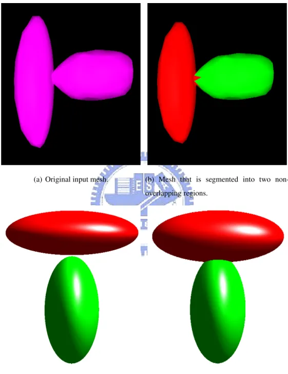
There are some problems in the original quadric surface extraction method [28]. For exam-ple, the input mesh Fig.3.3(a) is compose of two ellipsoids like object. When we apply mesh segmentation, we can segment this mesh into two regions which have the quadric proxies of ellipsoid type Fig.3.3(b). Fig.3.3(c) is the quadric surface of these two quadric proxies which are drawn by MATLAB. From Fig.3.3(c), we can see that the two quadric surfaces are dis-connected. This is a crucial problem for papercrafting and we want solve this problem by automatically connect these two quadric surface. We find out that this problem is due to lack of informations of triangles which are near the region boundary during the process of quadric surface fitting. When we apply quadric surface fitting, we only consider the triangles in Ri.

Triangles which are near the ∂Ri and not belong to Ri also have useful information for fitting

process because these triangles also have low error respect to Ri. Therefore, we define a fuzzy

region F Ri which includes triangles nearby the region boundary for each region Ri. Before

we give the definition of F Ri, we first define the triangle to triangle distance Dij as follow

(Fig.3.2):

Dij =

undef ined , tiis not adjacency totj

ab + cb , tiis adjacency totj

, where a, c are the center respect to triangle tiand tj and b is the middle of the shared edge of

tiand tj. Then, we define σ as the average triangle to triangle distance of whole mesh.

Figure 3.2: Triangle to triangle distance : a,c are the center respect to triangle ti and triangle tj,

(22)

The fuzzy region F Ri is defined as :

F Ri = {t|∀t ∈ T , t 6∈ Riand the distance of t to ∂Riis less than κσ},

where κ is the user defined parameter that can control the size of fuzzy region. Now, we adapt the original fitting method by adding weighting for each triangle and incorporating triangles in fuzzy region. The original quadric surface fitting equation 3.2 is modified as follow:

1 A ni X k=1 wi Z tk d(p, Z(f ))2dp ≈ 1 A Pni k=1wi R tkf (p) 2_dp 1 A Pni k=1wiRtkk∇f (p)k 2_dp = st_M ts st_N ts ,

where Mt, Ntare coefficient matrices, niis the number of triangles of |Ri∪ F Ri|, A is the sum

of the areas of all triangles in Ri∪ F Ri, and wi is the additional weighting for each triangle in

Ri ∪ F Ri. The weighting wifor each triangle tiis defined as :

wi = {

1.0 , ti ∈ Ri

1.5 × (0.5)bdist(ti,∂Ri)σ c , t_i ∈ F R_i

Through the new fitting scheme, the resulting quadric proxies will not be disconnected Fig. 3.3(d). The disadvantage of using fuzzy region is increasing fitting error, because the resulting quadric proxy Pi is not only best fit to the region Ri but also include the nearby region F Ri.

The quadric proxy with fuzzy region looks fatter than the quadric proxy without fuzzy region. Figure3.5 shows the fuzzy regions which are marked as the white faces with different κ value. Figure 3.5 shows the fitting results with different κ values.

(23)

(a) Original input mesh. (b) Mesh that is segmented into two

non-overlapping regions.

(c) Without fuzzy segmentation, quadric prox-ies are disconnected.

(d) With fuzzy segmentation, quadric proxies are connected.

(24)

(a) κ = 1 (b) κ = 3

Figure 3.4: Demonstrate fuzzy regions with different κ. The white faces are the fuzzy regions of the mesh.

(a) With κ = 1, the arm is disconnect to body. (b) With κ = 3, the arm is connect to body but the legs become fatter.

(25)

3.4 Boundary Extraction 18

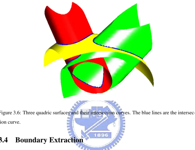
Figure 3.6: Three quadric surfaces and their intersection curves. The blue lines are the intersec-tion curve.

3.4 Boundary Extraction

After the previous steps, the mesh has been segmented into a set of non-overlapping regions. Each region Ri has its own quadric proxy Pi. Define Ni be the set of regions which is

adja-cency to Ri. The problem of finding Pi’s real boundary becomes finding the quadric surface

intersection between Pi to the proxy of every region in Ni (Fig.3.6). Because finding quadric

surface intersection exactly is very hard, we use a marching like method to get an acceptable result. This method has two steps and can apply to two adjacency regions. Firstly, we need to find a starting point that is on the intersection curve of these two quadric surface(Sec.3.4.1). Secondly, we trace from the starting point along the curve’s tangent direction until reaching starting point again (Sec.3.4.2). For convenience, we denote Ri and Rj are the regions which

(26)

3.4.1 Find Starting Point

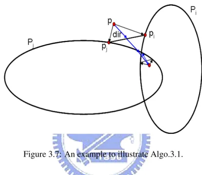
We pick an arbitrary vertex on the boundary as our initial guess point p. Then, we use an iterative algorithm to pull p to the intersection curve (Algo.3.1). The function ”Project” projects a point p onto the quadric surface P. Fig.3.7 is an example of this procedure.

Figure 3.7: An example to illustrate Algo.3.1.

At the end of the find starting point algorithm, we need to check whether the starting point we found is correct or not. A correct starting point means the distance d of of |ppi| + |ppj| are

less than some user defined threshold. One of the incorrect case may occur when the starting point reaches a position that is nearly collinear to the two projected points piand pj. In this case,

the starting point may oscillate on the line of pipj and will not come closer to the intersection

curve. In order to avoid this problem, we change the quadric surface Pi to its pencil quadric

Q = Pi + λPj and find the intersection curve between the quadric surface Q and Pj. In our

implementation, λ starts from 1 until we find a correct intersection point.

3.4.2 Tracing Along Tangent Direction

After finding a correct starting point on the intersection curve, we can trace the entire curve along the curve’s tangent direction −→t . Let Gi(x, y, z) = ∇fi(x, y, z) where fi(x, y, z) is the

(27)

Algorithm 3.1: The algorithm of finding first intersection point //step 1: Choose an arbitrary vertex on boundary

p = any vertex ∈ B

//step 2: Iterative optimizes p to the intersection curve for( i = 0 ; i < numiter ; i++ ) {

// Compute the search direction pi = Project(Pi, p)

pj = Project(Pj, p)

dir = p − pi+pj

2

// Walk from p along direction dir until crossing both quadric surface signi = Pi(p) signj = Pj(p) p0 = p do { p0 = p0+ dir sign0_i = Pi(p0) sign0_j = Pj(p0)

}while(signi× sign0i > 0 || signj × sign0j > 0)

p = p0 }

(28)

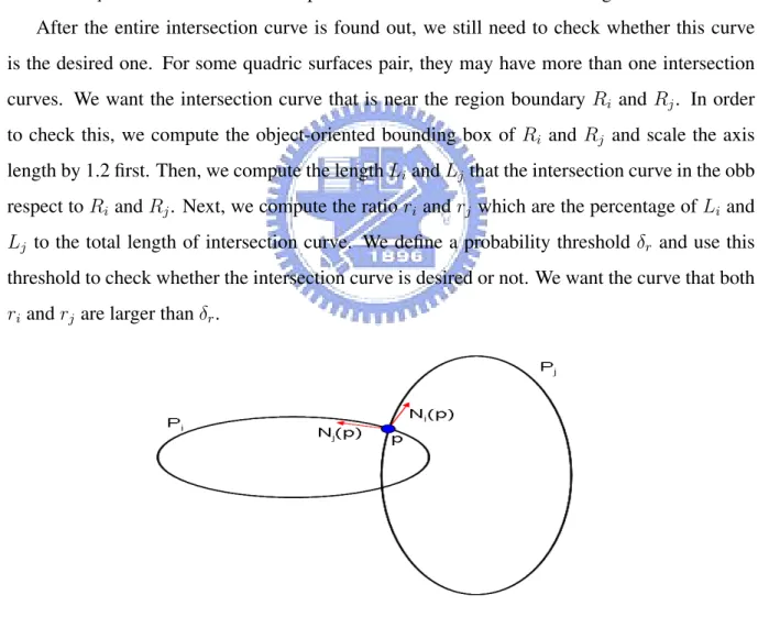
implicit function of quadric surface Pi and Ni(x, y, z) = |GGii(x,y,z)(x,y,z)|. The curve’s tangent

direc-tion−→t at p is derived as Ni(p) × Nj(p) which is perpendicular out of the paper (Fig.3.8). With

the point p and the tangent direction−→t at p, we can shoot from p to next intersection point p0 with constant shooting distance. Due to numerical error of computer program, we must do some correction to p after every shooting step to avoid p go away from real intersection curve too far. This correction is done by projecting p to quadric surfaces Pi and Pj and get two projected

points p1 and p2. Then, we correct p by p = p+p1+p2₃ . The tracing process terminates until the

distance of p and the first intersection point is less than the constant shooting distance.

After the entire intersection curve is found out, we still need to check whether this curve is the desired one. For some quadric surfaces pair, they may have more than one intersection curves. We want the intersection curve that is near the region boundary Ri and Rj. In order

to check this, we compute the object-oriented bounding box of Ri and Rj and scale the axis

length by 1.2 first. Then, we compute the length Liand Lj that the intersection curve in the obb

respect to Ri and Rj. Next, we compute the ratio ri and rj which are the percentage of Li and

Lj to the total length of intersection curve. We define a probability threshold δr and use this

threshold to check whether the intersection curve is desired or not. We want the curve that both ri and rj are larger than δr.

Figure 3.8: The tangent direction of the intersection curve at p is Ni(p) × Nj(p) which is

(29)

3.5 Parametrization and Apply Cutting Rule 22

3.5 Parametrization and Apply Cutting Rule

Because the quadric surface are not all developable, we need to add some cutting lines on the surface to increase the developability. For the purpose of practical papercrafting ,we want the cutting lines are added in some pre-defined rules that fulfill human’s expectation. The cutting rules are defined on the 2D parametric space. In order to apply cutting rules on quadric proxy, we do not add cutting lines on 3D surface directly. We need to transform each proxy into its local parametric space. There are four steps to achieve this goal. First, we need to classify the type of the quadric proxy (Subsection 3.5.1). Next, we transform this quadric proxy to its canonical form and parametrize it by predefined parametric function(Subsection 3.5.2). Finally, we apply cutting rules on the 2D patches (subsection .3.5.3).

3.5.1 Classify quadric type

The quadric surfaces can be defined as the implicit function

f (x) = xTAx + BTx + c = 0 (3.3)

where A is a 3 × 3 nonzero symmetric matrix, B is a 3 × 1 vector, and c is a scalar.

The surface type of each quadric surface can be characterized by analyzing the eigenvalue of matrix A. Since the matrix A is symmetric, it has an eigendecomposition

A = RDRT (3.4)

where R = [v0|v1|v2] is a rotation matrix whose columns vi are linearly independent

eigen-vectors of Ai, and where D = Diag(d0, d1, d2) is a diagonal matrix of eigenvalues of A. The

eigenvector vicorresponds to the eigenvalue di.

Define y = RTx and e = RT_{b. Equation 3.3 may be written as}

(30)

Let y have components labeled yi and let e have components labeled ei for 0 ≤ i ≤ 2. Equation

3.5 becomes

d0y02+ d1y12+ d2y22+ e0y0+ e1y1+ e2y2+ c = 0 (3.6)

If any of the diare not zero, we can complete the square on the diterms:

diyi2+ eiyi = di(yi+ ei 2di )2− e 2 i 4di (3.7) This is the basis for the classification, but requires us to analyze the signs of the di. When a value

di is zero, we will then have to analyze the sign of the corresponding ei value. In preparation

for the classification, define

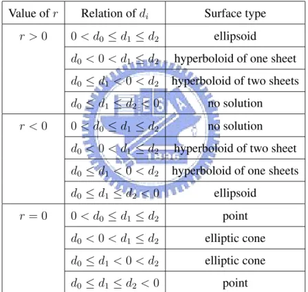
r = −c + 2 X i=0,di6=0 e2 i 4di (3.8) The classifications are depend on the signs of the di, ei, and r. We assume that the eigenvalues

are to be ordered as d0 ≤ d1 ≤ d2so that the classification can be summarized as table 3.1, 3.2,

3.3 and 3.4. For more details, the reader is referred elsewhere Boehm et al.[3] and Schneider et al.[19].

(31)

Table 3.1: Three nonzero eigenvalues

Value of r Relation of di Surface type

r > 0 0 < d0 ≤ d1 ≤ d2 ellipsoid

d0 < 0 < d1 ≤ d2 hyperboloid of one sheet

d0 ≤ d1 < 0 < d2 hyperboloid of two sheets

d0 ≤ d1 ≤ d2 < 0 no solution

r < 0 0 < d0 ≤ d1 ≤ d2 no solution

d0 < 0 < d1 ≤ d2 hyperboloid of two sheet

d0 ≤ d1 < 0 < d2 hyperboloid of one sheets

d0 ≤ d1 ≤ d2 < 0 ellipsoid

r = 0 0 < d0 ≤ d1 ≤ d2 point

d0 < 0 < d1 ≤ d2 elliptic cone

d0 ≤ d1 < 0 < d2 elliptic cone

(32)

Table 3.2: Two nonzero eigenvalues

Relation of di Value of ei Value of r Surface type

d0 = 0 < d1 ≤ d2 e0 6= 0 elliptic paraboloid e0 = 0 r > 0 elliptic cylinder r = 0 line r < 0 no solution d0 < 0 = d1 < d2 e1 6= 0 hyperbolic paraboloid e1 = 0 r 6= 0 hyperbolic paraboloid r = 0 two planes d0 ≤ d1 < d2 = 0 e2 6= 0 elliptic paraboloid e2 = 0 r > 0 no solution r = 0 line r < 0 elliptic cylinder

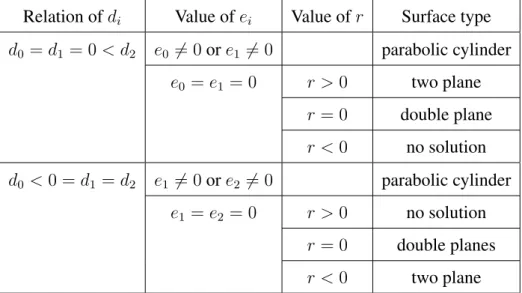
Table 3.3: One nonzero eigenvalue

Relation of di Value of ei Value of r Surface type

d0 = d1 = 0 < d2 e0 6= 0 or e1 6= 0 parabolic cylinder e0 = e1 = 0 r > 0 two plane r = 0 double plane r < 0 no solution d0 < 0 = d1 = d2 e1 6= 0 or e2 6= 0 parabolic cylinder e1 = e2 = 0 r > 0 no solution r = 0 double planes r < 0 two plane

(33)

Table 3.4: Zero nonzero eigenvalue

Value of ei Surface type

e0 6= 0 or e1 6= 0 or e2 6= 0 plane

e0 = e1 = e2 = 0 no solution

3.5.2 Transform to canonical form

In order to transform quadric proxy into canonical form, we use R as the rotation matrix that can transform original quadric proxy to axis-aligned proxy. By equation 3.7, we can get a translation vector T = [T0, T1, T2], Ti = −_2dei

i which can move each axis-aligned quadric proxy’s center

to origin.The detailed method is referred [4]. After we transform each quadric proxy to its canonical form, we can use the predefined parametric function to parametrize it. We choose the parametric function according to its quadric type. The quadric types and the corresponding parametric functions are in the table 3.5.2.

(34)

Quadric Type Parametric function

Parabolic Cylinder u =

z e2

v = y

Elliptic Cylinder u = tan

−1₍y×d0

x×d1)

v = z

Hyperbolic Cylinder u = cos

−1₍y×d0

x×d1)

v = z Elliptic Paraboloid u = tan

−1₍y×d0

x×d1)

v = _ez

2

Hyperbolic Paraboloid u = cos

−1₍y×d0

x×d1)

v = _ez

2

Elliptic Cone u = tan

−1₍d0×y

d1×x)

v = _dz

2

Hyperboloid One Sheet u = tan

−1₍y×d0

x×d1)

v = tan−1(z d2)

Hyperboloid Two Sheets u = sin

−1 (y×d0 x×d1) v = tan−1(_dz 2) Ellipsoid u = tan −1₍y×d0 x×d1) v = sin−1(_dz 2) Plane u = x v = y

Table 3.5: Quadric type and the corresponding parametric function, where v = [x, y, z] is a point on the quadric surface.

(35)

3.5.3 Apply cutting rules

Once we parametrize each quadric proxy into its local parametric space. We add cut lines on the 2D parametric space according to its quadric type. There are three category of quadric surfaces.

Developable quadric This category includes plane, elliptic cylinder, parabolic cylinder, hy-perbolic cylinder and elliptic cone. For this type of quadric, we do not apply any cutting on the 2D pattern.

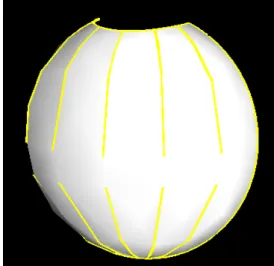
Ellipsoid We use cut lines that cut this ellipsoid like we peel the banana (Fig.3.9(b)). The cutlines are added vertically for every 30 degrees which is starts from -180 to 180 (3.9(a)). For each vertical cut line, we analyze the intersections between this line and the curves on the 2D parametric space. We keep the 10 percents of length between every two adjacency intersection points to avoid small pieces (Fig.3.10).

Others For quadric types of hyperboloid one sheet, hyperboloid two sheets, elliptic paraboloid and hyperboloid paraboloid, we add horizontal cut lines from the bottom to top and all cut lines are evenly spacing on the v-axis (Fig.3.11). We define a minimum vertical spacing δvs to

con-trol the number of horizontal cut lines NH. Let H be the height of the bounding box for the

quadric proxy in its local parametric space, NH is defined as the largest positive integer such

(36)

(a) The cutting rule for the quadric type of ellipsoid. The vertical cut lines are added for every 30 degrees in u axis.

(b) An ellipsoid with ellipsoid’s cutting rule, the red lines indicate the cut lines.

Figure 3.9: Cutting rule for ellipsoid type and the example quadric that apply the rule.

Figure 3.10: A example of vertical cut line that preserve 10 percent length between every two intersection points.

(37)

Figure 3.11: The cutting rule for hyperboloid one sheet, hyperboloid two sheets, elliptic paraboloid and hyperboloid paraboloid types.

(a) Original hyperbolic paraboloid surface (b) Hyperboloid paraboloid surface in local parametric space. The red lines are the hori-zontal cut lines.

(c) The cut lines on the hyperboloid paraboloid surface in 3D.

(d) The unfolded patterns.

(38)

3.6 Unfold Quadric Patches 31

3.6 Unfold Quadric Patches

After adding cut lines on the 2D patches generated from Section 3.5, we use Triangle(.[23]) to triangular each 2D patch. For the resulting 2D mesh, we reconstruct the 3D mesh by projecting 2D mesh’s vertices onto the original quadric surface using the inverse parametric function(Table 3.6). Thus, we have a set of 3D patches that represent the quadric proxy. For each 3D patch, we unfold it using several conformal parametrization methods and define an metric D to choose the best one as our papercraft pattern.

The metric D are used to ensure that the 2D unfolded pattern can be cut and glued correctly, so we measure the parametrization quality by computing the boundary edges’ length difference between the 3D reconstructed mesh and the 2D unfolded mesh. Before we apply this metric on the 2D unfolded mesh, we need to scale the 2D mesh’s boundary length to match with the 3D mesh’s boundary length. The metric D can be defined as follow :

D(M) = X

edgee∈∂M

(||e2D| − |e3D||)

where M is the mesh topology and e2D and e3D are the edge in the 2D unfolded mesh and in

the 3D reconstructed mesh.

In our current implementation, we use LSCM[14] and ABF[21] as the possible parametriza-tion candidates. Fig.3.13 shows the parametrizaparametriza-tion results of the model in fig.3.9(b) using LSCM and ABF respectively. From fig. 3.13, we can see that the parametrization result of LSCM in this case has serious problems. The error metric D that computes the parametrization results of ABF and LSCM are 0.0640588 and 0.313379. Because ABF method gives smaller error than LSCM method, we choose the ABF parametrization result as our patch unfolded pattern in this case.

(39)

(a) Parametrize with ABF (Error = 0.0640588) (b) Parametrize with LSCM (Error =

0.313379)

(40)

Quadric Type Inverse Parametric function Parabolic Cylinder x = d0× √ 2 × u y = v z = u Elliptic Cylinder x = d0× cos(u) y = d1× sin(u) z = v Hyperbolic Cylinder x = d0× tan(u) y = d1× sec(u) z = v Elliptic Paraboloid x = d0× √ v × cos(u) y = d1× √ v × sin(u) z = e2× v Hyperbolic Paraboloid x = d0× √ v × tan(u) y = d1× √ v × sec(u) z = e2× v Elliptic Cone x = d0× cos(u) × v y = d1× sin(u) × v z = d2× v

Hyperboloid One Sheet

x = d0× cos(u) × sec(v)

y = d1× sin(u) × sec(v)

z = d2× tan(v)

Hyperboloid Two Sheets

x = d0× sec(u) × sec(v) y = d1× tan(u) × sec(v) z = d2× tan(v) Ellipsoid x = d0× cos(u) × cos(v) y = d1× sin(u) × cos(v) z = d2× sin(v) Plane x = u y = v z = 0

Table 3.6: Quadric type and the corresponding inverse parametric function, where p = [u, v] is a point on the parametric space.

(41)

C H A P T E R

4

Result

All experiments are performed on Intel core 2 duo CPU E6750 2.66GHz. We use the PMLAB library to maintain the half-edge structure of input models and use Triangle library [23] to generate quality triangulation of our parametrized 2D quadric proxies. The parametrization routines of LSCM [14] and ABF [21] are provided by INRIA’s Graphite software [1]. Graphite is a research platform for computer graphics, 3D modeling and numerical geometry.

The first test case is the ”small people” model. Figure 4.4(a) shows the original model. This model is modified from a man made model that remove some non-manifold vertices and small saliency features. The model is segmented into 9 parts by the our quadric surface extraction algorithm (Figure 4.4(b) and Figure 4.4(c)) is the approximated model using quadric proxies. We set κ to 3 to avoid generating quadric surface fitting result that the arms are disconnect to the body (Fig.4.3). The plane tolerance δplaneis set to 0.005 to classify the four ends of limbs to

plane. The minimum vertical spacing δvs is set to 0.4. Figure 4.4(d) shows the unfolded pattern

of the quadric proxies and Figure 4.4(e) is the assembled papercraft model for the input mesh. From figure 4.4(d), we can see that the number of patches are 21. This is a reasonable number that user can afford. It takes about five to six hours to make the papercraft model.

(42)

35

(a) Original model (b) Approximated model

Figure 4.1: The problem on the bottom of the body in ”small people” model.

There is a large distortion at the bottom of the body (Fig.4.1(a)). This problem is that there are only few triangles at the body’s bottom of the original model. When we fit the body part as an ellipsoid shape, the bottom of the original model was replaced as the quadric surface’s shape (Fig.4.1(b)). This kind of problems are also happened for legs (Fig.4.2(a) and Fig.4.2(b)). The boundary between body and legs looks quite different in original model and the approximated model because the boundary of approximated model is computed by quadric surface intersec-tion.

Another test case is the ”chess” model. Figure 4.5(a) shows the original model. This model is a CAD-like model that is assembled by the CSG (constructive solid geometry) operations of several quadric primitives. The model is segmented into 9 parts by the our quadric surface ex-traction algorithm (Figure 4.5(b) and Figure 4.5(c)). The plane tolerance δplaneis set to 0.00005

to classify the of bottom of the chess to plane. The minimum vertical spacing δvs is set to 0.4

to avoid generating too thin strip for the quadric type of hyperboloid of one sheet because users are hard to glue such a pattern to others. From Figure 4.5(d), there are 15 patches for the entire papercraft model. Figure 4.5(e) is the assembled papercraft model for the input mesh. It takes about four to five hours to make the papercraft model.

In this model, the largest error is happened at the pink part of fig.4.4(b) and fig.4.4(c). The number of triangles in this part and in its fuzzy region are nearly equal. So, the fuzzy segmentation of this part change the shape and type of its quadric surface heavily.

(43)

36

(a) Original model (b) Approximated model

Figure 4.2: The different between body and legs in original model and approximated model.

(44)

37

(a) original model (b) segmented model

(c) approximate by quadric patches (d) part layout

(e) papercraft model

(45)

38

(a) original model (b) segmented model

(c) approximate by quadric patches (d) part layout

(e) papercraft model

(46)

C H A P T E R

5

Summary

In this chapter, we give brief conclusion of the thesis, and suggest some direction of the future work.

5.1 Conclusion

We propose a method that can automatically generate papercraft models from meshes. This method use quadric surface as the basic fitting primitives to reduce the number of final 2D paper patterns and the assembled model become smoother than previous methods. In order to obtain meaningful 2D patterns, we use the pre-defined cutting rules for each quadric type. By using pre-defined cutting rules, user can predict the assembled shape of the 2D paper pattern. We also purpose the fuzzy segmentation method that can automatically fix the problem that segmentation using primitives fitting will sometimes generate disconnect surfaces. Our system also provides parameters to control the complexity of the resulting 2D patterns. The advantages of our system are listed below :

• Generate lesser patches than previous paper because we use a more complex primitives to approximate the input meshes.

(47)

5.2 Future Work 40

• Our papercraft models are smoother than models that generated from the methods[17] [20] [18] (Fig.5.1).

• The boundary of 2D pattern is smooth and is easy to cut and glue.

• The 3D shape of 2D pattern is predictable for user due to the pre-defined cutting rule. The user can guess out that the 2D pattern of head of ”small people” model is an ellipsoid shape.

• Each 2D pattern is correspond to a meaningful part of original 3D mesh.

(a) Our result. (b) Jun et al. [18] (c) Shatz et al. [20] (d) Massarwi et al. [17]

Figure 5.1: The comparison of previous work [18] [20] [17] with our results.

5.2 Future Work

Currently, the stage of finding intersection curves between quadric surfaces are not stable. The process of tracing the entire intersection curve will diverge and go to infinite due to numerical error. We still look for a robust method to solve this problem.

The fuzzy region scheme still need to improve. We need a more efficient method to auto-matically connect those disconnect quadric surfaces without generating too many distortions.

(48)

5.2 Future Work 41

Unfolding by several conformal parametrization methods and choose the best result does not really solve the problem that the boundary length of 2D pattern is not match to the length of 3D surface. We need to find parametrization method than is conformal and can preserve the boundary length exactly.

(49)

Bibliography

[1] Graphite. URL http://alice.loria.fr/index.php?option=com_

content&view=article&id=22.

[2] M. Attene, B. Falcidieno, and M. Spagnuolo. Hierarchical mesh segmentation based on fitting primitives. Vis. Comput., 22(3):181–193, 2006.

[3] W. Boehm and H. Prautzsch. Geometric concepts for geometric design. A. K. Peters, Ltd., 1994.

[4] K. R. Borg and A. F. Bielajew. Quadplot: A programme to plot quadric surfaces. 1995. [5] Z.-Q. Cheng, K. Xu, B. Li, Y. Wang, G. Dang, and S. Jin. A mesh meaningful

segmenta-tion algorithm using skeleton and minima-rule. In ISVC (2), pages 671–680, 2007. [6] D. Cohen-Steiner, P. Alliez, and M. Desbrun. Variational shape approximation. In

SIG-GRAPH ’04: ACM SIGSIG-GRAPH 2004 Papers, pages 905–914. ACM, 2004.

[7] M. Desbrun, M. Meyer, and P. Alliez. Intrinsic parameterizations of surface meshes. Computer Graphics Forum, 21:209–218, 2002.

[8] G. Elber. Model fabrication using surface layout projection. Computer-Aided Design, 27: 283–291, 1995.

[9] M. S. Floater. Mean value coordinates. Comput. Aided Geom. Des., 20(1):19–27, 2003.

(50)

Bibliography 43

[10] M. S. Floater. Parametrization and smooth approximation of surface triangulations. Com-put. Aided Geom. Des., 14(3):231–250, 1997.

[11] D. Julius, V. Kraevoy, and A. Sheffer. D-charts: Quasi-developable mesh segmentation. In Computer Graphics Forum, Proceedings of Eurographics 2005, volume 24, pages 581– 590. Eurographics, 2005.

[12] S. Katz, G. Leifman, and A. Tal. Mesh segmentation using feature point and core extrac-tion. The Visual Computer, 21(8-10):649–658, 2005.

[13] T.-Y. Lee, Y.-S. Wang, and T.-G. Chen. Segmenting a deforming mesh into near-rigid components. Vis. Comput., 22(9):729–739, 2006.

[14] B. Levy, S. Petitjean, N. Ray, and J. Maillot. Least squares conformal maps for automatic texture atlas generation. ACM Trans. Graph., 21(3):362–371, 2002.

[15] R. Liu and H. Zhang. Mesh segmentation via spectral embedding and contour analysis. Computer Graphics Forum (Special Issue of Eurographics 2007), 26:385–394, 2007. [16] S. Lloyd. Least squares quantization in pcm. Information Theory, IEEE Transactions on,

28(2):129–137, 1982.

[17] F. Massarwi, C. Gotsman, and G. Elber. Papercraft models using generalized cylinders. In PG ’07: Proceedings of the 15th Pacific Conference on Computer Graphics and Applica-tions, pages 148–157. IEEE Computer Society, 2007. ISBN 0-7695-3009-5.

[18] J. Mitani and H. Suzuki. Making papercraft toys from meshes using strip-based approxi-mate unfolding. ACM Trans. Graph., 23(3):259–263, 2004.

[19] P. J. Schneider and D. Eberly. Geometric Tools for Computer Graphics. Elsevier Science Inc., 2002.

[20] I. Shatz, A. Tal, and G. Leifman. Paper craft models from meshes. Vis. Comput., 22(9): 825–834, 2006.

(51)

Bibliography 44

[21] A. Sheffer and E. de Sturler. Parameterization of faceted surfaces for meshing using angle-based flattening, 2001.

[22] A. Sheffer, B. Levy, M. Mogilnitsky, and A. Bogomyakov. Abf++: fast and robust angle based flattening. ACM Trans. Graph., 24(2):311–330, 2005.

[23] J. R. Shewchuk. Triangle: Engineering a 2D Quality Mesh Generator and Delaunay Trian-gulator. In Applied Computational Geometry: Towards Geometric Engineering, volume 1148, pages 203–222. Springer-Verlag, May 1996.

[24] P. D. Simari and K. Singh. Extraction and remeshing of ellipsoidal representations from mesh data. In GI ’05: Proceedings of Graphics Interface 2005, pages 161–168, 2005. [25] G. Taubin. Estimation of planar curves, surfaces, and nonplanar space curves defined

by implicit equations with applications to edge and range image segmentation. Pattern Analysis and Machine Intelligence, IEEE Transactions on, 13(11):1115–1138, 1991. [26] G. Taubin. An improved algorithm for algebraic curve and surface fitting. pages 658–665,

1993.

[27] J. Wu Leif Kobbelt. Structure recovery via hybrid variational surface approximation. Com-puter Graphics Forum, 24:277–284(8), September 2005.

[28] D.-M. Yan, Y. Liu, and W. Wang. Quadric surface extraction by variational shape approx-imation. In GMP, pages 73–86, 2006.

[29] R. Zayer, B. Levy, and H.-P. Seidel. Linear angle based parameterization. In ACM/EG Symposium on Geometry Processing conference proceedings, 2007.

Practical Papercraft Models from Meshes