國
立
交
通
大
學
資訊科學與工程研究所
碩 士 論 文
當機器導盲犬用之有視覺自動車在人行道上導
航之研究
A Study on Guidance of a Vision-based Autonomous Vehicle
on Sidewalks for Use as a Machine Guide Dog
研 究 生:周彥翰
指導教授:蔡文祥 教授
當機器導盲犬用之有視覺自動車在人行道上導航之研究
A Study on Guidance of a Vision-based Autonomous Vehicle on
Sidewalks for Use as a Machine Guide Dog
研 究 生:周彥翰 Student:Yen-Han Chou
指導教授:蔡文祥 Advisor:Wen-Hsiang Tsai
國 立 交 通 大 學
資 訊 科 學 與 工 程 研 究 所
碩 士 論 文
A ThesisSubmitted to Institute of Computer Science and Engineering College of Computer Science
National Chiao Tung University in partial Fulfillment of the Requirements
for the Degree of Master
in
Computer Science
June 2011
Hsinchu, Taiwan, Republic of China
當機器導盲犬用之有視覺自動車在人行道上導航之研
究
研究生:周彥翰
指導教授:蔡文祥 博士
國立交通大學資訊科學與工程研究所
摘要
本研究提出了一個利用有視覺的自動車在戶外人行道上作機器導盲犬應用 的系統,該系統利用一部搭載雙鏡面環場攝影機的自動車當作實驗平台,能在環 場影像中直接求出實際物體的立體資訊。首先,利用環境學習的技術建立導航地 圖,此地圖包含自動車導航路徑、沿途路標的位置,以及相關的導航參數。接著, 利用人行道上特定的路標(人行道路緣、消防栓和電線杆)作定位來輔助導航,本 研究整合上述兩項技術提出一個擁有自動定位和自動導航功能的自動車系統。 此外,本研究亦利用空間映射的方法提出新的直線偵測技術,能夠在環場影 像上直接偵測出直線特徵,並計算出人行道上垂直形狀路標的位置,進而提出偵 測以及定位消防栓和電線杆的方法。最後利用已定位的路標位置,來校正機械誤 差,並算出正確的自動車位置。接著,本研究也提出自動跟隨人行道路緣線的技 術,以及一項新的動態障礙物偵測技術,利用一「地板配對表」定出障礙物位置, 讓自動車穩定且不間斷地完成導航,並在導航路徑中閃避障礙物。此外,本研究 亦提出動態調整曝光值以及動態調整門檻值的技術,讓系統適應戶外環境的各種 光影變化。實驗結果顯示本研究所提方法完整可行。A Study on Guidance of a Vision-based Autonomous
Vehicle on Sidewalks for Use as a Machine Guide Dog
Student: Yen-Han Chou
Advisor: Wen-Hsiang Tsai
Institute of Computer Science and Engineering
National Chiao Tung University
ABSTRACT
A vision-based autonomous vehicle system for use as a machine guide dog in outdoor sidewalk environments is proposed. A vehicle equipped with a two-mirror omni-camera system, which can compute 3D information from acquired omni-images, is used as a test bed. First, an environment learning technique is proposed to construct a navigation map, including a navigation path, along-path landmark locations, and relevant vehicle guidance parameters. Next, a vehicle navigation system with self-localization and automatic guidance capabilities using landmarks on sidewalks including curb lines, hydrants, and light poles is proposed. Based on a space-mapping technique, a new space line detection technique for use on the omni-image directly is proposed, which can compute the 3D position of a vertical space line in the shape of a sidewalk landmark.
Moreover, based on the vertical space line detection technique just mentioned, hydrant and light pole detection and localization techniques are proposed. Also proposed accordingly is a method for vehicle self-localization, which can adjust an imprecise vehicle position caused by incremental mechanic errors to a correct one. In addition, for the purpose to conduct stable and continuous navigation, a curb line following technique is proposed to guide the vehicle along a sidewalk. To avoid
obstacles on the navigation path, a new dynamic obstacle detection technique, which uses a ground matching table to localize an obstacle and then avoid it, is proposed. Furthermore, dynamic techniques for exposure and threshold adjustments are proposed for adapting the system’s capability to varying lighting conditions in navigation environments.
Good experimental results showing the flexibility and feasibility of the proposed methods for real applications are also included.
ACKNOWLEDGEMENTS
The author is in hearty appreciation of the continuous guidance, discussions, and support from his advisor, Dr. Wen-Hsiang Tsai, not only in the development of this thesis, but also in every aspect of his personal growth.
Appreciation is also given to the colleagues of the Computer Vision Laboratory in the Institute of Computer Science and Engineering at National Chiao Tung University for their suggestions and help during his thesis study.
Finally, the author also extends his profound thanks to his dear mom and dad for their lasting love, care, and encouragement.
CONTENTS
ABSTRACT (in Chinese)……….i
ABSTRACT (in English)……….ii
ACKNOWLEDGEMMENTS………iv
CONTENTS………..v
LIST OF FIGURES………...viii
LIST OF TABLES……….xiii
Chapter 1 Introduction...1 1.1 Motivation...11.2 Survey of Related Works ...3
1.3 Overview of Proposed System...5
1.4 Contributions of This Study...9
1.5 Thesis Organization ...10
Chapter 2 System Design and Processes ... 11
2.1 Idea of System Design ...11
2.2 System Configuration ...12
2.2.1 Hardware configuration...12
2.2.2 Structure of used two-mirror omni-camera ...15
2.2.3 Software configuration...18
2.3 3D Data Acquisition by the Two–mirror Omni-camera...19
2.3.1 Review of imaging principle of the two-mirror omni-camera ...19
2.3.2 3D data computation for used two-mirror omni-camera...20
2.4 System Processes ...24
2.4.1 Learning process ...24
2.4.2 Navigation process ...26
Chapter 3 Learning Guidance Parameters and Navigation Paths ...29
3.1 Introduction...29
3.1.1 Camera calibration ...29
3.1.2 Selection of landmarks for navigation guidance...29
3.1.3 Learning of guidance parameters ...30
3.3 Coordinate Systems ...33
3.4 Learning of Environment Parameters ...36
3.4.1 Definition of environment windows on images ...36
3.4.2 Learning of environment intensity by environment windows ...38
3.5 Learning of Landmark Segmentation Parameters...40
3.6 Learning Processes for Creating a Navigation Path...42
3.6.1 Strategy for learning landmark positions and related vehicle poses ...42
3.6.2 Learning of fixed obstacles in a navigation path...45
3.6.3 Learning procedure for navigation path creation ...46
Chapter 4 Navigation Strategy in Outdoor Environments...50
4.1 Idea of Proposed Navigation Strategy ...50
4.1.1 Vehicle localization by alone-path objects ...50
4.1.2 Dynamic adjustment of guidance parameters ...51
4.1.3 Obstacle avoidance by 3D information...51
4.2 Guidance Technique in Navigation Process...52
4.2.1 Principle of navigation process ...52
4.2.2 Calibration of vehicle odometer readings by sidewalk curb and particular landmarks...53
4.2.3 Dynamic exposure adjustment for different tasks...59
4.3 Detail Algorithm of Navigation Process ...64
Chapter 5 Light Pole and Hydrant Detection in Images Using a New Space Line Detection Technique...67
5.1 Idea of Proposed Space Line Detection Technique...67
5.2 Proposed Technique for Space Line Detection ...69
5.2.1 Line detection using pano-mapping table ...69
5.2.2 3D data computation using a vertical space line ...73
5.3 Method of Light Pole Detection...75
5.3.1 Light pole boundary detection...75
5.3.2 Light pole position computation ...77
5.3.3 Experimental results for light pole detection ...79
5.4 Method of Hydrant Detection ...79
5.4.1 Hydrant contour description...81
5.4.2 Hydrant detection and localization...84
5.4.3 Experimental results for hydrant detection ...87
6.1 Proposed Technique of Curb Line Following ...90
6.1.1 Curb line boundary points extraction ...91
6.1.2 Curb line localization by dynamic color thresholding ...94
6.1.3 Line following in navigation...97
6.1.4 Experimental results of curb detection...98
6.2 Proposed Technique of Obstacle Avoidance ...100
6.2.1 Calibration process for obtaining corresponding ground points in two mirrors ...101
6.2.2 Obstacle detection process ...103
6.2.3 Obstacle avoidance process...107
Chapter 7 Experimental Results and Discussions...109
7.1 Experimental Results ...109
7.2 Discussions ...116
Chapter 8 Conclusions and Suggestions for Future Works ... 117
8.1 Conclusions...117
8.2 Suggestions for Future Works...118
LIST OF FIGURES
Figure 1.1 Flowchart of learning stage ...6 Figure 1.2 Flowchart of navigation stage...7 Figure. 2.1 Autonomous vehicle, Pioneer 3 produced by MobileRobots Inc., used in this study. ...12 Figure. 2.2 Three different views of the used autonomous vehicle, which includes a vehicle, a stereo camera, and a notebook PC for use as the control unit. (a) A 45o view. (b) A front view. (c) A side view...13 Figure. 2.3 The two-mirror omni-camera used in this study. (a) A full view of the
camera equipped on the vehicle. (b) A closer view. ...14 Figure. 2.4 The used camera and lens. (a) The camera of model Arcam 200so
produced by ARTRAY Co. (b) The lens produced by Sakai Co...15 Figure. 2.5 The laptop computer of model ASUS W7J used in this study...15 Figure 2.6 The prototype of the two-mirror omni-camera and a space point
projected on the CMOS sensor of the camera. ...17 Figure 2.7 The reflection property of the two hyperboloidal-shaped mirrors in the
camera system...18 Figure 2.8 Two different placements of the two-mirror omni-camera on the vehicle and the region of overlapping. (a) The optical axis going through the two mirrors is parallel to the ground. (b) The optical axis through the two mirrors is slanted up for an angle of . ...18 Figure 2.9 Imaging principle of a space point P using an omni-camera...20 Figure 2.10 The cameras coordinate system , and a space point Q projected on the omni-image acquired by the two-mirror omni-camera...21
local
CCS
Figure 2.11 An illustration of the relation between a space point Q and the two mirrors in the used camera. (a) A side view of Q projected onto the two mirrors. (b) A triangle OaObQ used in deriving 3D data. ...22
Figure 2.12 An illustration of a space point Q at coordinates (X, Y, Z) in CCSlocal....23 Figure 2.13 The relation between the two camera coordinate systems CCS and
...24
local
CCS
Figure 2.14 Learning process...27 Figure 2.15 Navigation process. ...28 Figure 3.1 The hydrant (left) and the light pole (right) used as landmarks in this
study. 30
Figure 3.2 The relation between a space point P and the relevant elevation angle and azimuth...33
Figure 3.3 Two pano-mapping tables used for the two-mirror omni-camera used in this study. (a) Pano-mapping table used for Mirror A. (b) Pano-mapping used for Mirror B...33 Figure 3.4 Two coordinate systems used in this study. (a) The ICS. (b) The GCS..34 Figure 3.5 An illustration of the relation between the GCS and the VCS. ...35 Figure 3.6 A vehicle at coordinates (Cx, Cy) with a rotation angle θ with respect to the GCS...36 Figure 3.7 An illustration of the relation between the GCS and the VCS. ...36 Figure 3.8 An example of a pair of environment windows for hydrant detection...37 Figure 3.9 Two different illuminations in the image for curb detection and the
environment windows. (a) An instance of overexposure. (B) A suitable case. ...38 Figure 3.10 Two different illuminations in the image for hydrant detection and the
environment windows. (a) An unclear case. (B) An appropriate case....38 Figure 3.11 Two different illuminations in the image for light pole detection and the environment windows. (a) A blurred case. (B) A proper case. ...39 Figure 3.12 The process for learning landmark segmentation parameters. ...41 Figure 3.13 A fixed obstacle in a navigation path which may block the autonomous vehicle...42 Figure 3.14 A learning interface for the trainer to learn the position of a fixed
obstacle by clicking the mouse on a pair of corresponding obstacle points in the image regions of Mirrors A and B. ...46 Figure 3.15 The process for navigation path creation...49 Figure. 4.1 Two proposed principles to judge if the vehicle arrives at the next node in the navigation process. (a) According to the distance between the vehicle position and the next node position. (b) According to the distance between the next node position and the position of the projection of the vehicle on the vector connecting the current node and the next node. ...54 Figure 4.2 Proposed node-based navigation process ...54 Figure 4.3 Proposed odometer reading calibration process. ...56 Figure 4.4 A recoded vehicle position V and the current vehicle position V in the GCS. ...57 Figure. 4.5 Hydrant detection for vehicle localization at position L. (a) At
coordinates (lx, ly) in VCS. (b) At coordinates (Cx, Cy) in GCS. ...57 Figure. 4.6 Process of odometer calibration by the light pole and curb line. The
vehicle detects the curb line at V1 to calibrate the orientation and then navigates to V2 to calibrate the position reading by a detecting light pole. ...60
Figure. 4.7 A relationship between the exposure value and intensity in an experimental result...61 Figure 4.8 Process of the proposed method to dynamically adjust the exposure for the sidewalk detection task. (a) With exposure value 400. (b) With exposure value 200. (c) With exposure value 100. (d) With exposure value 50. (e) A suitable illumination for sidewalk detection with exposure value 79. ...63 Figure 4.9 Flowchart of detailed proposed navigation process...66 Figure 5.1 Wu and Tsai [26] proposed a line detection method for the omni-image to conduct automatic helicopter landing. (a) Illustration of automatic helicopter landing on a helipad with a circled H shape. (b) An omni-image of a simulated helipad...68 Figure 5.2 A space point with a elevation angle α and an azimuth ...70 Figure 5.3 A space line L projected on IL in an omni-image...71 Figure 5.4 A space line projected onto IL1 and IL2 on two mirrors in the used
two-mirror omni-camera...74 Figure 5.5 Proposed method of light pole localization. ...76 Figure 5.6 Two obtained boundary lines Lin and Lout of the light pole in the CCS.
...78 Figure 5.7 Two omni-images with the projection of the light pole. (a) The input
image. (b) The result edge image after doing Canny edge detection. ....80 Figure 5.8 Two 1D accumulator spaces with parameters B. (a) For Mirror A. (b) For Mirror B...80 Figure 5.9 The result image of light pole detection. Two boundary lines are
illustrated as the red and blue curves...81 Figure 5.10 A computed light pole position, the yellow point, with respect to the
vehicle position, the blue point, in the VCS. Two boundary lines are located at the blue and red positions...81 Figure 5.11 Principal component analysis for the hydrant contour. (a) Illustrated
principal components, e1 and e2, on the omni-image. (b) A rotation angle between the ICS and the computed principal components...83 Figure 5.12 Proposed method of light pole localization. ...84 Figure 5.13 The input omni-image with a hydrant. ...88 Figure 5.14 Two result images of hydrant segmentation with different threshold
values (a) The result of hydrant segmentation with original threshold values. (b) The result image of hydrant segmentation by dynamic thresholding. ...88 Figure 5.15 The result of hydrant detection and obtained hydrant position. (a) The
result image of extracting the vertical axis line of the hydrant (b) The
related hydrant position with respect to the vehicle position. ...89
Figure 6.1 A detected curb line and the inner boundary points of the curb line on the omni-image...93
Figure 6.2 A ground point P projected onto Mirror A...93
Figure 6.3 Process of curb line location computation...95
Figure 6.4 Illustration of line following strategy. ...97
Figure 6.5 An input omni-image with curb line landmark...99
Figure 6.6 Two result images of curb segmentation with different threshold values (a) The segmentation result with original threshold values. (b) The segmentation result image by dynamic thresholding...99
Figure 6.7 Illustration of extracted curb boundary points and a bet fitting line (the yellow dots). ...99
Figure 6.8 Two side view of the vehicle system and a ground P. (a) Without obstacles. (b) With an obstacle in front of the vehicle...101
Figure 6.9 Illustration of the ground matching table. ...101
Figure 6.10 A calibration line used to creating the ground matching table in this study...102
Figure 6.11 Illustration of detecting corresponding ground points on a calibration line by the use of rotational property on the omni-image...102
Figure 6.12 Proposed process for obstacle detection...104
Figure 6.13 An obstacle point F found dun to the difference of the intensity...105
Figure 6.14 Illustration of the method to find boundary points on the bottom of obstacle. ...106
Figure 6.15 Illustration of inserting a path node Nodeavoid for obstacle avoidance in the original navigation path. ...108
Figure 7.1. The experimental environment. (a) A side view. (b) Illustration of the environment. ...109
Figure 7.2 The Learning interface of the proposed vehicle system. ...110
Figure 7.3 Images of some results of landmark detection in the learning process. (a) A hydrant detection result with axes of the hydrant drawn in red. (b) A light pole detection result with pole boundaries drawn in blue... 111
Figure 7.4 Learning of the fixed obstacle. (a) The fixed obstacle position on the omni-image (Lime points clicked by the trainer). (b) Computed fixed obstacle positions in the real world. ...112
Figure 7.5 Illustration of the learned navigation map...112
Figure 7.6 Image of a result of curb line detection. ...112 Figure 7.7 Images of results of landmark detection for vehicle localization in the
navigation process. (a) Hydrant detection results. (b) Light pole detection results. ...113 Figure 7.8 The vehicle detects the light pole and conduct avoidance procedure in
the navigation process. (a)~(d) show the process of light pole avoidance. ...113 Figure 7.9 The vehicle reads the fixed obstacle position from the navigation path
and change the path to avoid it. (a)~(d) show the process of fixed obstacle avoidance...114 Figure 7.10 Image of a result of dynamic obstacle detection. ...114 Figure 7.11 The process of dynamic obstacle avoidance in the navigation path. (a)
Starting to conduct obstacle detection. (b) Turn left to dodge the localized obstacle. (c) A side view of the avoidance process. (d) Completing the avoidance process. ...115 Figure 7.12 The recorded path map in the navigation process. (Blue points represent the vehicle path and other points with different color represent different localized landmark position in different detecting) ...115
LIST OF TABLES
Table 2.1 Specifications of the used two hyperboloidal-shaped mirrors. ...16 Table 3.1 Eight different types of navigation path nodes. ...47
Chapter 1
Introduction
1.1 Motivation
Guide dogs provide special services to blind people. Formally training methods for guide dogs have been adopted for over seventyyears. Besides leading blind people to correct destinations, guide dogs can assist them to avoid obstacles and negotiate street crossings, public transportations, and unexpected events when navigating on the road. For blind people, guide dogs not only strongly enhance their mobility and independence, but also improve the quality of their lives.
However, according to the information provided by Taiwan Foundation for the Blind [13] and Taiwan Guide Dog Association [14], there are more than fifty thousand blind people and just thirty trained guide dogs in Taiwan. Therefore, not all of the blind people have opportunities to adopt their own guide dogs, and so they have to utilize some other mobility aids likes blind canes instead. At least the following problems cause difficulties in training more guide dogs for the blind:
1. it costs at least one million NT dollars to train one guide dog; 2. only certain breeds of dogs can be trained as guide dogs;
3. after carefully bred for over one year, they still need be trained for four to six months before navigation tasks can be assigned to them for specific blind persons;
4. personality and individual differences between the master and a guide dog are problems which should be solved;
In order to overcome the problem of insufficient guide dogs, it is desirable to employ a machine guide dog in replacement of traditional one for each blind person. A vision-based autonomous vehicle with high mobility and being equipped with an omni-camera can assume this task if it can be designed to automatically navigate in outdoor environments by monitoring the camera’s field of view (FOV) automatically. When the vehicle detects the existence of a risk area, it must safely bring the blind person through the dangerous condition by itself; and when the vehicle arrivals at the goal according to the instruction, it should give him/her a notice immediately. This study aims to design a machine guide dog with these functions using autonomous vehicle guidance techniques.
For this purpose, the most important issue is how to construct the autonomous vehicle to navigate successfully and securely in complicated conditions in outdoor environments. Usually, an autonomous vehicle is equipped with an odometer, and we could obtain the current position with respect to the initial position. However, the location of the autonomous vehicle could become imprecise because the vehicle might suffer from incremental mechanic errors. One solution is to continually localize the vehicle by monitoring obvious natural or artificial landmarks in the environment using computer vision techniques.
Usually, there must be some regular scenes like sidewalks that a blind person has to pass frequently, so we may train the autonomous vehicle in advance just like training a guide dog in these places. Simply speaking, we may design the autonomous vehicle to “memorize” along-path landmarks in advance, and instruct the vehicle system during navigation to retrieve the current location information by the use of the learned landmarks and set foot on the expected destination in the end.
In general, a visual sensor could yield undesired effects in acquired images under varying lighting conditions in outdoor environments, and to solve this problem we
might also train the vehicle to adapt to these different conditions. Moreover, the autonomous vehicle should also be required to prevent itself and the blind people from dangerous events in the guide process. Some suitable strategies like following a line and avoiding obstacles should be adopted in the navigation sessions.
In summary, the goal of this study is to develop an autonomous vehicle for use as a machine dog with the following abilities:
1. learning the path on sidewalks;
2. navigating to the goal successfully in a learned path; 3. detecting obstacles and avoiding them;
4. adapting itself to different weather conditions in outdoor environments.
1.2 Survey of Related Works
In recent years, more and more research results about developing walking aids for the blind have emerged, and some of them are reviewed here. As an improvement of the blind cane, a simple aid is to install a sensor device on a blind cane in order to detect obstacles at a certain distance. Other aids may also be designed to be worn by the blind like the NavBelt [1], which has the function of continually detecting front obstacles automatically. In general, we call these devices electronic travel aids (ETA) which cannot automatically guidance the blind but only help them to find obstacles. Therefore, some more helpful navigation systems were proposed. Borenstein and Ulrich [2] developed the “GuideCane” which has a shape similar to widely used blind canes and can find obstacles by ultrasonic sensors to help blind people to pass them automatically. A guide dog robot called Harunobu-5 [3] was proposed by Mori and Sano which can follow a person using a visual sensor. Also, Hsieh [4] utilized two cameras installed on a cap to find accessible regions and obstacles in unknown
environments and alert the blind by auditory outputs. In addition, Lisa et al. [5] utilized a DGPS (differential GPS) device to localize a blind person in indoor and outdoor environments.
On the above-mentioned autonomous vehicle systems used for navigation, usually installed are some visual sensors or other equipments in order to give assistance to the blind. An autonomous vehicle system mounted with a tri-aural sensor and an infrared range scanner was proposed by Kam et al. [6]. Also, Chen and Tsai [7] proposed an indoor autonomous vehicle navigation system using ultrasonic sensors. In outdoors, the GPS can be used as a localization system for the vehicle [8]. Likewise, visual sensors have also been used widely for vehicle navigation. Chen and Tsai [9] proposed a vehicle localization method which modifies the position of the vehicle by monitoring learned objects. Another technique of vehicle localization by recognizing house corners was proposed by Chiang and Tsai [10]. Besides, in some other applications, cameras with other devices were combined as the sensing device. Tsai and Tsai [11] used a PTZ camera and an ultrasonic sensor to conduct vehicle patrolling and people following successfully. What is more is the use of cameras and laser range finders together for environment sensing, like Pagnottelli et al. [12] who performed data fusion for autonomous vehicle localization.
In contrast with a traditional CCD camera, an omni-camera has the advantage of having a larger FOV, and so they can monitor a larger environment area. Because of this advantage, in this study we exploit the use of a stereo omni-camera which is also useful for acquiring omni-images to retrieve range information. In the following, we review some studies about vehicle navigation systems using omni-cameras. One way of localizing a vehicle is to detect landmarks in environments. Yu and Kim [15] detected particular landmarks in home environments and localized the vehicle by the distance between the vehicle and each landmark. The technique proposed by Tasaki et
al. [16] conducted vehicle self-localization by tracking space points with scale- and rotation-invariant features. Wu and Tsai [17] detected circular landmarks on ceilings to accomplish vehicle indoor navigation. Siemiątkowska and Chojecki [18] used the wall-plane landmarks to localize a vehicle. Another method proposed by Courbon et al. [19] conducted vehicle localization by memorizing key views in order along a path and compared the current image with them in navigation. The vehicle system proposed by Merke et al. [20] used omni-cameras to recognize lines on the ground to conduct self-localization in a Robocup contest environment.
Except for self-localization, the autonomous vehicle has to own more capabilities when navigating in more complicated environments. Obstacle avoidance is an essential ability for vehicle navigation [21]. In outdoor environments, estimation of traversability of a terrain is another important topic. Fernandez and Price [22] proposed a method which can find traversable routes on a dirty road using color vision. By training a classifier with autonomous training data, Kim et al. [23] could estimate the traversability of complex terrains. A mobile robot proposed by Quirin et al. [24] not only can navigate by sidewalk following in the urban area, but also can interact with the people.
1.3 Overview of Proposed System
In this study, our goal is to conduct the autonomous vehicle to navigate in outdoor environments. As discussed previously, vehicle localization is one of the important works we have to complete to implement a machine guide dog. The method of vehicle localization we propose is to detect landmarks along the path and to localize a vehicle’s position by these landmarks. Also, some other strategies for reliable navigation are proposed in this system. In this section, we will roughly
introduce the proposed vision-based autonomous vehicle system.The system process may be into two stages: the learning stage and the navigation stage. What is done in the learning stage is mainly training of the autonomous vehicle before navigation. Then, in the navigation stage we conduct vehicle navigation along the pre-selected path using the learned information. More details of the two stages are illustrated in Figure 1.1 and Figure 1.2, respectively, and discussed in the following.
Calibration of camera system Navigation by sidewalk following Navigation by manual Landmarks detection and localization Environment information Landmarks locations information Vehicle pose information Path information Start path learning
End path learning
A. The learning stage
First, the learning stage consists of two steps. The first step,as a prior work, is to train the camera system equipped on the vehicle. The system operator conducting this step is called the trainer of the system subsequently. In general, a camera system has to be calibrated for the purpose of knowing the relation between the image and the real space. In this system, we use a two-mirror omni-camera as a visual sensor. Because of the difficulty in retrieving intrinsic and extrinsic parameters of the omni-camera, we adopt a space mapping technique [25], called pano-mapping, to calibrate our camera system instead. After the calibration work is done, we construct a space mapping table, called pano-table. Then, we can obtain range data from an omni-image directly using the pano-table and continue the navigation process.
The second step of the learning stage is to guide the autonomous vehicle to learn path information, including vehicle poses in the navigation path, the location of each landmark, and some other environment information. After brining the vehicle to a chosen scene spot, a path learning work is started. Two autonomous navigation modes are designed in this study, which are applied alternatively in the navigation process. One mode is navigation by following the sidewalk, and the other is manual control by the trainer. After being assigned the first mode, the vehicle starts to navigate toward the goal and the information of the vehicle pose is continually recorded. If a specific landmark need be memorized in the path, the trainer may guide manually the vehicle using the second mode to an appropriate position and record the location of the landmark after the landmark is detected by the camera. In addition, other information about the outdoor environment is also recorded constantly when navigating. Finally, all of these data are integrated into the path information, which is stored in the memory and can be retrieved during the navigation stage.
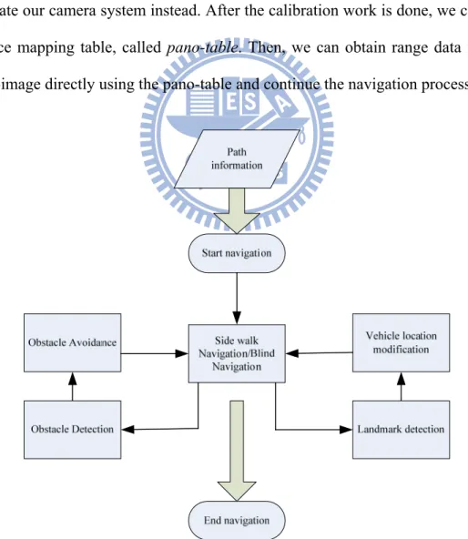
B. The navigation stage
In the navigation stage, with the path information learned in advance, an automatic navigation process is started. Three major works are conducted by the vehicle in the navigation process moving forward, obstacle detection, and vehicle location modification.
In principle, the autonomous vehicle constantly move forward toward the goal node by node based on the learned path information. In the movement between any two nodes in the path, the vehicle chooses one of two navigation modes navigation by following the sidewalk or navigation just by the use of an odometer (called the blind navigation mode). When navigating in the first mode, the sidewalk curb with a
prominent color is detected continuously and the line following technique is adopted to guide the vehicle. When no curb can be used for line-following guidance as often encountered on sidewalks, the second mode is adopted in which the vehicle navigates blindly according to the information of the odometer reading and the learned path.
Also, as a rule, the autonomous vehicle tries to find obstacles at any time and can take a proper obstacle avoidance strategy when desired. By the use of a stereo omni-camera, we develop a new method to detect obstacles on the ground using computer vision techniques. Moreover, when reaching a particular location in the learned path, the autonomous vehicle will detect the appointed landmark to localize itself automatically.
Furthermore, in this study we use some objects such as hydrants and light poles, which often can be found on sidewalks, as landmarks for vehicle localization. That is, we modify the vehicle position with respect to each located landmark to eliminate cumulated mechanical or vision-processing errors during the navigation process. Specifically, we propose a new space line detection technique to detect the along-path hydrant and the light pole and then calculate the locations of them. By these
techniques, the autonomous vehicle can navigate safely and smoothly to the
destination at the end of the navigation stage.
1.4 Contributions of This Study
Some contributions of this study are described as follows.1. A method of training an autonomous vehicle for outdoor navigation using commonly-seen objects on sidewalks is proposed.
2. A new space line detection and localization technique using the pano-mapping table is proposed.
3. Techniques for detecting hydrants and light poles as landmarks for vehicle localization are proposed.
4. A technique of following sidewalk curbs for vehicle navigation is proposed. 5. A new obstacle avoidance technique and a new camera calibration method for it
are proposed.
6. Dynamic camera exposure adjustment and dynamic thresholding methods for use in outdoor environments are proposed.
1.5 Thesis Organization
The remainder of this thesis is organized as follows. In Chapter 2, we introduce the configuration of the proposed system and the system process in detail. In Chapter 3, the proposed training methods for vehicle to learn the guidance parameters and the navigation path are described. In Chapter 4, we introduce the navigation strategies including the ideas, the proposed guidance techniques, and detailed navigation algorithms. In Chapter 5, a new space line technique is proposed and the proposed techniques of hydrant and light pole detections are described. In Chapter 6, the navigation techniques of line following and obstacle avoidance are introduced. In Chapter 7, some experimental results to show the feasibility of the proposed techniques for vehicle navigation are shown. At last, conclusions and some suggestions for future works are given in Chapter 8.
Chapter 2
System Design and Processes
2.1 Idea of System Design
For a blind person to walk safely on a sidewalk, a vision-based autonomous vehicle system is a good substitute for a guide dog, as mentioned previously. Because of the advantages of possessing good mobility and long-time navigation capabilities, autonomous vehicles have become more and more popular in recent years for many applications. Equipped with cameras, an autonomous vehicle is able to “see” like a human being. Moreover, both the autonomous vehicle and the cameras may be connected to a main control system, which have the capabilities to integrate information, analyze data, and make decisions. In this study, we have designed an autonomous vehicle system of this kind for use as a machine guide dog. The entire configuration of the system will be introduced in detail in Section 2.2, and 3D data acquisition using the camera will be described in Section 2.3.
In an unknown environment, the autonomous vehicle system still has to be “trained” before it can navigate by itself. Specifically, it should be “taught” to know the information of the navigation path; how to navigate in this path; and how to handle different conditions on the way. Moreover, secure navigation strategies should also be established for the vehicle to protect the blind and itself. In the end, the vehicle should be able to navigate in the same path repetitively with the learned data and the navigation strategies. The system processes designed to achieve these functions on the proposed autonomous vehicle system will be described in Section 2.3,
including the learning process described in Section 2.3.1 and the navigation process in Section 2.3.2.
2.2 System Configuration
In this section, we will introduce the configuration of the proposed system. We use Pioneer 3, an intelligent mobile vehicle made by MobileRobots Inc. as shown in Figure 2.1, as a test bed for this study. The autonomous vehicle and other associated hardware devices will be introduced in more detail in Section 2.2.1. In addition, a particularly-designed stereo omni-camera is employed in this study and equipped on the autonomous vehicle. We will describe the structure of the camera system in Section 2.2.2. Finally, the configuration of the software we use as the development tool will be introduced in Section 2.2.3.
Figure. 2.1 Autonomous vehicle, Pioneer 3 produced by MobileRobots Inc., used in this study.
2.2.1 Hardware configuration
The hardware architecture of the proposed autonomous vehicle system can be divided into three parts. The first is the vehicle system; the second the camera system,
and the third the control system. The latter two are installed on the first, the vehicle system, as shown in Figure 2.2. We will introduce these systems one by one subsequently.
(b)
(a)
(c)
Figure. 2.2 Three different views of the used autonomous vehicle, which includes a vehicle, a stereo camera, and a notebook PC for use as the control unit. (a) A 45o view. (b) A front view. (c) A side view.
The vehicle, Pioneer 3, has an aluminum body with the size of 44cm×38cm× 22cm, two wheels of the same diameter of 16.5cm, and one caster. Also, 16 ultrasonic sensors are installed on the vehicle, half of them in front of the body and the other half behind. When navigating on flat floors, Pioneer 3 can reach its maximum speed 1.6 meters per second. Also, it has the maximum rotation speed of 300 degrees per second, and can climb up a ramp with the largest slope of 30 degrees. The vehicle is able to
carry payloads up to 23kg at a slower speed. It has three 12V rechargeable lead-acid batteries and can run constantly for 18 to 24 hours if all of the batteries are fully charged initially. The vehicle also provides the user some parameter information of the system, such as the vehicle speed, the battery voltage, etc.
The camera system, called a two-mirror omni-camera, consists of one perspective camera, one lens, and two reflective mirrors of different sizes. The perspective camera, ARCAM-200SO, is produced by the ARTRAY company with a size of 33mm×33mm×50mm and the maximum resolution of 2.0M pixels. With the maximum resolution, the frame rate can reach 8 fps. The CMOS visual sensor in the camera has a size of 1/2 inches (33mm×33mm). The lens is produced by Sakai Co. and has a variable focal length of 6-15mm. The two reflective mirrors are produced by Micro-Star International Co. A detailed view of the entire camera system is shown in Figure. 2.3, and the camera and the lens are shown in Figures 2.3(a) and 2.4(b), respectively. Other details about the camera structure will be described in the next section.
(a) (b) Figure. 2.3 The two-mirror omni-camera used in this study. (a) A full view of the camera equipped
About the final part, we use a laptop computer as the control system. It is of the model of ASUS W7J produced by ASUSTek Computer Inc. as shown in Figure. 2.5. For the computer to communicate with the other parts, we connected it with the autonomous vehicle by an RS-232, and with the camera system by a USB.
(a) (b) Figure. 2.4 The used camera and lens. (a) The camera of model Arcam 200so produced by ARTRAY
Co. (b) The lens produced by Sakai Co.
Figure. 2.5 The laptop computer of model ASUS W7J used in this study.
2.2.2 Structure of used two-mirror omni-camera
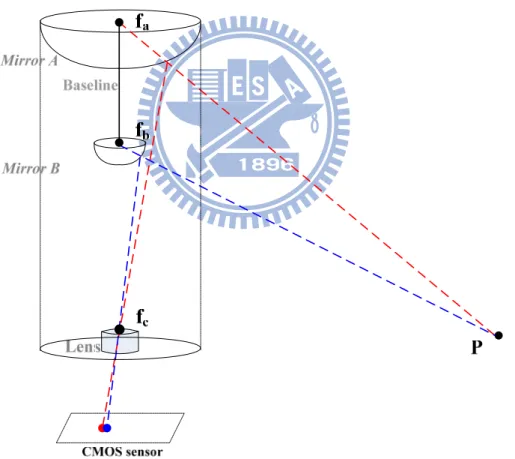
The structure of the two-mirror omni-camera used in this study and the projection of a space point P onto the system are illustrated in Figure 2.6. We call the
bigger and higher mirror Mirror A, and the smaller and lower one Mirror B subsequently, and both of them are made to be of the shape of a hyperboloid with parameters shown in Table 2.1. One of the focal points of Mirror A is on fa and one of
the focal points of Mirror B is on fb. Both mirrors have another focal point on the
same position fc which is the center of the lens. In addition, the line segment ,
which we call the baseline, has a length in 20cm.
a b
f f
Table 2.1 Specifications of the used two hyperboloidal-shaped mirrors.
radius Parameter a Parameter b
Mirror A 12 cm 11.46cm 9.68cm
Mirror B 2cm 2.41cm 4.38cm
An important optical property of the hyperboloidal-shaped mirror is: if a light ray goes through one focal point, it must be reflected by the mirror to the other focal point. As illustrated in Figure 2.7, two light rays which go through fa and fa are both
reflected to the same focal point fc by the specially-designed mirrors, Mirrors A and B,
respectively. Based on these property of the omni-camera and as illustrated in Figure 2.6, a space point P will be projected onto two different positions in the CMOS sensor in the camera along the blue light ray and the red light ray reflected by Mirrors A and B, respectively, so that the range data of P can be computed according to the two resulting distinct image points.
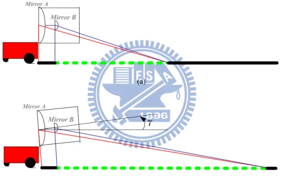
Furthermore, the way of placement of the two-mirror omni-camera on the vehicle has been carefully considered. The camera was originally placed in such a way that the optical axis going through Mirrors A and B is parallel to the ground as shown in Figure 2.8(a). In the omni-image acquired by the two-mirror omni-camera,
because of the existence of the image region caused by Mirror B, the image region of the field of view (FOV) reflected by Mirror A became smaller. We can see that the overlapping region on the ground where range data can be computed was not large enough in this situation (as shown in the green dotted region in the figure). However, for a navigation system, the front FOV is very important for the vehicle to avoid collisions. Moreover, it is desired that the vehicle can find obstacles at distances as large as possible in the navigation process. Due to these reasons, the camera was later slanted up for an angle of as shown in Figure 2.8(b). We can see in the figure that the region of overlapping is now bigger than before.
Figure 2.6 The prototype of the two-mirror omni-camera and a space point projected on the CMOS sensor of the camera.
Figure 2.7 The reflection property of the two hyperboloidal-shaped mirrors in the camera system.
(a)
Mirror A
Mirror B
(b)
Figure 2.8 Two different placements of the two-mirror omni-camera on the vehicle and the region of overlapping. (a) The optical axis going through the two mirrors is parallel to the ground. (b) The optical axis through the two mirrors is slanted up for an angle of .
2.2.3 Software configuration
The producer, MobileRobots Inc., of the autonomous vehicle used in this study provides an application interface, called ARIA (Advanced Robotics Interface Application), for the user to control the vehicle. The ARIA is an object-oriented
interface which can be used under the Win32 or Linux operating system using the C++ language. Therefore, we can utilize the ARIA to communicate with the embedded sensor system in the vehicle and obtain the vehicle state to control the pose of the vehicle.
For the camera system, the ARTAY provides a development tool called Capture Module Software Developer Kit (SDK). This SDK is an object-oriented interface and its application interface is written in several computer languages like C, C++, VB.net, C#.net and Delphi. We use the SDK to capture image frames with the camera and can change many parameters of the camera, such as the exposure. In the control system, we use Borland C++ Builder 6, which is a GUI-based interface development environment, to develop our system processes on the Windows XP operating system.
2.3 3D Data Acquisition by the
Two–mirror Omni-camera
2.3.1 Review of imaging principle of the two-mirror
omni-camera
Before derivation of the formulas for range data computation by the use of the two-mirror omni-camera, we review first the imaging principle of a simple omni-camera consisting of a hyperboloidal-shaped mirror and a projective camera. First of all, we introduce two coordinate systems as shown in Figure 2.9 where the image coordinate system (ICS) is a two-dimensional coordinate system coincident with the omni-image plane with its origin being the center of the omni-image. The camera coordinate system (CCS) in Figure 2.9 is a three-dimensional coordinate system with the origin being located at a focal point of the mirror.
According to the optical property of the hyperboloidal-shaped mirror, a space point P at coordinates (x, y, z) in the CCS is projected onto an omni-image point I at coordinates (u, v) in the ICS as shown in Figure 2.9. In more detail, assume that a light ray from P goes through a focal point in the mirror center Om. Then, reflected by
the hyperboloidal-shaped mirror, the light ray goes through another focal point at the lens center Oc. It is finally projected onto an image point I at coordinates (u, v) on the
image plane. In this way of imaging space points, therefore, for each image point I, we can find a corresponding light ray with a specific elevation angle and a specific azimuth angle θ (shown in the figure by the red and the green characters, respectively) to represent the image point I.
Figure 2.9 Imaging principle of a space point P using an omni-camera.
2.3.2 3D data computation for used two-mirror
omni-camera
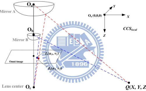
omni-camera, we define a camera coordinate system (CCS) as shown in Figure 2.10. The origin of is the focal point of Mirror A, and the Z-axis coincident with the optical axis going through the two mirrors. As shown in the figure, there is a space point Q at coordinates (X, Y, Z) in CCS which is projected respectively by the two mirrors onto two image points, Is at coordinates (u1, v1) and Ib
at coordinates (u2, v2), in the omni-image. By the geometry of the camera oprtics, we
may compute the 3D position of Q by the following way.
local CCS cal local CCS lo Oa Q(X, Y, Z) Omni-image Mirror A Mirror B Lens center Oc Ob Is(u1, v1) Ib(u2,v2) CCSlocal Oa (0,0,0) Z X Y
Figure 2.10 The cameras coordinate system , and a space point Q projected on the omni-image acquired by the two-mirror omni-camera.
local
CCS
Firstly, following the two light rays which go through Mirror A’s center and Mirror B’s center, respectively, we obtain two different elevation angles a and b as shown in Figure 2.11(a). Also, the points Oa,Ob, and Q form a triangle OaObQ which we
especially illustrate in Figure 2.11(b). The distance between Oa and Ob, which is the
length of the baseline defined previously, is known to b, while the distance d between Oa and Q is an unknown parameter. By the law of sines based on geometry, we can
sin(90o ) sin( ) b b d b ; (2.1) sin(90 ) sin( ) o b b b d . (2.2)
d
Oa Q Ob 90o αa 90o αb αa-αbb
(a) (b) Figure 2.11 An illustration of the relation between a space point Q and the two mirrors in the usedSecondly, we may compute the azimuth angles of the two light rays. According to the
s
1 1
camera. (a) A side view of Q projected onto the two mirrors. (b) A triangle OaObQ used in deriving 3D data.
property of rotational invariance of the omni-image, these two azimuth angles actually are equal, which we denote by . From Figure 2.12, by the use of the image point I at coordinates (u , v ), we can derive θ by the following equations:
1 1 2 2 2 2 1 1 1 1 sin u ; cos v u v u v ; 1 1 1 1 2 2 2 2 1 1 1 1 sin ( u ) cos ( v ) u v u v . (2.3)
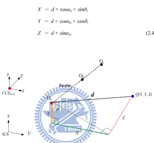
Thirdly, with the distance d derived by Equation (2.2) and the azimuth angle θ obtained by Equation (2.3), we can compute the position of Q in according to geometry illustrated in Figure 2.12 as follows:
local
CCS
X = d × cosαa × sinθ,
Y = d × cosαa × cosθ,
Z = d × sinαa. (2.4)
Figure 2.12 An illustration of a space point Q at coordinates (X, Y, Z) in CCSlocal.
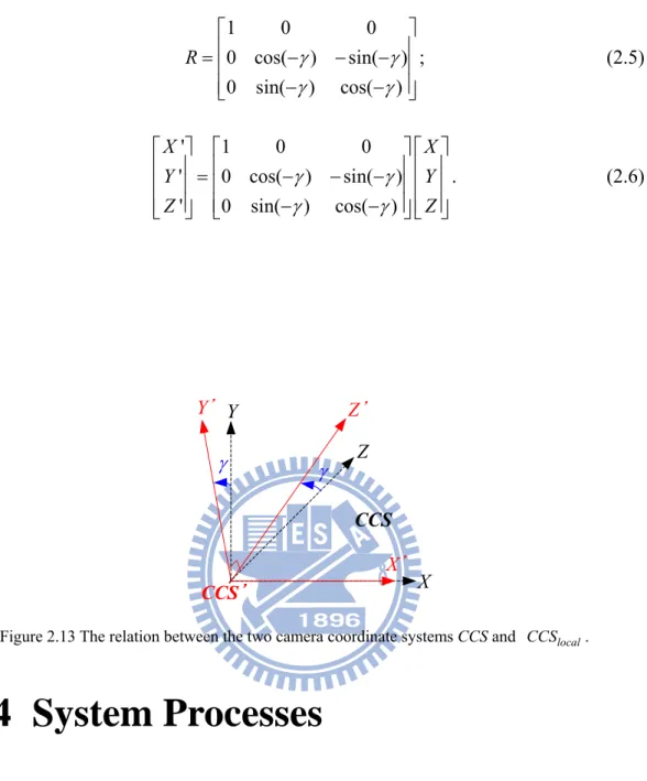
However, as mentioned previously, the optical axis going through the two mirrors is slanted up so that it is not parallel to the ground. It is desired that the Z-axis
of could be parallel to the ground. As shown in Figure 2.13, we define
another camera coordinate system CCS, which coincidences w Slocal except
that the Z-axis is slanted for an angle of toward the Y-axis along the X-axis. Finally, the coordinates of Q is translated to a new coordinates (X’, Y’, Z’), which we want to obtain, in the CCS by the use of a rotation matrix R by following equations:
local
CCS
1 0 0 0 cos( ) sin( ) 0 sin( ) cos( ) R ; (2.5) ' 1 0 0 ' 0 cos( ) sin( ) ' 0 sin( ) cos( ) X X Y Y Z Z . (2.6) Z Y Z X CCS CCS X Y
Figure 2.13 The relation between the two camera coordinate systems CCS and CCSlocal.
2.4 System Processes
2.4.1 Learning process
The goal in the learning process is to “teach” the autonomous vehicle to know how to navigate automatically in a pre-specified path. The entire learning process proposed in this study is shown in Figure 2.14. Discussed in the following is some information which the vehicle should “memorize.” First, as mentioned in Chapter 1, the autonomous vehicle has to conduct self-localization by some pre-selected landmarks in the specified path, so the first type of information the vehicle have to record is the landmark locations along the path. Next, for our study, the experimental
environment is on the sidewalk, and this has an advantage that the vehicle may navigate along the curb of the sidewalk. For this reason, line following along the sidewalk curb, called sidewalk following, is a proper navigation method instead of using the odometer only. Thus, the second type of information which has to be recorded is the vehicle navigation information along the path (path nodes, the navigation distance between two nodes, etc.). Finally, the environment information at different locations on the navigation path also has to be recorded.
For the purpose of training an autonomous vehicle easily, a user learning interface is constructed for the trainer and can be used to control the autonomous vehicle as well as construct learning navigation information. First, at the beginning of each section of the navigation path, the trainer should establish a set of corresponding navigation rules in advance, and the vehicle will follow them and conduct navigation in the learning process as well as in the navigation process. Then, the current vehicle pose obtained from the odometer and some current environment information like the illumination are also recorded. Next, when the mode, navigation by following the sidewalk, is selected, a semi-automatic learning process will proceed until reaching the next node assigned by the trainer. Otherwise, the trainer is required to guide the vehicle manually to the next path node by the use of the learning interface.
In addition, the trainer can decide where to localize the vehicle by a selected landmark in the learning process. After guiding the vehicle to a proper pose for detecting the landmark (close enough to the landmark, “looking” at the landmark from the right direction, etc.), the trainer then has to establish relevant rules for landmark detection. Some parameters for landmark detection can be appropriately adjusted by the trainer before the detection work is started. Next, landmark localization is conducted by a space line detection technique described in Chapter 5. After possibly multiple times of detecting and collecting adequate information of the
landmark, its position is finally computed automatically and recorded.
At last, after bringing the autonomous vehicle to the destination, the learning process is finished, and the learned information is organized into a learned path composed of several path nodes with guidance parameters. Combining it with landmark information and environment information, we obtained an integrated path map which finally is stored in the memory of the vehicle navigation system.
2.4.2 Navigation process
With the map information obtained in the learned process, the autonomous vehicle can continually analyze the current location using various stored information and navigate to an assigned goal node on the learned path in the navigation process. The entire navigation process proposed in this study is shown in Figure 2.15.
According to the learned information data retrieved from the storage, the autonomous vehicle continually analyzes the current environment node by node to navigate to the goal. At first, before starting to navigate to the next node, the autonomous vehicle checks if the image frame is too dark or too bright according to the learned environment parameter data, and then dynamically adjusts the exposure of the camera if necessary.
After that, the autonomous vehicle always checks if any obstacle exists in front of the vehicle. As soon as an obstacle is found and checked to be too close to the vehicle, a procedure of collision avoidance is started automatically to perform collision avoidance. Then, based on the learned navigation rules, the autonomous vehicle checks the corresponding navigation mode and follows it to navigate forward. In the meantime, the vehicle checks whether it has arrived at the next node; whether the node is the destination; or whether the vehicle has to localize its current position.
Learning of landmarks Learning of
environment Learning of navigation
path
User learning interface
Start of learning Eestablish navigation rules Eestablish landmark deteciton rules Manual navigate vehicle Detect landmarks End of learning Automatic sidewalk following Create navigation map Vehicle odometer Landmark localization Learning information Map information Vehicle navigation information Landmark location analysis Landmark information Environment information
Figure 2.14 Learning process.
In addition, if a self-localization node is expected, the autonomous vehicle will adjust its pose and relevant parameters into an appropriate condition and conduct landmark detection. For landmark detection, the autonomous vehicle uses the corresponding technique in accordance with the property of the landmark. If a desired landmark is found and localized successfully, its location then is used to modify the position of the vehicle; if not, some remedy for recovering the landmark will be conducted, such as changing the pose of the vehicle to detect the landmark again.
Chapter 3
3.1.1
3.1.2
Learning Guidance Parameters and
Navigation Paths
3.1 Introduction
Before the autonomous vehicle can navigate, some works has to be conducted in the learning process. First, the camera system should be calibrated. Then, a path and a set of landmarks should be selected, and each landmark location should be recorded into the path, resulting in a learned path. Finally, adopted guidance parameters have to be “trained” and then recorded.
Camera calibration
As mentioned in Chapter 1, instead of calibrating the camera’s intrinsic and extrinsic parameters, we adopt a space-mapping technique [25], called pano-mapping, to calibrate the two-mirror omni-camera used in this study. We will describe the adopted technique in Section 3.2.
Selection of landmarks for navigation guidance
For the purpose to localize the position of the vehicle during the navigation process, some objects should be selected as landmarks to conduct vehicle localization. Two types of objects, hydrant and light pole, as shown in Fig 3.1 are selected in this study as landmarks for vehicle localization during sidewalk navigation. By the use of proposed hydrant and light pole localization techniques, introduced later in Chapter 5,
we can guide the vehicle to learn the positions of pre-selected hydrants and light poles in the learning process.
Figure 3.1 The hydrant (left) and the light pole (right) used as landmarks in this study.
3.1.3 Learning of guidance parameters
For complicated outdoor environments, the trainer should train some parameters for use in vehicle guidance, such as environment parameters and image segmentation thresholds, in the learning process. We will introduce the proposed techniques for learning environment parameters in Sections 3.4. Also, some image segmentation parameters for landmark image analysis and the techniques proposed to learn them will be introduced in Sections 3.5. Finally, a scheme proposed to create the learned navigation path will be described in Section 3.6.
3.2 Camera Calibration by
Space-mapping Approach
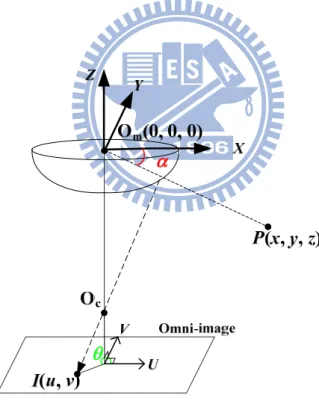
We utilize the pano-mapping technique proposed by Jeng and Tsai [25] for image unwarping to calibrate the camera system used in this study. The main idea is to establish a so-called pano-mapping table to record the relation between image points and corresponding real-world points. More specifically, as illustrated in Figure 3.2, a
light ray going through a world-space point P with the elevation angle α and the azimuth angle θ is projected onto a specific point p at coordinates (u, v) in the omni-image. The pano-mapping table specifies the relation between the coordinates (u, v) of the image point p and the azimuth-elevation angle pair ( of the corresponding world-space point P. The table is established in advance and can be looked up to retrieve 3D information forever. Accordingly, we construct two pano-mapping tables for Mirrors A and B, respectively, by the following steps, assuming an omni-image I has been taken as the input.
Algorithm 3.1 Construction of pano-mapping tables.
Step 1. Manually select in advance six known image points pi at coordinates (ui, vi,) on the Mirror A region in omni-image I and the six corresponding known world-space points Pi at coordinates (xi, yi, zi), where i is 1 through 6.
Step 2. Select similarly six known image points qj at coordinates (Uj, Vj,) on the Mirror B region in omni-image I and the six corresponding known world-space points Qj at coordinates (Xj, Yj, Zj), where j is 1 through 6. Step 3. For image points pi and qj, compute the radial distances ri and Rj in the
image plane with respect to the image center respectively by the following equations:
2 2; 2 2
i i i i i i
r u v R U V . (3.1)
Step 4. Compute the elevation angles αi and βi for the corresponding world-space points Pj and Qj by the following equations:
2 2 2 2 1 1 tan ( / ); tan ( / ) i zi xi yi i Zi Xi Y i (3.2)
for Mirrors A and B, respectively.
Step 5. Under the assumption that the surface geometries of Mirrors A and B are radially symmetric in the range of 360 degrees, use two radial stretching functions, denoted as fA and fB, to describe the relationship between the radial distances ri and the elevation angles αi as well as that between Rj and βj, respectively, by the following equations:
1 2 3 4 0 1 2 3 4 5 ( ) i A i i i i i r f a a a a a a i5 5 i ; 1 2 3 4 0 1 2 3 4 5 ( ) i B i i i i i R f b b b b b b . (3.3)
Step 6. Solve the above 6-th degree polynomial equations fA and fB by the use of the six radial-distance pairs for Mirrors A and B, respectively, obtained in Step 4 using a numerical method to obtain the coefficients a0 through a5 and b0
through b5.
Step 7. By the use of the function fA with the known coefficients a0 through a5,
construct the pano-mapping table for Mirror A in a form as that shown in Figure 3.3(a) according to the following rule:
for each world-space point Pij with the azimuth-elevation pair (θi, αj), compute the corresponding image coordinates (uij, vij) by the following equations:
cos ; sin
ij j i ij j i
u r v r . (3.4)
Step 8. In a similar way, construct the pano-mapping table for Mirror B by the use of the function fB with the known coefficients b0 through b5 in a form as that
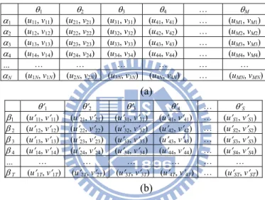
Figure 3.2 The relation between a space point P and the relevant elevation angle and azimuth. 1 2 3 4 … M 1 (u11, v11) (u21, v21) (u31, v31) (u41, v41) … (uM1, vM1) 2 (u12, v12) (u22, v22) (u32, v32) (u42, v42) … (uM2, vM2) 3 (u13, v13) (u23, v23) (u33, v33) (u43, v43) … (uM3, vM3) 4 (u14, v14) (u24, v24) (u34, v34) (u44, v44) … (uM4, vM4) … … … N (u1N, v1N) (u2N, v2N) (u3N, v3N) (u4N, v4N) … (uMN, vMN) (a) 1 2 3 4 … S 1 (u11, v11) (u21, v21) (u31, v31) (u41, v41) … (uS1, vS1) 2 (u12, v12) (u22, v22) (u32, v32) (u42, v42) … (uS2, vS2) 3 (u13, v13) (u23, v23) (u33, v33) (u43, v43) … (uS3, vS3) 4 (u14, v14) (u24, v24) (u34, v34) (u44, v44) … (uS4, vS4) … … … T (u1T, v1T) (u2T, v2T) (u3T, v3T) (u4T, v4T) … (uST, vST) (b)
Figure 3.3 Two pano-mapping tables used for the two-mirror omni-camera used in this study. (a) Pano-mapping table used for Mirror A. (b) Pano-mapping used for Mirror B.
3.3 Coordinate Systems
In this section, we will introduce the coordinate systems used in this study, which describe the relations between the used devices and concerned landmarks in the navigation environment. Furthermore, the used odometer and some involved coordinate transformations are introduced also. The following are four coordinate systems used in this study.
(2). Vehicle coordinate system (VCS): denoted as (VX, VY). The VX-VY plane coincides with the ground and the origin OV of the VCS is located at the center
of the autonomous vehicle.
(3). Global coordinate system (GCS): denoted as (MX, MY). The MX-MY plane coincides with the ground. The origin OG of this system is always placed at the
start position of the vehicle in the navigation path.
(4). Camera coordinated system (CCS): denoted as (X, Y, Z). The origin OC of the
CCS is placed at the focal point of Mirror A. The X-Z plane is parallel to the ground and the Y-axis is perpendicular to the ground.
Navigation Environment
M
XO
GM
Y (a) (b) Figure 3.4 Two coordinate systems used in this study. (a) The ICS. (b) The GCS.In this study, the navigation path is specified by the GCS as shown in Figure 3.4(b). The relationship between the GCS and the VCS is illustrated in Figure 3.5. At the beginning of the navigation, the VCS coincides with the GCS, and then the VCS follows the movement of the current vehicle position as well as the CCS. In addition, it is emphasized that the vehicle uses an odometer to localize its position in the GCS. As illustrated in the figure, the reading of the vehicle odometer is denoted as (Px, Py, Pth) where Px and Py represent the current vehicle position with respect to its original
position on the ground, and Pth represents the rotation angle of the vehicle axis with respect to the GCS.
As shown in Figure 3.6, assume that the vehicle is at a position V at world coordinates (Cx, Cy) with a rotation angle θ. We can derive the coordinate transformation between the coordinates (MX, MY) of the VCS and the coordinates (VX, VY) of the GCS by the following equations:
cos sin X X Y x M V V C ; sin cos Y X Y y M V V C . (3.5)
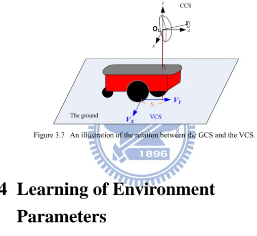
In addition, the relationship between the CCS and the VCS is illustrated in Figure 3.7. As shown in the figure, the projection of the origin of the CCS onto the ground does not coincident with the origin of the VCS, and there is a horizontal distance between the two origins, which we denote as Sy. Thus, the coordinate transformation between the CCS and the VCS can be derived in the following way:
;
X
V X VY Z Sy. (3.6)
Figure 3.6 A vehicle at coordinates (Cx, Cy) with a rotation angle θ with respect to the GCS.
Figure 3.7 An illustration of the relation between the GCS and the VCS.
3.4 Learning of Environment
Parameters
3.4.1 Definition of environment windows on images
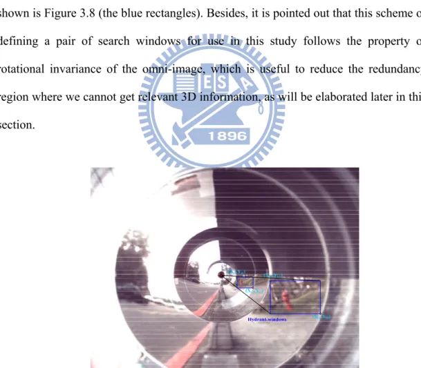
In the process of navigation, the vehicle conducts several works including following sidewalk curbs, finding landmarks, obstacle detection, etc. In general, each desired landmark is projected onto a specific region in the image. By this property, we can consider only the region of interest in the image instead of the whole image, and two advantages can be obtained from this approach as follows: