Bound state of the quantum dot formed at intersection of L- or T-shaped quantum wire in inhomogeneous magnetic field

(1)

Bound state of the quantum dot formed at intersection of L- or T-shaped quantum wire

in inhomogeneous magnetic field

Yuh-Kae Lin, Yueh-Nan Chen, and Der-San Chuu

Citation: Journal of Applied Physics 91, 3054 (2002); doi: 10.1063/1.1446233 View online: http://dx.doi.org/10.1063/1.1446233

View Table of Contents: http://scitation.aip.org/content/aip/journal/jap/91/5?ver=pdfcov

Published by the AIP Publishing

Articles you may be interested in

Quantum transport through the system of parallel quantum dots with Majorana bound states

J. Appl. Phys. 115, 083706 (2014); 10.1063/1.4867040

Tunneling transport through multi-quantum-dot with Majorana bound states

J. Appl. Phys. 114, 033703 (2013); 10.1063/1.4813229

Electrically induced bound state switches and near-linearly tunable optical transitions in graphene under a magnetic field

J. Appl. Phys. 109, 104306 (2011); 10.1063/1.3583650

Bound states in a hybrid magnetic-electric quantum dot

J. Appl. Phys. 108, 064306 (2010); 10.1063/1.3486495

Bound states for an induced electric dipole in the presence of an azimuthal magnetic field and a disclination

J. Math. Phys. 51, 093516 (2010); 10.1063/1.3490192

(2)

Bound state of the quantum dot formed at intersection of

L

- or

T

-shaped

quantum wire in inhomogeneous magnetic field

Yuh-Kae Lin, Yueh-Nan Chen, and Der-San Chuua)

Department of Electrophysics, National Chiao Tung University, 1001 Ta Hsueh Road, Hsinchu, 30050 Taiwan

共Received 30 May 2001; accepted for publication 30 November 2001兲

A quantum dot 共QD兲 can be formed at the intersection of the symmetric or asymmetric L-shaped 共LQW兲 or T-shaped quantum wire 共TQW兲. The bound state energies in such QD systems surrounded by inhomogeneous magnetic fields are found to depend strongly on the asymmetric parameter ␣ ⫽W2/W1, i.e., the ratio of the arm widths and magnetic field applied on the wire arms. Two effects

of the magnetic field on the bound state energy of the electron can be obtained. One is the depletion effect which purges the electron out of the QD system. The other is to create an effective potential due to the quantized Landau levels of the magnetic field. Depletion effect is found to be more prominent in weak field region. Our results show the bound state energy of the electron in such QD system depends quadratically共linearly兲 on the magnetic field in the weak 共strong兲 field region. It is also found that the bound state energy of the electron depends on the magnetic field strength only and not on its direction. A simple model is proposed to explain the behavior of the magnetic dependence of the bound state energy of the electron both in weak and strong magnetic field regions. The contour plots of the relative probability of the bound state in LQW or TQW in magnetic field are also presented. © 2002 American Institute of Physics. 关DOI: 10.1063/1.1446233兴

I. INTRODUCTION

The mesoscopic structures of semiconductors have at-tracted intensive studies because they exhibit physical phe-nomena and concepts that are important in future applica-tions of electronic devices. By mesoscopic structure, we mean the dimension of the system is less than or comparable to the phase-breaking length of the conduction electrons and much larger than the microscopic objects. Recently, quasi-one-dimensional structures, such as quantum wires attract much attention due to the enhanced confinement of the re-duced dimension and the possibility of tailoring the elec-tronic and optical properties in applications.1–18The physics describing the phenomena of quantum interference devices has to be explored before the development of technology. Among the structures considered, the quantum dot 共QD兲 is one of the simpler mesoscopic systems in which the essential physics can be studied in great details. A QD can be defined by additional lateral confinements19,20or by applying certain magnetic fields.21,22The QD can also be formed at the inter-section of the arms of a L-shaped 共LQW兲 or a T-shaped 共TQW兲 quantum wire when additional magnetic fields are applied on the arms. These QDs are quite different from the traditional quantum dots, since there remain openings in such QDs. Electrons in such QD systems are classically un-bounded. However, recent experimental photoluminescence spectroscopy analyses4 – 6 have manifested that there are bound states in such QDs. The existence of bound states in such QDs essentially shows the confinement effect of the mesoscopic geometry in quantum mechanical region. In

ad-dition, the stationary states of a charged particle 共e.g., elec-tron兲 in such QDs are affected by the applications of the inhomogeneous magnetic fields.

The exploration of the properties of bound states is a key to understand some recent optical and electrical experiments on T-shaped quantum wires and quantum dots.5–7,15,18 –20The magnetophotoluminescence of T-shaped wires were mea-sured recently.9The energy shift ⌬E of photoluminescence peaks with magnetic field B applied perpendicular to the wire axis and parallel to the stem wire was measured. In these experiments, the information of exciton binding energy can be provided from the photoluminescence spectroscopy. How-ever, it is unable to identify exactly the exciton binding ergies unless we have the knowledge of the confinement en-ergy of either an electron or a hole in quantum wires or quantum dots. Because they cannot be extracted directly from magneto-optical data due to the nonlinearity of the sys-tems. In a theoretical calculation of magnetoexcitons in

T-shaped wires,23the observed field dependence of the exci-ton states for weak confinement was reproduced, however, the diamagnetic shifts calculated from perturbation theory is fail to describe the experimental results.

In typical semiconductors, the effective masses of holes are generally anisotropic in two dimensions. Through proper variable transformation, the problem of anisotropic effective mass can be transformed formally into a problem with asym-metric geoasym-metric structure but with isotropic effective mass. However, the anisotropic effect is an intrinsic property which can be resulted only from the lattice composition, while the asymmetric effect is an extrinsic one due to the fabrication of the crystal. And this extrinsic asymmetry is often able to provide a larger preferable variation range of bound state energies whilst the intrinsic anisotropy could not. Therefore, a兲_{Author to whom correspondence should be addressed; electronic mail:}

dschuu@cc.nctu.edu.tw

3054

(3)

through understanding the asymmetric effect, it might be-come easier to correctly tailor the devices at our desire.

In this work, we study the effects of the asymmetric geometry and the surrounding inhomogeneous magnetic fields on the electronic bound state in QDs formed in a two-dimensional L-shaped and T-shaped quantum wires. A

T-shaped quantum wire can be obtained by first growing a

GaAs/AlxGa1_⫺xAs superlattice on a 共001兲 substrate, after

cleavage, a GaAs quantum wire is grown over the exposed 共110兲 surface, resulting in a T-shaped region where the elec-tron or hole can be confined on a scale of 5–10 nm. The bound state energy of a charged particle 共e.g., electron兲 in such a quantum dot will be affected by the asymmetric ge-ometry of the system and the applied inhomogeneous mag-netic fields. Intuitively, when the confinement along one arm of the quantum wire is increased, either by decreasing the arm width or by allowing the magnetic fields surrounded the QD to change, confinement along the orthogonal arm will decrease, because squeezing the electron or hole in one arm will result in pushing the electron or hole out of the quantum wire through the other arm. These phenomena are not only interesting in physics but also have no classical correspon-dence. This squeezing effect has not been studied thoroughly. Furthermore, T-shaped semiconductor quantum wires could be exploited as three-terminal quantum interference devices, thus the study on the L-shaped or T-shaped quantum wire is also important in practical applications. Our model will be presented briefly in the next section. Results and discussions will be given in the final section.

II. FORMULATION

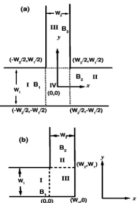
We consider QDs formed in a two-dimensional TQW or LQW. In our treatment the thickness in the z direction of our system is assumed to be very small while compared to the other two directions. Therefore, it could be practically con-sidered as a two-dimensional system. The confinement ex-isted in the z direction makes the separation of the sublevels in z-direction of our system to be very large while compared to those sublevels in the x and y directions of our system. The TQW and LQW are consisted of a horizontal arm and a vertical arm, lying on the X – Y plane. The TQW can be divided into four uniform subregions: a horizontal arm with a width of W1 共region I兲 to which a magnetic field B1 is

ap-plied perpendicularly, another horizontal wire with a width of W1 共region II兲 to which a magnetic field B2 is applied

perpendicularly, a vertical arm with a width of W2 to which

a magnetic field B3 is also applied perpendicularly and an

intersection region with an area of W1⫻W2 共region IV兲, as

shown in Fig. 1共a兲. For simplicity, the boundaries are as-sumed to be a hard-wall confinement potential, leading to the formation of a magnetically confined cavity in which the confinement of electron is enhanced. The case of LQW 关shown in Fig. 1共b兲兴 can be regarded as a transformation of TQW in which the arm 2 is cutoff and only three subregions are left. The transverse potential inside the TQW or LQW is assumed to be zero. For further studies, the magnetic fields are assumed to be uniform in each individual subregion and is zero in the intersection region 共region IV兲. Within the framework of effective mass approximation, the Schro¨dinger equation of an electron in TQW system共the system of LQW is just the special situation of TQW兲 under an inhomoge-neous magnetic field can be expressed as:

冋

⫺共p⫺qA共x,y兲兲

2

2m* ⫹Vc共x,y兲

册

⌿共x,y兲⫽E⌿共x,y兲, 共1兲

where m* and q are the effective mass and the charge of the particle, Vc(x, y ) is the confinement potential, and p is the

momentum, A„x,y… is the vector potential associated with the magnetic fields. To solve the equation, the Landau gauge is chosen for the vector potential in different subregions as

A„x,y…⫽

冦

关0,B1共x⫹0.5W2兲兴⫽共⫺B1y ,0兲⫹ⵜB1共x⫹0.5W2兲y, in region I;

关0,B2共x⫺0.5W2兲兴⫽共⫺B2y ,0兲⫹ⵜB2共x⫺0.5W2兲y, in region II;

关⫺B3共y⫺0.5W1兲,0兴⫽共0,B3x兲⫺ⵜB3x共y⫺0.5W1兲, in region III;

共0,0兲, in region IV.

共2兲

FIG. 1. The illustrations of the geometries of QDs in共a兲 TQW and 共b兲 LQW systems.

3055

J. Appl. Phys., Vol. 91, No. 5, 1 March 2002 Lin, Chen, and Chuu

(4)

The origin of the coordinate system is chosen at the center of the intersection region. It can be noted that this form of gauge guarantees the continuity of the vector potential at each interface.

The wave function of the bound state n of an electron for the different four regions can be expressed as follows:

⌿n

I_⫽e_{⫺i共x⫹0.5W}₂兲yeB1/ប

冋

兺

m rmneikm I_共x⫹0.5W 2兲⌽ m I_共y兲

册

in region I; ⌿n

II_⫽e_{⫺i共x⫺0.5W}₂兲yeB2/ប

冋

兺

m t_mneik_mnI 共x⫺0.5W₂兲_⌽ m II_共y兲

册

in region II; 共3兲 ⌿n

III_⫽eix共y⫺0.5W1兲eB3/ប

冋

兺

m smneikm II_共y⫺0.5W 1兲⌽ m III_共x兲

册

in region III; and ⌿n IV_⫽

兺

j 兵 fj共y兲关ajnsin k

⬘

j共x⫺0.5W2兲⫹bjn

⫻sin k

⬘

j共x⫹0.5W2兲兴⫹cjngj共x兲sin kj

⬙

共y⫹0.5W2兲其

共4兲 in the region IV, where fj( y ) and gj(x) represent the

trans-verse wave functions of electron in mode j at zero field in horizontal and vertical arms, respectively, and can be for-mally expressed as fj共y兲⫽

冑

2 W₁sin

冉

j␲ W₁y

冊

, ⫺0.5W1⭐y⭐0.5W1, 共5兲 g_j共x兲⫽

冑

2 W2 sin

冉

j␲ W2 x

冊

. ⫺0.5W₂⭐x⭐0.5W₂, 共6兲 and the nominal wave numbers are k

⬘

_j⫽关k2⫺( j␲/W1)兴1/2

and k

⬙

_j⫽关k2⫺( j␲/W2)兴1/2, respectively. And km i

, i

⫽I,II,III,¯ are the nominal longitudinal wave vectors of the

mth mode in regions I, II, or III, respectively. They are either

real for escaping states or pure imaginary for bound states.

ajn, bjn, cjn, rmn, smn, and tmn are the expansion

coeffi-cients in their own regions. In Eq. 共3兲, we expanded our wave function in terms of a set of oscillating functions. The oscillating共exponential兲 functions are used as the expansion basis. The reason that we include more than one term in the wave function is due to the requirement of the convergence of the complicated situations induced by asymmetry and magnetic field. Therefore, the final wave function contains a linear combination of the oscillating 共exponential兲 functions and behaves like a sharper decaying function than the pure exponential function in regions I, II, and III. By this way, the subscript n can be cast aside because we are only concerned with certain bound state. After we substitute Eqs.共3兲 into the Schro¨dinger equation, the transverse wave function ⌽m of

the mth mode is found to satisfy the following individual one-dimensional Schro¨dinger equations of an electron with the bound state energy E⫽ប2k2/2m* and charge q⫽⫺e:

冋

d2 d y2⫹k 2_⫺

冉

_k m I_⫺eB1 ប y

冊

2 ⫹Vc共y兲

册

⌽m I_共y兲⫽0 _共7兲 in region I,

冋

d2 d y2⫹k 2_⫺

冉

_k m II_⫺eB2 ប y

冊

2 ⫹Vc共y兲

册

⌽m II_共y兲⫽0 _共8兲

in region II, and

冋

d2 dx2⫹k 2_⫺

冉

_k m III_⫹eB3 ប x

冊

2 ⫹Vc共x兲

册

⌽m III_共x兲⫽0 _共9兲

in region III. Where k⫽

冑

(2m*E/ប2_{), and V}

cis the

confine-ment potential. From the earlier equations, one can see that the magnetic fields are introduced into the relevant Schro¨-dinger equations as an additional effective potential. It is obvious that each term in Eqs.共4兲 satisfies automatically the Schro¨dinger equation. Therefore, Eqs.共7兲, 共8兲, and 共9兲 have to be solved independently. We expand the transverse wave functions ⌽_mi , i⫽I,II,III in terms of the sets of complete basis at zero field as

⌽m I_{共y兲⫽⌺} j␰m j I fj共y兲, in region I; ⌽m II_{共y兲⫽⌺} j␰m j II _f

j共y兲, in region II;

⌽m

III_{共x兲⫽⌺}

j␰m j

III_g

j共x兲, in region III. 共10兲

The expansion involves an infinite number of terms. How-ever, in reality, this sum must be truncated at certain large number to achieve a desired accuracy. We are in the situation to find simultaneously the values of the wave vectors k_mI ,

k_mII, and k_mIIIfor a given energy E satisfying Eqs.共7兲, 共8兲, and 共9兲, respectively. Unfortunately, this is not straightforward since the equations are not eigen equations in ki, where i ⫽I,II,III for a given E because E is not linear in ki_{. This}

difficulty can be resolved by converting Eqs.共7兲, 共8兲, and 共9兲 into eigen equations in ki by the following transformation:

␩m I_共y兲⫽k m I_⌽ m I_共y兲, _共11兲 ␩m II_共y兲⫽k m II_⌽ m II_共y兲, _共12兲 ␩m III_共y兲⫽k m III_⌽ m III_共y兲. _共13兲

Equations共7兲 and 共8兲 can now be recast formally as

冋

0 1 ⳵2 ⳵y2⫹ 2m*EF ប2 ⫺

冉

y lB_i

冊

2 _{2 y}2 lB_i

册

冋

⌿m i_共y兲 ␩i_共y兲

册

⫽km i

冋

⌿m i_共y兲 ␩i_共y兲

册

共14兲 in region i, i⫽I,II. By substituting x for y, and ⫺B3for Bi,

we have matrix equation in region III. With the help of the earlier expanded basis and the transformation for a given energy EF, we obtain a set of eigen-wave numbers 兵km

I

其,

兵k_mII其, and兵k_mIII其, all the expansion coefficients in Eqs.共3兲 and 共4兲, and the eigen-wave functions 兵⌽m

I

(y )其, 兵⌽_mII(x)其, and

兵⌽m

III_(x)_其_{. By requiring the wave function and their normal}

derivatives to retain continuity at each interface, and per-forming tedious numerical processes, the eigen energy E and eigen wave function⌿ are then obtained.

(5)

III. RESULTS AND DISCUSSIONS

A. The convergence of numerical calculations

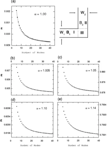
By using the mode matching technique, we are able to obtain the bound state energy of an electron in the quantum dot formed at the intersection of the arms of a L-shaped or a T-shaped quantum wire when magnetic fields are applied on the arms. In order to make the numerical computation be-come feasible, the numbers of modes in the wider arms are properly considered while the ratios of arm widths is nearly zero or extremely large. Moreover, different number of modes for each arm is also carefully considered. To make sure whether our numerical calculation is reliable or not, the tendency of convergence for different number of modes in-cluded in our calculation is presented in Fig. 2 for an LQW with some typical ␣ values. Figure 2共a兲 presents the result for the symmetric case, i.e., ␣⫽1 or W₂⫽W₁. And Figs. 2共b兲, 2共c兲, 2共d兲, and 2共e兲 are the obtained results for cases of

␣⫽1.005,␣⫽1.05,␣⫽1.10, and␣⫽1.14, respectively. The tendency of convergence for different number of modes in-cluded in our calculation for TQW system is shown in Fig. 3. As shown in Fig. 3共a兲, three cases are presented: solid down-triangle represents the result obtained by using ␣⫽1 共i.e.,

W2⫽W1兲, solid circle presents the result for ␣⫽1.01, and

solid up-triangle for ␣⫽1.05. Fig. 3共b兲 and 共c兲 present the results obtained for␣⫽1.10 and␣⫽1.33, respectively. It is noticeable that our calculations converge rapidly even in the

case with large value of ␣ though we just included same number of modes in each region. Our results agree well with previous works.24 –27

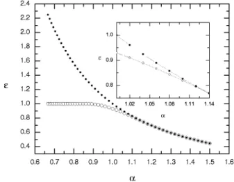
B. The bound states in QDs at zero field

Figure 4 presents the variation of the calculated bound state energies of an electron in a LQW as a function of arm ratio ␣. For clarity, the bound state energy of the electron is expressed in terms of the dimensionless quantity ⑀⫽E/E₁ throughout this article, where E₁⫽(ប2_␲2_/2m_*_W

1

2_{) is the}

first subband level in arm 1共region 1兲. One can note from the figure that the bound state energy of the electron becomes smaller as the arm ratio ␣ becomes larger. For ␣⫽1 共i.e.,

W₁⫽W₂兲, i.e., a symmetric L-shaped quantum wire, we have rm⫽tmat zero magnetic field, the bound state energy of the

electron is obtained as 0.92964E1. For asymmetric

geom-etries, the calculated bound state energy ⑀ goes down and behaves like the curve of 1/␣2 as the asymmetric parameter

␣is increased larger than 1.14. A deviation from the curve of 1/␣2 is observed in the region of␣⭐1.14 as can be seen in the inset of Fig. 4. The result can be ascribed to the fact that the bound state energy of the electron matches the subband energy of arm 2 due to the lateral confinement of region II.

FIG. 2. The convergence tests of the number of modes for LQW system for different␣.共a兲␣⫽1.00, 共b兲␣⫽1.005, 共c兲␣⫽1.01, 共d兲␣⫽1.05, and 共e兲

␣⫽1.14. Even for large␣⫽1.14, our calculation converges rapidly. FIG. 3. The convergence tests of the number of modes for T-shaped QW_{system for}_{共a兲 solid down-triangle for}_␣_{⫽1.00, solid circle for}_␣_{⫽1.01, and}

solid up-triangle for ␣⫽1.05, 共b兲 open up-triangle for ␣⫽1.10, 共c兲 open square for␣⫽1.33. Even for large␣⫽1.33, our calculation converges rap-idly.

3057

(6)

Since in this circumstance, 1/␣2(␲/W1)2 is just equal to

(␲/W2)2, which is the first subband level of the vertical

wire. As the width W2becomes larger and larger, this energy

level becomes lower and lower, and gradually coincides with the bound state energy level of the electron. Thus the elec-tron is unable to be bounded in the corner region any more. This can be understood by the clue exhibited in the distribu-tion of the probability density of the electrons. The probabil-ity densprobabil-ity of electrons in the LQW can be evaluated by summing up over all terms

␳共x,y兲⫽

兺

n_⫽1 N

兩⌿n共x,y兲兩2. 共15兲

Figure 5 shows the contour plots of the probability den-sity distribution of the bound states for several␣values in an asymmetric LQW system. The distributions are normalized to their own maxima for simplicity, and the most inner con-tour curve possesses the highest probability density. In the

case of␣⫽1, the contour of the probability density distribu-tion reflects a mirror symmetry due to its symmetric geom-etry as can be seen from Fig. 5共a兲. The electron piles up at the corner region as the localized state is formed. In these cases, the probability density distribution decays exponen-tially in the arm regions, such that the electron is unable to go far away from the corner. One can also note from Fig. 5, as the structure asymmetry of the LQW becomes prominent, e.g., as ␣ increases from 1.005 in 共b兲 to 1.05 in 共c兲 and finally 1.10 in共d兲, the probability density distribution gradu-ally extends to the wider arm region. As the asymmetry be-comes more obviously, the peak of the electron probability density distribution transmits eventually out of the corner region providing the electronic energy is larger than the bot-tom of the subband of the wider arm. However, if the energy of the electron state is less than or just equal to the subband bottom, the electron is still bounded inside the corner and does not move to the right or to the left. Therefore, this state cannot transmit in the arm and does not contribute to the conductance. Hence, it consequently results in valleys or dips near the transmission thresholds.17

Now let us consider the case of a TQW. For a TQW, if we change the ratio␣⫽W2/W1, we do not change its image

symmetry. Thus, it can be expected that at least one bound state can exist in TQW no matter how large the width of the transverse arm is. Figure 6 shows the bound state energy of the electron in a TQW as a function of␣. One can see from the figure that bound state energy approaches unity as the width of the vertical arm becomes very small, and behaves like a curve of 1/␣2while the value␣becomes larger. This is similar to the case of a LQW. The reason of this result can be understood intuitively that the wave function of the electron is purged out of the vertical arm when it becomes very nar-row and thus the wave function is almost squeezed inside the longitudinal arm, therefore, the energy of this state is close to the first threshold energy E1 of the horizontal arm with a

width of W1. This bound state of the electron exists as long

FIG. 4. The bound state energy⑀vs the asymmetric ratio␣⫽W2/W1 at

zero magnetic field strength. Open circle is our result. The dotted line is the curve of 1/␣as a guide to eyes. E1⫽(ប2␲2)/(2m*W1

2

) is the first threshold energy of arm 1共the region I兲.

FIG. 5. The probability density distributions of electron in LQW for differ-ent asymmetric parameter␣.共a兲 ␣⫽1, 共b兲␣⫽1.005, 共c兲␣⫽1.01, 共d兲␣

⫽1.05, and 共e兲 ␣⫽1.1. All distributions are normalized to its maximum

value for simplicity.

FIG. 6. The bound state energy ⑀ of a TQW plotted in unit of E1 as a

function of␣. The bound state energy of the electron approaches to unity for

␣Ⰶ1 and can be approximately expressed by the curve 1/␣2_for_␣_⭓1.33

(7)

as the vertical arm is infinite long, and is expected to disap-pear owing to the effect of leakage if the arms is finite in length.

Actually, the bound state energies of electrons of the QDs are slightly higher than 1/␣2 for large ␣, and also slightly lower than 1 for small ␣. The bound state of the electron thus always exists no matter how large the ratio␣is, except for one of the arms has finite length. One can observe this result from the contour plots of the probabilities depicted in Fig. 7 for ␣⭓1 and Fig. 8 for␣⬍1.

It often involves anisotropic factors in semiconductor systems. The anisotropic Hamiltonian for an anisotropic heavy hole at zero field is given by

Hˆ⫽⫺

冋

ប 2 2mx* ⳵2 ⳵x2⫹ ប2 2my* ⳵2 ⳵y2

册

⫹V共x,y兲. 共16兲

Let y˜⫽(m_y*/m_x*)1/2_{y , then Eq.}_{共16兲 can be rewritten as}

Hˆ⫽⫺ ប 2 2m_x*

冋

⳵2 ⳵x2⫹ ⳵2 ⳵˜y2

册

⫹V共x,y˜兲. 共17兲

Comparing with Eqs. 共7兲 and 共8兲, we have the same Schro¨-dinger equations if we change the variable y into y˜ . The

anisotropic factor ␣⫽(m_y*/m_x*)1/2 is large as 1.348 for a typical GaAs system if we adapt the values: mhh关110兴 ⫽0.69m0 and mhh关001兴⫽0.38m0.5 This value gives rise to

the result that the hole is extremely anisotropic distributed in TQW structure. However, it should be still bounded as we already mentioned.

C. Effects of magnetic fields on the electronic bound state in a QD

For simplicity and clarity, the QDs are considered to be formed on symmetric two-dimensional LQW and TQW sys-tems, that is only the case of W2⫽W1. The calculated bound

state energies of the electrons in the QD formed in LQWs under the magnetic fields are plotted as functions of the field strength f⫽ប␻c/E1, as depicted in Fig. 9共a兲 for case of both

arms and in Fig. 9共b兲 for case of only one arm in the LQW system subjected to magnetic field, where ␻c is cyclotron

frequency of the electron. One can observe that the bound state always exists when the magnetic field is applied to both arms. The energy level of the electron in this case is mono-tonically increased while the magnetic field is increased. In the contrast, curve共b兲 shows the energy of the bound state of the electron is pushed up by the applied magnetic field, and then it goes up to E₁. Thus, the electron can escape via the field free arm.

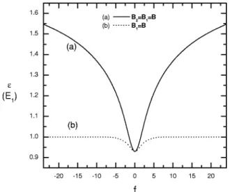
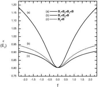
For the symmetric TQW, there are two main configura-tions of the applicaconfigura-tions of magnetic fields. The case of sym-metrically applying magnetic fields to the system includes three types which are shown in Fig. 10. In Fig. 10, curve共a兲 displays the confinement energy versus the field strength when all arms are acted by the same magnetic field B, curve 共b兲 displays the energy versus the field strength when the two horizontal arms are acted by the same magnetic field, and curve 共c兲 displays that only the vertical arm is acted by the magnetic field. The same quadratic dependence of magnetic

FIG. 7. The contour plots of the relative probability of the bound state of an electron in an asymmetric TQW.

FIG. 8. The contour plots of the relative probability of the electron bound state in an asymmetric TQW.

FIG. 9. The bound state energy⑀vs the field strength f.共a兲 For both arms being acted by the magnetic fields in LQW system.共b兲 For only one arm being acted by the magnetic fields. The dimensionless field strength f is normalized by E1.

3059

(8)

field of the bound state energy of the electron is revealed again for the weak field strength, and the linear dependence appears in the strong field region as the case of LQW. For these symmetric configurations of magnetic field, the bound state always exists. It is found that the more arms are acted by the magnetic field, the higher energy of the bound state of the electron is obtained due to the stronger depletion effect. The quadratic dependence region is wider if the depletion effect is smaller, as shown in curves共a兲, 共b兲, and 共c兲 of Fig. 10. Obviously, the bound state level of the electron in a TQW system locates deeper than that in a LQW, that is, the TQW system has a weaker confinement potential than the LQW system. This causes a deviation of bound energies about 0.12E1. We also calculated several relative probability

con-tours of the bound state of the electron under the magnetic fields as displayed in Fig. 11.

For the case of inhomogeneous magnetic field applying on the TQW, the energy levels of electron are shown in curves 共a兲 and 共b兲 of Fig. 12. Curve 共a兲 of Fig. 12 presents

the case of the magnetic fields applying to region I共or region II兲 and region III of the TQW system, and curve 共b兲 of Fig. 12 presents that of the magnetic field applying to region I共or region II兲 only. These curves consist of the former result that the more regions are acted by magnetic fields, the higher energy of the bound state of the electron are obtained. And from Fig. 12共a兲, it can be observed that the energy of the bound state approaches E1 for a higher magnetic strength.

This is a similar consequence of the conclusion obtained in the LQW system. The behavior is also found from curve共b兲 of Fig. 12, however, its value approaches the energy of the QD in a symmetric LQW system. Both curves共a兲 and 共b兲 of Fig. 12 show quadratic feature for weaker magnetic field regions due to the depletion effect of magnetic field. Com-pare curves共a兲 and 共b兲 of Fig. 12, one can notice that a wider quadratic region directly reflects the weaker depletion effect of the magnetic fields.

The external perpendicular magnetic fields introduce a depleting effect on electrons and add an extra potential sur-rounding the QD. From Eqs. 共7兲, 共8兲, and 共9兲, one can ob-serve that the effective potentials introduced by the magnetic fields are k dependent. For the bound state, these effective potentials are complex due to the pure imaginary兵k其. There-fore, one cannot easily figure out the effective potentials.

One can expect intuitively that the magnetic field adds the lowest Landau level ប␻c/2⫽បeB/2m* directly to the

quantum dot system共in the corner region兲 an extra potential. Such levels are added into the wire regions surrounding the QD. However, the field plays another role due to the essen-tial physics of the magnetism. Qualitatively, one can under-stand the effect induced by the magnetic field on the bound state of the electron by considering an one-dimensional shal-low quantum well with finite height U0. In the limit of

shal-low well, there is only one bound state exists in the well. Its level energy is given by E0⫽U0⫺(m*W2/2ប2)U0

2

,28which

FIG. 10. The bound state energy⑀of T-shaped QW as a function of the field strength f. Curve共a兲 for all arms being acted by magnetic fields. The field strength f is normalized by E1. Curve共b兲 for the horizontal arms being

acted by magnetic fields, and curve共c兲 for only vertical arm being acted by magnetic field. The dimensionless field strength f is normalized by E1.

FIG. 11. The contour plots of the relative probability of the electron bound state in TQW under the magnetic field.

FIG. 12. The bound state energy⑀of T-shaped QW as a function of the field strength f. Curve共a兲 for the region I 共or region II兲 and region III being acted by the same magnetic field. Curve共b兲 for only region I 共or region II兲 being acted by magnetic field. The dimensionless field strength f is normalized by E1.

(9)

is near the top of the well. Let us consider that if the poten-tial height is changed to U₀⫹1/2ប␻_cdue to the application of the external magnetic field, then how does the bound state energy of the electron change? This is not quite intuitive to figure out. First, it is easy to see that the variation of the state level depends linearly on the potential height, i.e.,

⳵E0

⳵U₀⫽1⫺ m*W2

ប2 U0. 共18兲

To take into account the depletion effect of the magnetic field, which effectively suppress the envelop of the electron wave, the variation of the state level is assumed as

⳵E0

⳵W⫽⫺ m*W

ប2 U0

2_. _共19兲

Obviously, once we need to take the well shrunk into ac-count, the quadratic form of the dependence of magnetic field has to be considered also. This remarkable simple model manifests the essential important effect of geometric scale in quantum behavior, and also manifests one of the essential properties of magnetism at the same time. However, in the strong magnetic field strength region, the shrinking of the geometric scale is no longer prominent, because the elec-tron wave function is squeezed to a certain local area. And there is fewer probability left in the arms, therefore there is less influence of the magnetic field on the electron. Thus, the energy of bound state of the electron depends simply on the added effective potential, such that it seems likely to depend linearly on the magnetic field in the high field strength re-gion.

IV. SUMMARY

The asymmetry parameter, which is defined as ␣ ⫽W2/W1, plays an important role in the formation of a QD.

The asymmetry parameter strongly affects the bound state of an electron in a QD. When the asymmetry parameter ␣ in-creases, the bound state energy of the electron is lower as expected. On the other hand, when the applied magnetic field increases, the bound state level of the electron is pushed higher and higher and the electron begins to be unbounded if there is an arm with finite length which offers a passway for electron to leak out. Generally, the bound state level of an electron in the QD formed in a TQW system is lower than that in LQW system. This fact reflects the weaker confine-ment of the geometry. It is found that the magnetic field also affects the bound state, even though the spin of the electron is not taken into account. Parabolic dependence of the bound state energy of the electron in weak field region on the field strength is understood as a result of the depletion effect. In the contrast, linear dependence in high field region is found to be resulted from the additional effective potential due to the magnetic field.

ACKNOWLEDGMENT

This work is supported partially by National Science Council, Taiwan under the Grant No. NSC90-2112-M-009-018.

1

Y.-C. Chang, L. L. Chang, and L. Esaki, Appl. Phys. Lett. 47, 1324

共1985兲.

2

F. Sols, M. Macucci, U. Ravaili, and K. Hess, J. Appl. Phys. 66, 3892

共1989兲; F. Sols and M. Macucci, Phys. Rev. B 41, 11887 共1990兲.

3

D. S. Chuu, C. M. Hsiao, and W. N. Mei, Phys. Rev. B 46, 3898共1992兲; C. M. Hsiao, W. N. Mei, and D. S. Chuu, Solid State Commun. 81, 807

共1992兲.

4_{S. N. Walck, T. L. Reinecke, and P. A. Knipp, Phys. Rev. B 56, 9235}

共1997兲.

5_{S. Glutsch, F. Bechstedt, W. Wegscheider, and G. Schedekbeck, Phys. Rev.}

B 56, 4108共1997兲.

6_{W. Langbein, H. Gislason, and J. M. Hvam, Phys. Rev. B 54, 14595}

共1996兲.

7_{H. Gislason, C. B. So}_{”rensen, and J. M. Hvam, Appl. Phys. Lett. 69, 800}

共1996兲.

8_{H. Gislason, W. Langbein, and J. M. Hvam, Appl. Phys. Lett. 69, 3248}

共1996兲.

9_{T. Someya, H. Akiyama, and H. Sakaki, Phys. Rev. Lett. 74, 3664}_共1995兲;

T. Someya, H. Akiyama, and H. Sakaki, Appl. Phys. Lett. 66, 3672共1995兲.

10

A. Yacoby, H. L. Stormer, N. S. Wingreen, L. N. Pfeiffre, K. W. Baldwin, and K. W. West, Phys. Rev. Lett. 77, 4612共1996兲.

11

R. Sˇordan and K. Nikolic´, Appl. Phys. Lett. 68, 3599共1996兲.

12_{L. Burgnies, O. Vanbe´sien, and D. Lippens, Appl. Phys. Lett. 71, 803}

共1997兲.

13_{G. Goldoni, F. Rossi, and E. Molinari, Appl. Phys. Lett. 71, 1519}_共1997兲; 69, 2965 共1996兲; G. Golodoni, F. Rossi, E. Molinari, and A. Fasolino, Phys. Rev. B 55, 7110共1997兲; F. Rossi, G. Goldoni, and E. Molinari, Phys. Rev. Lett. 78, 3527共1997兲.

14_{M. Yoshita, H. Akiyama, T. Someya, and H. Sakaki, J. Appl. Phys. 83,}

3777共1998兲; T. Someya, H. Akiyama, and H. Sakaki, Phys. Rev. Lett. 76, 2965共1996兲; H. Akiyama, T. Someya, M. Yoshita, T. Sakai, and H. Sasaki, Phys. Rev. B 57, 3765共1998兲.

15_{D. Brinkmann and G. Fishman, Phys. Rev. B 56, 15211}_共1997兲. 16

J. L. Bohn, Phys. Rev. B 56, 4132共1997兲.

17_{B.-Y. Gu, Y. K. Lin, and D. S. Chuu, J. Appl. Phys. 86, 1013}_{共1999兲; K.-Q.}

Chen, B.-Y. Gu, Y. K. Lin, and D. S. Chuu, Int. J. Mod. Phys. B 13, 903

共1999兲.

18_{M. Grundmann, O. Stier, and D. Bimberg, Phys. Rev. B 58, 10557}_共1998兲. 19_{C.-T. Liang, I. M. Castleton, J. E. F. Frost, C. H. W. Barnes, C. G. Smith,}

C. J. B. Ford, D. A. Ritchie, and M. Pepper, Phys. Rev. B 55, 6723共1997兲.

20_{C.-T. Liang, M. Y. Simmons, C. G. Smith, G. H. Kim, D. A. Ritchie, and}

M. Pepper, Phys. Rev. Lett. 81, 3507共1998兲.

21

L. Solimany and B. Kramer, Solid State Commun. 96, 471共1995兲.

22_{H.-S. Sim, K.-H. Ahn, K.-J. Chang, G. Ihm, N. Kim, and S.-J. Lee, Phys.}

Rev. Lett. 80, 1501共1998兲.

23

G. W. Bryant and Y. B. Band, Phys. Rev. B 63, 115304共2001兲.

24_{R. L. Schult, D. G. Ravenhall, and H. W. Wyld, Phys. Rev. B 39, 5476}

共1989兲.

25_{J. P. Carini, J. T. Londergan, K. Mullen, and D. P. Murdock, Phys. Rev. B} 46, 15538共1992兲; 48, 4503 共1993兲.