Received July 27, 1998; accepted November 29, 1999. Communicated by Chyi-Nan Chen.
243
Design Issues for Optimistic Distributed Discrete
Event Simulation
YI-BING LIN
Department of Computer Science and Information Engineering National Chiao Tung University
Hsinchu, Taiwan 300, R.O.C. E-mail: liny@csie.nctu.edu.tw
Simulation is a powerful tool for studying the dynamics of a system. However, simulation is time-consuming. Thus, it is natural to attempt to use multiple proces-sors to speed up the simulation process. Many protocols have been proposed to perform discrete event simulation in multi-processor environments. Most of these distributed discrete event simulation protocols are either conservative or optimistic. The most common optimistic distributed simulation protocol is called Time Warp. Several issues must be considered when designing a Time Warp simulation; examples are reducing the state saving overhead and designing the global control mechanism (i. e., global virtual time computation, memory management, distributed termination, and fault tolerance). This paper addresses these issues. We propose a heuristic to select the checkpoint interval to reduce the state saving overhead, generalize a previously proposed global virtual time computation algorithm, and present new algorithms for memory management, distributed termination, and fault tolerance. The main contribution of this paper is to provide guidelines for designing an efficient Time Warp simulation.
Keywords: discrete event simulation, distributed systems, fault tolerance, memory management, time warp
1. INTRODUCTION
A discrete event simulation consists of a series of events, along with times when they occur. Execution of any event can give rise to any number of events with later timestamps. All of this is straightforward in implementation if there is a centralized system with one event queue: we just execute the earliest not-yet-executed event next.
Since simulation is time-consuming, it is natural to attempt to use multiple processors to speed up the simulation process. In distributed discrete event simulation (or distributed
simulation), the simulated system is partitioned into a set of sub-systems that are simulated
by a set of processes that communicate by sending/receiving timestamped messages. The scheduling of an event for a sub-system at time t is simulated by sending a message with timestamp t to the corresponding process. The global event list and global clock of a sequential simulation do not exist in the distributed counterpart. Each process has its own input message queue and local clock. To correctly simulate a sub-system, the corresponding process must execute arriving messages in their timestamp order, as opposed to their real-time arrival order. To satisfy this causality constraint, a synchronization mechanism is
required. One of the most common synchronization protocols for distributed simulation is called Time Warp [12] (Different approaches to distributed simulation are discussed else-where [8, 15, 19, 22, 28, 31, 32].)
The Time Warp protocol takes an optimistic approach in which a process executes every message1 as soon as it arrives. If a message with an earlier timestamp subsequently
arrives (called a straggler), the process must roll back its state to the time of the straggler and re-execute from that point. To support rollback, several data structures are maintained in a process:
∑ Input queue: the set of all messages which have recently arrived. These messages
are sorted in their timestamp order. Some of them may have been processed.
∑ Local clock: the timestamp of the message being processed. If all the messages in
the input queue have been processed, then the local clock is set to •.
∑ Output queue: the set of negative copies (i.e., antimessages) of the positive
mes-sages the process has recently sent. An antimessage of a message m is exactly like
m in format and content except in one field: its sign. Two messages that are identical
except for opposite signs are said to be antimessages of one another.
∑ State queue: copies of the process’s recent states.
When a message arrives at a process pi with a timestamp no less than the local clock, it is inserted in the input queue. Process pi executes messages in the input queue in their timestamp order. Let ts(m) be the timestamp of a message m. Suppose that the scheduling of a message m is due to the execution of another message m0. Then the send time of m
(denoted as ts'(m)) is defined as the timestamp of m0. In other words, ts'(m) = ts(m0). Since the
execution of an event always schedules events with later timestamps, we have ts'(m) = ts(m0)
< ts(m). When m is executed, the following steps are performed: (i) The local clock advances to ts(m). (ii) Message m is processed. If any message m' is scheduled to another process pj during the execution, the antimessage of m' is also created. The positive message is sent to
pj, and the negative copy is inserted in the output queue in send time order. (iii) The new process state after the execution is added in the state queue. (Step (iii) is not necessarily performed for every event execution. However, the state of the process must be saved regularly.)
If a straggler subsequently arrives, the process must roll back its state to the time of the straggler and re-execute from that point. Consider the example shown in Fig. 1. A horizontal line represents the progress of a process in simulation time, and a dashed arrow represents sending a message. When pi’s local clock is b, it receives a message m with timestamp b' < b. Thus, pi is rolled back to the timestamp b'. During the roll back computation,
pi may have sent messages to other processes (cf. message f in Fig. 1). These output messages are potentially false messages because their timestamps are greater than the local clock. (A false message does not exist in the sequential simulation. That is, the message does not have any effect on the simulation and must be cancelled if it is created in Time Warp simulation.) The cancellation of a potential false message f sent from pi to pj is done by sending the corresponding negative message f (which is stored in the output queue of pi 1A message consists of six fields: send time, timestamp (or receive time), sender, receiver, sign, and text. We will elaborate on these fields later.
when f is sent). Once pj receives f , it discards f and any effect caused by f. One may assume that all output messages f generated during the roll back computation are false, and negative messages f are immediately sent to cancel these output messages at the time the rollback occurs. This is called aggressive cancellation. On the other hand, one may assume that all messages sent during the roll back computation are true (i.e., not false), and are not cancelled at the time the rollback occurs. After the rollback, new messages m1, m2, ... will be generated.
Negative messages f need only be sent for potential false messages that are not regener-ated (i.e., f π mi). Depending on the application, lazy cancellation may outperform aggressive cancellation or vice versa. Guidelines for designing the rollback mechanism can be found elsewhere [21, 30].
2 In some studies [8, 18], the timestamps of unprocessed messages are considered in computing GVT, instead of their send times. This paper follows the original definition of GVT given by Jefferson [12].
Besides the rollback (local control) mechanism, a global control mechanism for Time Warp is required. The central concept of the global control mechanism is global virtual time (GVT). Let an unprocessed message be a message in the input queue of a process that has not yet been executed. GVT is defined as follows.
Definition 1: GVT at time t (denoted as GVT(t)) is the minimum of (i) the values of all local
clocks at time t, (ii) the timestamps of all unprocessed messages, and (iii) the send times2 of
all transient messages.
At any real time, there exists a global virtual time GVT such that all executed messages with timestamps earlier than GVT will not be rolled back. Based on GVT, the global control mechanism addresses several critical issues, such as garbage collection, distributed termination, and fault tolerance.
This paper concentrates on reducing the state saving overhead and the design issues for the Time Warp global control mechanism. The paper is organized as follows. Section 2 derives a heuristic used to select the checkpoint interval to reduce the state saving overhead. Section 3 generalizes a previously proposed GVT computation algorithm. Sections 4-6 present new algorithms for memory management, distributed termination, and fault tolerance.
Fig.1. Effect of Rollback. A horizontal line represents the progress of a process in simulation time, and a dashed arrow represents sending a message.
2. REDUCING THE STATE SAVING OVERHEAD
In a Time Warp simulation, the state of each process must be saved regularly (regardless of whether or not rollbacks actually occur). Lin and Lazowska [20] have indicated that the performance of Time Warp is dominated by the efficiency of state saving. Thus, it is impor-tant to reduce the state saving overhead.
There are two approaches to reducing the state saving overhead. One approach is to accelerate the state saving process. Fujimoto et al. [9] developed special-purpose hardware to support fast state saving. A complementary approach is to reduce the frequency of state saving. This section pursues the second approach. We give a heuristic to select the checkpoint interval to reduce the state saving overhead and report on the confirmation of our results in an experimental study conducted by Preiss et al. [29].
From a model similar to that in [11, 35, 37], we derive bounds for the optimal checkpoint interval nopt. Note that our derivations are based on several simplifying assumptions. Thus, the term “optimal” means the best possible choice of the parameter nopt, subject to our assumptions.
Consider a process p in a Time Warp simulation. We assume that there is no message preemption, and that a state saving operation occurs atomically with the completion of the checkpointed event. We refer to the interval between two consecutive rollbacks of p as a
computation cycle. Suppose every n message executions are followed by a state saving
event (i.e., the execution of the nth event is checkpointed). n is called the checkpoint
interval. Consider the ith computation cycle of length Rn,i as shown in Fig.2.
In this figure, a solid circle represents a state saving event. After Rn,i events have been executed, a straggler arrives, which undoes bn,i events. However, it is necessary to roll back to the first checkpoint (but not include the checkpoint itself) prior to the timestamp of the straggler, and an extra gn,i event must be re-executed to restore the current process state. For convenience of analysis, the executions of these events are assumed to be in the i + 1st computation cycle. A computation cycle i consists of three parts:
∑ rollback and restoring the current process state by re-executing Ln,i-1 events (cf. Fig. 2),
∑ forward executions (the executions of an,i events in Fig. 2),
∑ and periodic checkpointing (cf. the solid circles in Fig. 2).
Fig. 2. The ith computation cycle.
Thus, Rx,i can be expressed as
Note that an,i may be negative (i.e., a straggler message arrives before all Ln,i-1 mes-sages have been executed), but an,i + Ln,i-1 is always positive. In our model, the state saving overhead Dn,i for the ith computation cycle is defined as the overhead needed to re-execute the Ln,i-1 events in the previous computation cycle plus the overhead of the state saving operations done among Ln,i-1 + an,i events. Let Ns be the overhead of saving a process state, assumed to be a constant. Let Ni,j be the execution time of the jth event (j £ Rn,i) in the ith computation cycle. Assume that the process state is checkpointed before the first event is executed, then the state saving overhead, Dn,i, of the ith computation cycle is
∆χ χ χ χ γ δ α χ δ α γ χ δ χ , , , , , , , . , i i j i s i i s j i i = + = + ∑ − = − 1 1 1 1 otherwise (2)
Equation (2) consists of two components. The first component represents the over-head for restoring the current process state (when i = 1, Ln,i-1 = 0 and the component does not exist). The second component represents the overhead for periodic checkpointing. This equation holds whether an,i³ bn,i or an,i < bn,i (an,1³ bn,1, according to the definition of a Time Warp simulation). Let kn be the number of rollbacks that occur in a process when the checkpoint interval is n. Let ∆χ ∆χ
χ = ∑ = E i i k , . 1
Then Dn can be expressed as ∆χ =∆Cχ+∆Uχ,
where ∆Cχ
is the time devoted to periodic checkpointing that ∆Uχ
is the time devoted to re-executing the extra undone events needed to restore the current process state. Our goal is to choose an optimal n value which minimizes the net effect Dn. We first derive a lower bound
∆x
− and an upper bound ∆ χ + for D
n with a fixed checkpoint interval. Let Cn be the number of checkpoints required in a process. From (2),
C i i i k χ χ χ χ α χ α χγ χ = + + ∑ − = ,1 , , 1 2 .
Assume that the behavior of the system is not affected by the checkpoint interval; that is, for all n, the process states are the same at the end of a computation cycle. This assumption is reasonable when the system being simulated is homogeneous. However, it does not reflect the real world in general. Thus, our solution should be considered as a heuristic for checkpoint interval selection. From this assumption, we have
kn = k1 = k, and for all i an,i = a1,i = ai and bn,i = b1,i = bi. (3) Let Nn be the number of events (including the roll back events) executed in a process when the checkpoint interval is n. Since L1,i = 0, (1) and (3) imply that an,i > 0, and
N N x j j k χ = + ∑γ = 1 1 , . (4)
It is not possible to derive Dn without knowing the distributions of ai and bi. Lacking knowledge of these distributions, we will instead derive bounds for Dn.
To derive a lower bound for Dn, consider the ith computation cycle in Fig. 2. Execution of every n events requires a checkpoint, except for the last γ′χ,i events. (The process is checkpointed at the beginning; then, every n event executions are followed by a checkpointing operation.) In other words, the execution of the last γ′χ,i events does not incur checkpointing overhead. Thus, the best case occurs when γ′ = −χ,i χ 1. Then, Cn is bounded below as
Cχ ≥ Nχ−(χχ−1)k = Nχχ+k−k. (5)
If we assume that Ln,i is uniformly distributed in [0, n - 1], then a tighter bound can be obtained. Let α = Nk1, and let d be the expected event execution time. Then from (2), (4) and
(5), a lower bound ∆−χ for Dn is derived as follows:
∆ ∆ χ χ χ δ χ χ δ χ δ αχ δ ≥ − + + − + − = − + + − = − ( ) ( ) ( ) . 1 2 1 2 1 2 1 2 1 1 1 k N k k k k s s (6)
The checkpoint interval that minimizes (6) is
χ+= αδ+ δ (2 1) s (7) It is interesting to note that (7) is almost identical to Young’s result [37] under the proper interpretation of the parameters. To derive an upper bound for Dn, let γ′χ,i= 0 and Ln, i = n - 1. Then the number of checkpoints required in a process is bounded above by
Cχ ≤ Nχχ ≤ N1+(χχ−1)k. (8)
From (2) and (8), an upper bound ∆+χfor Dn is derived as: ∆ ∆ χ χ χ δ χχ δ χ δ α χχ δ ≤ − + + − = − + + − = + k N k k s s ( ) ( ) ( ) ( ) . 1 1 1 1 1 (9)
The checkpoint interval that minimizes (9) is
χ−= α−δ δ ( ) . 1 s
Fig. 3 plots the curves for ∆−χ and ∆+χ. The functions for both ∆+χ and ∆−χ are of the
Since f2(n) is a parabola, the effect of f1(n) makes f(n) decrease quickly as n increases
before the minimum is reached (in Fig. 3, the minima are ∆+min= ∆+χ− and ∆−min= ∆−χ+), and increase slowly as n increases after the minimum is reached. From Fig. 3, the optimal check-point interval nopt is bounded by M-£ nopt£ M+, where M- and M+ are the roots of the equation
∆−χ= ∆min
+ . Note that M - £ n -£ n +£ M + and M + - n +³ n + - M -, and
M+→χ+,M−→χ−, as ∆+χ+ →∆−χ. (10) Since the derivations for M- and M+ are more complicated than the derivations for n
-and n +, it is more practical to determine n
opt in terms of n - and n +. As indicated by (9), this is a good approximation when ∆+χ→∆−χ.
We make the following observations.
∑ If the execution times of events are random variables, then Dn is affected by the mean of the execution times but is insensitive to the distribution of the execution times. This is derived from the strong law of large numbers.
∑ For a fixed n, the state saving overhead Dn decreases as α increases. This implies that reducing the state saving overhead is important for simulation with small α.
∑ Erring on the side of a n value that is too large will degrade performance less than
erring on the side of a n value that is too small.
∑ A large n should be chosen if (i) δδs
is large, and/or (ii) α is large. Intuitively, if ds is small (compared with d), then ∆Cχ only has an insignificant contribution to Dn. Thus, a small n should be chosen to minimize ∆Uχ. For a large α, ∆Cχ has a more significant
effect on Dn than ∆Uχ does. Thus, a large n should be chosen to reduce ∆Cχ. When
α= • (i.e., no rollback occurs at process p), no state saving is required, and n = •
should be selected.
Preiss et al. [29] have conducted experiments to study our simple heuristic. In their experiments, the execution times of simulation were measured instead of the state saving overhead Dn. Interestingly, the curves for the execution times have the same shapes as do the curves in Fig. 3. The experiments show that for the round-robin processor scheduling
policy 3 and for both aggressive cancellation and lazy cancellation, the optimal checkpoint
intervals fall in the interval [n -, n +] or are slightly higher. For the smallest timestamp first
policy, 4 the optimal checkpoint intervals are larger than n +. Although M + was not known in
the experiments, we believe that the optimal checkpoint intervals all fall in [n +, M +]. The
experiments also indicated that Dn1QDn2 for n1, n2Π[n +, nopt]. Thus, this experimental study concluded that n + is a good predictor for the optimal checkpoint interval. We note that in
these experiments, the parameters α, ds and d were obtained after the simulation run finished. A large issue is the fact that these parameters are seldom known ahead of time and are a function of the application characteristics. One way to obtain the values for the parameters is to compute these parameters during the simulation and update the values dynamically. Several issues about the use of our simple heuristic for reducing the state saving overhead are being investigated at the Jet Propulsion Laboratory [2, 33]. Bellenot’s experiments indi-cated that our heuristic is less accurate as the number of processors available increases. The reason is simple. The derivation of our heuristic assumes that processors are not idle during the simulation. (This assumption is generally true when the simulated system is large.) As the number of processors increases, the number of idle processors also increases, which may invalidate our assumption. Thus, we conclude that the heuristic is useful when the size of the simulated system is large.
3. GLOBAL VIRTUAL TIME COMPUTATION
Time Warp requires a global control mechanism to address several critical problems such as memory management, distributed termination and fault tolerance. The central con-cept behind the global control mechanism is based on GVT. Since GVT is smaller than the timestamp of every unprocessed message in the system, we have the following theorem.
Theorem 1 [12]: At time t, no event with a timestamp earlier than GVT(t) can be rolled back,
and such events may be irrevocably committed with safety.
Jefferson [12] showed that GVT is a non-decreasing function of time, which guaran-tees global progress of the Time Warp simulation.
In a shared memory multiprocessor environment, GVT can be easily computed [7]. On the other hand, GVT cannot be easily obtained in a fully distributed environment where messages might not be delivered in the order they are sent. (In such an environment, the transient messages in the system cannot be directly accessed.) In most approaches [3, 18, 27, 34], the task of finding GVT involves all the processes in the system. One of the processes, called the coordinator, is assigned to initiate the task. The coordinator broad-casts a STARTGVT message to all processes. Then every process computes its local mini-mum (to be defined), and reports this value to the coordinator. When all the local minima are received, the coordinator computes the minimum among these local minima, and GVT is found.
3 In the round-robin policy, the processes that are ready to execute (i.e., the processes that have messages to process) are allowed to process messages in round-robin fashion one at a time.
4 In the smallest timestamp first policy [23] or the minimum message timestamp policy [29], a process with smaller timestamp event (i.e., the next event to be executed in the process has a smaller timestamp) has higher priority for execution.
In a GVT algorithm, control messages (such as STARTGVT) are sent to perform GVT computation. These messages are distinguished from data messages, the normal messages sent in Time Warp simulation. Most GVT algorithms are based on Samadi’s approach [34]. In this approach, when process q receives a data message from p, it needs to send an acknowledgement back to p. We have proposed a GVT algorithm [18] that does not require acknowledgements for data messages. Thus, this algorithm can eliminate about 50% of the message sending during the simulation. However, the algorithm assumes that the set of processes that send messages to a process is pre-defined. This section removes this restriction.
Consider a pair of processes p and q. A message has a sequence number i if it is the
ith message (denoted as mi) sent from a process p to a process q. Consider an example of a send time histogram of messages sent from p to q in the time interval [0, t] as shown in Fig. 4. Note that a message with a larger sequence number may have a smaller send time due to a rollback in p. Let a valley be a message mi such that i = 1 or ts'(mi) < ts'(mi-1), i > 2. (Thus,
m1 is always a valley.) In Fig. 4, the set of valleys is {m1, m21, m50, m72}. The message with the
smallest send time is among these valleys. Thus, to find the minimal send time of messages in transit, we only need to consider those valleys in transit.
To obtain the minimal timestamp of transient messages, a set Vp(q) is maintained in process p to record the send time information of valleys that have been sent from p to q. If we represent a valley m as a (sn, ts') pair, where sn and ts' are the sequence number and send time of m, respectively, then the set Vp(q) for the example in Fig. 4 is
Vp(q) = {(1,10), (21,30), (50,50), (72,20), (80,70)}.
When process p sends a message m to process p, it checks if m is a valley. If it is, Vp (q) is updated to reflect the sending of m.
In process q, a set SNq(p) is used to record the (sequence number) ranges of messages which are sent from p and have been received by q. An element (i.e., a range) in SNq(p) is of the form (snf, snl), where snf is the sequence number of the first message in the range, and snl is the sequence number of the last message in the range. We note that the sequence number holes in SNq(p) are due to the non-FIFO communication property in the distributed environment. If the messages received by q are those with sequence numbers 1, 2, ..., 20, 32, 33, ..., 67, 69, 70, ..., 108, and 120, 121, ..., 131, then
SNq(p) = {(1,20), (32,67), (69,108), (120,131)}.
When process q receives a message m from process p, SNq(p) is updated to reflect receipt of m.
Now, we will describe GVT computation. Consider a process p. Let the input set of p (denoted as SI(p)) be the set of processes that send messages to p, and let the output set of
p (denoted as SO(p)) be the set of processes that receive messages from p. Two types of
control messages (STARTGVT and TYPE1) are sent in the GVT computation. The coordina-tor p0 initiates GVT computation by broadcasting a message STARTGVT to every process.
When process p receives the message STARTGVT, it enters the following phase.
Phase 1. In this phase, p (i) computes lmp, the minimum of p’s local clock and the minimum
send times of all unprocessed messages in p’s input queue, and (ii) sends a message msg = (TYPE1, snq,p) to every process q Œ SI(p), where
snq p sn snfsnl SNq p l , ( ,min) ( ) = + ∈ 1
is the smallest sequence number of the transient message sent from q to p.
When p receives the first TYPE1 message from another process, it enters the following phase.
Phase 2. In this phase, p waits to receive a message msg = (TYPE1, snp,q) from every q ΠSO(p). Using snp,q, p locates the smallest send time bp,q of the transient messages from p to q by searching the set Vp(q). That is,
τp q sn ts Vpq sn snp q ts , ( , ) min( ), , . = ′ ′ ∈ ≥
After p has received all the TYPE1 messages, it computes τp τ q S p p q = ∈ min ( ) , 0 .
After p has completed both Phase 1 and Phase 2, it reports to the coordinator the local
minimum
LMp = min(lmp, bp).
After the coordinator has received all LMp, it computes
GVT LM
p p =
∀
The time when a process p enters Phase 1 may affect the correctness of the GVT computation. Suppose that process p enters Phase 1 at time tp. Due to the effect of rollback, if tpπ tq, it is possible that max
∀p LMp > GVT(tM), where tM=max∀p tp (i.e., (11) does not compute a lower bound for GVT). In Appendix A, we show that this problem is avoided if every process enters Phase 1 before Phase 2.
Theorem 2: Suppose that process p enters Phase 1 at time tp, and tM t
p p =
∀
max . If every process enters Phase 1 before Phase 2, then min
∀p LMp£ GVT(tM). Thus, the GVT algorithm for a process p is described as follows:
∑ If p receives the STARTGVT message before any TYPE1 message, it enters Phase 1. After p has sent all the TYPE1 messages, it enters Phase 2.
∑ If p receives any TYPE1 message msg before the STARTGVT message, then p enters Phase 1. After p completes Phase 1, it enters Phase 2 and processes msg. (In Phase 2, p ignores the arrival of the late message STARTGVT.)
In the above algorithm, the sets SI(p) and SO(p) are pre-defined. In a practical Time Warp simulation, both sets may change from time to time. To accommodate this situation, we assume that SI(p) and SO(p) are updated dynamically, i.e., SI(p) µ SI(p)»{q} (SO(p) µ SO(p)» {q}) when p receives (sends) the first data message from (to) q. With the dynamic input/ output sets, the algorithm just described may fail in the following scenario: Suppose that process q completes Phase 1 before it receives the first data message from p. Then p may expect to receive a TYPE1 message from q and never exit from Phase 2. This problem is solved by introducing a new control messages of type TYPE2: When p enters Phase 1, it also sends a TYPE2 message to every process q Œ SO(p). If (i) q has already completed Phase 1 when it receives a TYPE2 message from p, and if (ii) q did not send a TYPE1 message to p during Phase 1, then q sends msg = (TYPE1, 0) to p. (The message msg tells p that q did not receive any message from p when q entered Phase 1.) Thus, the complete algorithm is described as follows.
A process p enters the GVT computation mode when it receives the first message msg of type STARTGVT, TYPE1 or TYPE2. Upon receipt of msg, the following procedure is executed:
LMp = lmp, SGVT,I(p) = SI(p), SGVT,O(p) = SO(p);
for all q ΠSGVT,I(p) do send a message (TYPE1, lmp, snq,p) to q;
for all q'ΠSGVT,O(p) do send a message (TYPE2) to q';
Then p enters (modified) Phase 2 and handles the message msg: If msg = (TYPE1, snp,q'), then compute bp,q' and
If msg = (TYPE2) is from q' œ SGVT,I(p), then p sends a message (TYPE1, 0) to q'. After
p has received all the TYPE1 messages from processes in SGVT,O, the value LMp is sent to p0.
(Note that p may continue to receive TYPE2 messages before it receives the computed GVT from p0). The input (output) set of a process p considered in the GVT computation is SGVT,I (p) (SGVT,O(p)), the input (output) set when p enters Phase 1. This is required because the local minimum of process p is computed at the time when it enters Phase 1.
4. MEMORY MANAGEMENT
A parallel simulation may consume much more storage than space a sequential simu-lation no matter which parallel simusimu-lation protocol is used [13, 24]. Since extra memory is required to store the histories of processes, memory management for Time Warp is more critical than that for conservative simulation protocols, such as the Chandy-Misra approach. Basically, there are two approaches to reducing the memory consumption of Time Warp: reducing the state saving frequency as described in section 2 and fossil collection. Fossil collection is described as follows. Jefferson showed that:
Theorem 3: Let b < GVT(t). After time t, the following objects in a process pi are obsolete and can be deleted:
∑ the messages with timestamps no later than b in the input queue;
∑ the copies of the process state with timestamps earlier than b except for the one with
the largest timestamp no later than b (where the timestamp of a process state x, denoted as ts(x), is the local clock of pi when its process state is x);
∑ the messages in the output queue with send times no later than b.
Based on Theorem 3, fossil collection reclaims obsolete objects after GVT is computed. The frequency of GVT computation is basically determined by fossil collection: If a low frequency is chosen, a process may exhaust memory before the next fossil collection is performed. On the other hand, a high frequency may result in heavy overhead of GVT computation and fossil collection, and thus reduce the progress of the simulation. Some Time Warp implementations [14] periodically perform fossil collection on at fixed time intervals. Unfortunately, even if we reduce the state saving frequency and perform fossil collec-tion frequently, Time Warp may still consume much more storage space than a sequential simulation. Thus, it is important to design a memory management algorithm for Time Warp such that the space complexity of Time Warp is O(Ms), where Ms is the amount of storage consumed in sequential simulation. (A memory management algorithm for parallel simulation is called optimal if the amount of memory consumed by the algorithm is of the same order as the corresponding sequential simulation.) Jefferson proposed the first optimal memory man-agement algorithm, called cancelback [13]. In this protocol, when the Time Warp simulation runs out of memory, objects (i.e., input messages, states, or output messages) with send times later than GVT are cancelled to make more room. The cancelled objects will be repro-duced later. This section proposes another optimal protocol, called the artificial rollback
computa-tions” if necessary, to obtain more free memory space. Since the mechanism for the artificial rollback protocol is the same as that for the rollback mechanism, this protocol can be easily implemented.
We first introduce a special type of rollback that does not exist in normal Time Warp execution.
Definition 2: Without receiving a straggler, a process p may (on purpose) roll back its
computation to a timestamp b (b ≥ GVT) earlier than its local clock. Process p is said to
artificially roll back to timestamp b.
We impose the restriction b ≥ GVT for two reasons. First, artificial rollback should have the same properties as normal rollback, and no process can normally roll back to b < GVT . Second, if fossil collection is performed at GVT, a process cannot be artificially rolled back to a simulation time earlier than GVT because the earlier parts of process histories may already have been discarded. We will show that artificial rollback does not affect the correctness of Time Warp:
Theorem 4: Let S be a Time Warp simulation consisting of n processes p1, p2, ..., pn. Let cki
be the local clock of pi. Repeat the same simulation except that process pi artificially rolls back to a timestamp b < cki at time t and re-executes. Then the new Time Warp simulation is equivalent to S.
Proof: Let Ss be the sequential counterpart of S. Consider another sequential simulation S's, which is identical to Ss except that a new process pn+1 is added. Process pn+1 does not communicate with other processes except that it schedules an event e with timestamp b to pi. When the event occurs, pi does nothing. Thus, Ss and S's are equivalent in terms of the behaviors of p1, ..., pn. Consider S', the Time Warp implementation of S's. From the above discussion, S' is the same as S if we ignore pn+1. Suppose that pn+1 sends a message (corresponding to the occurrence of event e) to pi at time 0, and that the message sending delay for that message is t. (Note that assuming arbitrary message sending delay does not affect the correctness of Time Warp.) In effect, this is the same as an artificial rollback to pi. Thus, artificial rollbacks do not change the results of a Time Warp simulation. o From Theorem 4, a process may roll back to an earlier simulation time b ≥ GVT, and the memory used in the rolled back computation can be reclaimed. Later on, the rolled back computation (if it is correct) will be re-executed, which will produce the same results as the original Time Warp simulation.
Consider a shared memory environment. It is easy to prove that if we compute GVT, perform fossil collection, and roll back all processes to GVT, then the amount of memory used in Time Warp is of the same order as the amount of memory used in the sequential counterpart at simulation time GVT (cf. Theorem 6 in section 6).
With the artificial rollback protocol, Time Warp is able to reduce the amount of memory space used in parallel simulation (while other simulation approaches, such as the Chandy-Misra protocol cannot). However, progress of the simulation may be degraded. The trade-off between time and space is still an open question.
5. DISTRIBUTED TERMINATION
In most Time Warp implementations, termination detection is handled in terms of GVT: When a process p has processed all messages in its input queue, its local clock is set to •.
When GVT reaches •, all the local clocks must be •, and no messages can be in transit.
Thus, GVT is computed periodically to see if the simulation terminates (i.e., if GVT = •). To efficiently detect distributed termination, we should compute GVT infrequently at the begin-ning of the simulation. As time passes, the frequency should increase. However, such a selection of frequency may conflict with the needs of fossil collection. To simplify the selection of the GVT computation frequency, an algorithm that automatically detects distrib-uted termination without GVT computation might be attractive.
The distributed termination (DT) problem is non-trivial because no process has com-plete knowledge of the global state. Many algorithms [5, 6, 16, 17, 26] have been designed to detect distributed termination. Most of these algorithms deliver the control messages (i.e., the messages sent for DT detection) in pre-defined paths. Thus, in the view of these DT detection algorithms, the processes are connected in some fashion. Some algorithms con-nect the processes as a ring [16]. Others organize the processes as a tree (either dynamically [17] or statically [36]). In general, the “logical topologies” used in these DT detection algorithms may not match physical processor connections. For example, it is not efficient to implement a ring algorithm on a tree architecture, or vice versa. Even if the algorithm and the architecture match initially, inefficiency may be caused by process migration.
In this section, we propose a simple DT detection algorithm. In this algorithm, every process reports its termination to a coordinator which announces the termination of distribution. In other words, we have a “star” logical topology, and the shortest path is always chosen to deliver control messages between a process and the coordinator. One may argue that the coordinator may become a bottleneck. In Time Warp simulation, we expect that the number of control messages sent in DT detection is small compared with the number of data messages sent. Thus, if we have a dedicated coordinator process for DT detection, it will not be a bottleneck.
The sets Vp(q) and SNp(q) described in section 3 are used in our DT detection algorithm. This algorithm is based on the principle of message counting: If all processes are idle and the number of messages sent in the system is equal to the number of messages received, then the distributed computation has terminated.
Definition 3: Let SI(pi) be the input set of a process pi. Process pi satisfies the local
termina-tion conditermina-tion if and only if its local clock cki = •, and for all processes pj Œ SI(pi), |SNpi(pj)| = 1 (i.e., there is only one range in SNpi(pj)).
Note that if |SNpi(pj)| π 1, then at least one data message sent from pj to pi is in transit, and pi will be re-activated after the message is received. Let SNpi(pj) = {(snf, snl)}, and let ri,j = snl for all j Œ SI(pi) and si,k = Vpi(pk).sn for all k Œ SO(pi). If the local termination condition is satisfied, then ri,j (si,j) is the number of messages pi received from (sent to) pj. When this condition is detected, pi sends a message Mi = (IDLE, Si, Ri) to the coordinator p0, where
Si = {si,j|j ΠSO(pi)} and Ri = {ri,j|j ΠSI(pi)}.
The coordinator maintains two sets S' = {s'i,j| "i,j} and R' = {r'i,j|"i,j}. Initially, s'ij = r'i,j = 0 for all i,j. When p0 receives a message Mi = (IDLE, Si, Ri), the following code is executed to update S' (R' is updated in the similar way):
for all si,jΠSi do if si,j > s'i,j then s'i,j = si,j.
Now we will describe a distributed termination condition. When p0 satisfies this
condition, the distributed computation must have terminated.
Definition 4: Process p0 satisfies the distributed termination (DT) condition if and only if (i)
it receives at least one idle message from every process and (ii) s'i,j = r'j,i for all i,j. In Appendix B we prove the following theorem.
Theorem 5: The distributed computation terminates if the coordinator satisfies the DT
condition.
Thus, every time the coordinator p0 receives an IDLE message, it tests the DT condition.
If the condition is satisfied, then p0 announces distributed termination. It is apparent that
this algorithm is optimal in time complexity (if we ignore message contention): Suppose that a process pi is idle forever after time tpi. Let Dtpi be the message sending delay of the IDLE
message pi sends at time tpi. Then p0 reports distributed termination at time max( )
∀i tpi+∆tpi . The above algorithm is based on “process-to-process” message counting; i.e., we need to check if si j′ = ′, rj i, for all possible pairs (i, j). In fact, we only need to count the number of messages si,j sent from pi to every process pjŒ SO(pi) on a process-to-process basis, and count the total number ri of messages received by process pi (or vice versa). The DT condition tested by p0 is now ∑ ′ = ′
∀jsj i, ri. Note that if we only count the total numbers of messages sent and received by a process, then the algorithm may detect false termination. Directions for optimizing our algorithm are given in [25].
To conclude, using a simple DT detection algorithm that does not rely upon GVT computation means that optimization of fossil collection is not affected by DT detection.
6. FAULT TOLERANCE
In a distributed system, there are two kinds of failures: process failures and
communi-cation failures. Both types of failures are usually detected by timeout. Recovery of a
communication failure only involves two parties and can be done locally. On the other hand, recovery of a process failure may involve more than two processes and require global infor-mation of the system. In a distributed Time Warp simulation, if a process fails at time t and is recovered at time t', then the computations of all the other processes during [t, t'] are usually incorrect. In other words, a process must re-execute from the state at time t even though it is not a failed process; i.e., recovery for one-process failure is the same as that for an all-process failure in a Time Warp simulation. Thus, to recover all-process failures, a distributed snapshot is required. This paper concentrates on process failures and ignores communica-tion failures. (We assume that either the communicacommunica-tion system is reliable or that a lost message is recovered locally, and the only effect is that the message experiences longer message sending delay. A lost message can be easily detected by using data structure SNp (q) in a timeout scheme which avoids acknowledging every message.) Henceforth, “failure” means “process failure.”
The distributed snapshot algorithm proposed by Chandy and Lamport [4] cannot be used in Time Warp because the algorithm requires the FIFO communication property. (In [1], a fault tolerance protocol with FIFO communication property was proposed for Time Warp simulation.) The difficulty in taking a distributed snapshot in a Time Warp system with the non-FIFO communication property is similar to that for GVT computation; that is, it is usually not possible to record the current state of the system. Fortunately, since the history of a process is saved, we can, based on GVT, record an earlier “legal” state of the system. We first describe the information saved in a snapshot of a sequential simulation. Then we show how to obtain this information in the corresponding Time Warp simulation. The basic idea was proposed by Jefferson [12]. This section gives concrete descriptions and proofs.
Without loss of generality, assume that all messages executed in the simulation have different timestamps. Here, the timestamp is used to distinguish the execution order of the messages. For messages with the same timestamps, some execution order still exists. Thus, this assumption does not restrict the results presented in this section.
Consider a simulation S of n processes. Let e be an event occurring in process pi. Consider Ss, the sequential implementation of S. Let xs,i(b) be the process state of pi in Ss after
e (where ts(e) = b) is executed. Let
Hpi = {e1, ..., ej, ..., ek}
be the set of events executed at process pi, where ts(e1) < ts(e2) < ... < ts(ek). Let
Ψpi =U1≤ ≤i nΨpi. Then the sequence of states of pi is xs,i(b1), xs,i(b2), ..., xs,i(bk), where bj = ts(ej), and the set of pi’s states is
Xs,i = {xs,i(b1), xs,i(b2), ..., xs,i(bk)}.
At simulation time b (after all events with timestamps no less than b are executed), the event queue of Ss is
H(b) = {e Œ H|ts'(e) £ b, ts(e) > b} (12)
and the set of process states is
Xs X
i s i
( )τ =U
{
sup( , ,τ)}
, (13)where (Xs,i, b) = x, a process state in Xs,i such that ts(x) £ b and for all x' Œ Xs,i, if ts(x') < b then
ts(x') < ts(x). Note that (12) and (13) are the information to be saved in the snapshot of Ss at simulation time b. That is, [H(b), Xs(b)] is a legal state of the sequential simulation, and starting from this state, a correct simulation result can be produced.
Consider Stw, the Time Warp implementation of S. For all i, 1 £ i £ n, let ti³ t, and b <
GVT(t). Let Itw,i,ti (Otw,i,ti) be the set of events (i.e., messages) in the input (output) queue of pi at time ti, and let Xtw,i,ti be the copies of states in the process state queue of pi at time ti. Then from Theorem 1, the events in the set
Otw,i,ti(b) = {e Œ Otw,i,ti|ts'(e) £ b}
Itw,i,ti(b) = {e Œ Itw,i,ti|ts'(e) £ b} and the states in the set
Xtw,i,ti(b) = {x Œ Xtw,i,ti|ts(x) £ b}
are never cancelled. This implies that Itw,i,ti(b) Õ Hpi and that Xtw,i,ti(b) Õ Xs,i. More precisely,
Itw,i,ti(b) = {e Œ Hpi|ts'(e) £ b} and Xtw,i,ti(b) = {x Œ Xs,i|ts(x) £ b}. (14)
Definition 5: Let b < GVT(t0). A Time Warp simulation is artificially rolled back to b at time t ³ t0 if and only if all processes are artificially rolled back to b (i.e., the executions of events
with timestamps later than b are rolled back) at time ti, t0£ ti£ t, and if during [ti, t], pi only executes the negative messages (if any).
If a Time Warp simulation is artificially rolled back to b at time t, then all negative messages with send times later than b are sent to annihilate the corresponding positive messages; in other words, after the artificial rollback, all objects have send times no later than
b. Thus, for every process pi, we have
Itw,i,t = Itw,i,ti(b), Xtw,i,t = Xtw,i,ti(b), and Otw,i,t = Otw,i,ti(b). (15) Suppose that fossil collection with timestamp b is performed after the artificial roll-back and is completed at time t+ > t. Then from Theorem 3, Definition 5, and Equations (14)
and (15), for a process pi, we have
Itw,i,t+ = Itw,i,t- {e Œ Itw,i,t|ts(e) £ b} = {e Œ Hpi|ts'(e) £ b, ts(e) > b},
Xtw,i,t+ = Xtw,i,t- (Xtw,i,t- {sup(Xtw,i,t, b)}) = {sup(Xs,i, b)},
Otw,i,t+ = Otw,i,t- {e Œ Otw,i,t|ts'(e) £ b} = 2. (16) Thus, we have the following theorem:
Theorem 6: Let b < GVT(t0). Suppose that a Time Warp is artificially rolled back to b at time
t ³ t0, and that a fossil collection with timestamp b is performed and is completed at time t+ >
t; then
U U U
i tw i t i tw i t s i tw i t
I , ,+=Ψ( ),τ X , ,+=X ( ),τ and O , ,+= ∅.
Theorem 6 states that at any time, we can obtain a legal state of the sequential simula-tion from Time Warp. Thus, a distributed snapshot of Time Warp can be taken using the following steps:
Step 1: Compute GVT at time t. Let b be the largest timestamp smaller than GVT(t).
Step 2: At time ti³ t, process pi stores the following information into stable storage:
∑ a subset of the input queue, Ids,i(b) = {e Œ Itw,i,ti|ts'(e) < b, ts(e) ³ b};
We note that:
∑ For all t1, t2³ t and b < GVT(t),
Itw,i,t1(b) = Itw,i,t2(b), and Xtw,i,t1(b) = Xtw,i,t2(b)
(from (14)). This implies that the processes do not need to take local snapshots at the same time. The local snapshots are consistent if they are taken with respect to the same simulation time b, and if the local snapshots are taken at time ti³ t.
∑ From Theorem 6, there is no need to save the output queues in a distributed snapshot.
In other words, the amount of storage required to save the distributed snapshot is the same as the snapshot for a sequential simulation, and the distributed snapshot taken in the above procedure is the same as the sequential snapshot taken at simu-lation time b.
This section has shown that a distributed snapshot of a Time Warp simulation can be easily taken. To our knowledge, there is no simple way to address the fault tolerance issue for conservative protocols, such as Chandy-Misra.
7. SUMMARY
This paper has addressed several important issues in designing a distributed Time Warp simulation. We have proposed a heuristic to select the checkpoint interval in order to reduce the state saving overhead. We have generalized a previously proposed GVT algo-rithm by allowing dynamic communication topologies. We have proposed a new algoalgo-rithm for memory management called artificial rollback, which ensures that Time Warp only con-sumes the same amount of memory as does the corresponding sequential simulation. The idea is to roll back uncommitted computation to make more memory space in order to com-plete computation in the critical path. Based on the message conservation law, we have presented a distributed termination detection algorithm which does not require periodic computation of GVT. Finally, using GVT, we have addressed the fault tolerance issue by presenting a simple and efficient distributed snapshot algorithm.
ACKNOWLEDGEMENT
We would like to thank Jon Agre, Brian Coan, Friedemann Mattern, Peter Reiher, and Abel Weinrib for their valuable comments.
REFERENCES
1. J. R. Agre, A. Johnson and S. Vopova, “Recovering from process failures in the time warp mechanism,” in Proceedings of 8th Symposium on Reliable Distributed System, 1989, pp. 24-30.
2. S. Bellenot, “State skipping performance with the time warp operating system,” submit-ted to--for publication by Private Communication, 1991.
3. S. Bellenot, “Global virtual time algorithms,” in Proceedings of 1990 SCS Multiconference
on Distributed Simulation, 1990, pp. 122-130.
4. K. M. Chandy and L. Lamport, “Distributed snapshots: determining global states of distributed systems,” ACM Transactions on Programming Languages and Systems, Vol. 3, No. 1, 1985, pp. 63-75.
5. E. W. Dijkstra, W. H. J. Feijen and A. J. M. Van Gasteren, “Derivation of a termination detection algorithm for distributed computations,” Information Processing Letters, Vol. 16, 1983, pp. 217-219.
6. N. Francez and M. Rodeh, “Achieving distributed termination without freezing,” IEEE
Transactions on Software Engineering, Vol. SE-8, No. 3, 1982, pp. 287-292.
7. R. M. Fujimoto, “Time warp on a shared memory multiprocessor,” in Proceedings of
1989 International Conference on Parallel Processing, Vol. III, 1989, pp. 242-249.
8. R. M. Fujimoto, “Parallel discrete event simulation,” Communications of the ACM, Vol. 33, No. 10, 1990, pp. 31-53.
9. R. M. Fujiimoto, J.-J. Tsai and G. Gopalakrishnan, “Design and performance of special purpose hardware for time warp,” in Proceedings of 15th Annual International
Sympo-sium on Computer Architecture, 1988, pp. 401-408.
10. A. Gafni, “Rollback mechanisms for optimistic distributed simulation,” in Proceedings of
1988 SCS Multiconference on Distributed Simulation, 1988, pp. 61-67.
11. E. Gelenbe, “On the optimum checkpoint interval,” Journal of ACM, Vol. 26, No. 2, 1979, pp. 259-270.
12. D. Jefferson, “Virtual time,” ACM Transactions on Programming Languages and Systems, Vol. 7, No. 3, 1985, pp. 404-425.
13. D. Jefferson, “Virtual time II: The cancelback protocol for storage management in time warp,” in Proceedings of 9th Annual ACM Symposium on Principles of Distributed
Computing, 1990, pp. 75-90.
14. D. Jefferson, B. Beckman, F. Wieland, L. Blume, M. D. Loreto, P. Hontalas, P. Laroche, K. Sturdevant, J. Tupman, V. Warren, J. Wedel, H.Younger and S. Bellenot, “Distributed simulation and the time warp operating system,” in Proceedings of 11th ACM
Sympo-sium on Operating Systems Principles, 1987, pp. 77-93.
15. F. J. Kaudel, “A literature survey on distributed discrete event simulation,” Simuletter, Vol. 18, No. 2, 1987, pp. 11-21.
16. D. Kumar, “A class of termination detection algorithms for distributed computations,”
5th Conference on Foundations of Software Technology and Theoretical Computer Science, 1985, pp. 73-100.
17. T.-H. Lai, “Termination detection for dynamically distributed systems with non-first-in-first-out communication,” Journal of Parallel and Distributed Computing, Vol. 3, No. 4, 1986, pp. 577-599.
18. Y.-B. Lin and E. D. Lazowska, “Determining the global virtual time in a distributed simulation,” in Proceedings of International Conference on Parallel Processing, Vol. III, 1990, pp. 201-209.
19. Y.-B. Lin and E. D. Lazowska, “Exploiting lookahead in parallel simulation,” IEEE
Trans-actions on Parallel and Distributed Systems, Vol. 1, No. 4, 1990, pp. 457-469.
” in Proceedings of 1990 SCS Multiconference on Distributed Simulation, 1990, pp. 29-34.
21. Y.-B. Lin and E. D. Lazowska, “A study of time warp rollback mechanisms,” ACM
Trans-actions on Modeling and Computer Simulation, Vol. 1, No. 1, 1991, pp. 51-72.
22. Y.-B. Lin and E. D. Lazowska, “A time-division algorithm for parallel simulation,” ACM
Transactions on Modeling and Computer Simulation, Vol. 1, No. 1, 1991, pp. 73-83.
23. Y.-B. Lin and E. D. Lazowska, “Processor scheduling for time warp parallel simulation,”
Workshop on Parallel and Distributed Simulation, 1991, pp. 50-58.
24. Y.-B. Lin, E. D. Lazowska and J.-L. Baer, “Conservative parallel simulation for systems with no lookahead,” in Proceedings of 1990 SCS Multiconference on Distributed
Simulation, 1990, pp. 144-149.
25. Y.-B. Lin, E. D. Lazowska and P. Blanc, “Termination detection for distributed computation,” in preparation, 1990.
26. F. Mattern, “Algorithms for distributed termination detection,” Distributed Computing, Vol. 2, 1987, pp. 161-175.
27. F. Mattern, “Efficient distributed snapshots and global virtual time algorithms for non-FIFO systems,” Technical Report, Department of Computer Science, University of Kaiserslautern, Fed. Rep. Germany, 1990.
28. J. Misra, “Distributed discrete-event simulation,” Computing Surveys, Vol. 18, No. 1, 1986, pp. 39-65.
29. B. Preiss, I. D. MacIntyre and W. M. Loucks, “On the trade-off between time and space in optimistic parallel discrete-event simulation,” Technical Report, Department of Elec-trical and Computer Engineering, University of Waterloo, 1990.
30. P. Reiher, R. Fujimoto, S. Bellenot and D. Jefferson, “Cancellation strategies in optimistic execution systems,” in Proceedings of 1990 SCS Multiconference on Distributed
Simulation, 1990, pp. 112-121.
31. P. F. Reynolds, “Heterogenous distributed simulation,” in Proceedings of 1988 Winter
Simulation Conference, 1988, pp. 206-209.
32. R. Righter and J. C. Walrand, “Distributed simulation of discrete event systems,” in
Proceedings of the IEEE, Vol. 77, No. 1, 1989, pp. 8-24.
33. P. Reiher, Private Communication, 1991.
34. B. Samadi, “Distributed simulation, algorithms and performance analysis,” Ph.D. thesis, Computer Science Department, University of California, Los Angeles, 1985.
35. A. N. Tantawi and M. Ruschitzka, “Performance analysis of checkpointing strategies,”
ACM Transactions on Computer Systems, Vol. 2, No. 2, 1984, pp. 123-144.
36. R. Topor, “Termination detection for distributed computations,” Information
Process-ing Letters, Vol. 18, 1984, pp. 33-36.
37. J. W. Young, “A first order approximation to the optimum checkpoint interval,”
APPENDIX
A: PROOFS FOR THE GVT ALGORITHM
This appendix proves Theorem 2.
Let P be the set of processes. Consider the time tp at which the process p enters Phase 1. Then the value lmp is computed at time tp (and is denoted as lmp(tp)). Let tM= max
p P∈ tp. Let
TRp,q(t) be the set of transient messages sent from p to q at time t, and let
TR tq TR t
p SIq p q
( ) ( )
( ) ,
=
∈U . Let Mp,q(t1, t2) be the set of messages sent from p to q
5 in the time
interval [t1, t2]. By convention, Mp,q(t1, t2) = ∆ if t1 > t2.) In Phase 2, if p receives a message msg
= (TYPE1, snp,q) at time tp,q, then tp,q > tq and
τp q m TRp qtq Mp qt tq p q ts m , ( min) ( , ) ( ). , , , = ∈ ∪ (17)
Let GVT1 be the GVT computed in our algorithm; then
5 These messages may not be received by q before time t2.
GVT lm p ts m p P p q S p m TRp qtq Mp qt tq p q 1 0 = ∈ ∈ ∈ ∪
min ( ), min min ( ) .
( ) , ( ) , ( , , ) (18)
Now we ignore the messages in Mp,q(tq, tp,q) in (18) and consider a new variable GVT2, where
GVT lm t ts m lm t ts m lm t p P p p q S p m TR t p P p p q S p m TR t p P p p m TR t p q q I q p p p p 2 0 = = = ∈ ∈ ∈ ∈ ′∈ ∈ ∈ ∈ ′
min ( ), min min ( )
min ( ), min min ( )
min ( ), min ( ) ( ) ( ) ( ) ( , , ))ts m( ) . (19) Let LM tp p lm tp p ts m m TRptp ′ = ∈ ( ) min ( ), min ( ) ( ) ; then (19) is re-written as GVT LM t p P p p 2=min∈ ′( ).
We first derive a condition when GVT2 > GVT(tM). From the condition, we show that
GVT t GVT ts m LM t ts m M p q P p q m M t t p q P p q p p m M t t p q q p p q q p
( ) min , min min ( )
min ( ), min ( ) . , , ( , ) , , ( , ) , , ≥ = ′ ∈ ≠ ∈ ∈ ≠ ∈ 1 (20)
Based on (20), we derive a condition which ensures GVT(tM) ³ GVT1.
Definition 6: A process p is called a Type A process if it has rolled back to a simulation time
ts £ GVT(tM) in the time interval (tp, tM].
Definition 7: A process p is called a Type B process if (i) it rolls back a Type A process q, (ii)
tp > tq, and (iii) the straggler m that rolls back q is sent from p in the time interval (tq, tp].
Corollary 1: Let m be a straggler sent from a Type B process. Then ts(m) £ GVT(tM).
Proof: Directly from Definitions 6 and 7. o
Lemma 1: If GVT(tM) < GVT2, then there exists a Type A process.
Proof: Cf. Lemma 2, [34]. o
Lemma 2: Suppose a Type A process p is rolled back by a message m sent from a process q.
Then q is either a Type A process or a Type B process.
Proof: We prove by contradiction. Assume that q is neither a Type A process nor a Type B
process. From Definition 6, p is rolled back by a message m after time tp. From Corollary 1 ,
ts(m) £ GVT(tM). Suppose that m is sent at time t. There are two possibilities:
A. tq £ tp: There are two sub-cases.
A.1. t > tq (cf. Fig. 5(a)): q must have been rolled back in time interval [tq, t]; otherwise,
ts(m) > LMq′(tq) > GVT(tM), which contradicts the fact that ts(m) £ GVT(tM). This implies that q is a Type A process, a contradiction.
A.2. t < tq (cf. Fig. 5(b)): Since p does not receive m before tp > t, m is a transient message at time tp. In other words, m Î TRp(tp). Thus,
LM tp p lm tp p ts m ts m GVT t GVT m TRptp M ′ = ≤ ≤ < ∈ ( ) min ( ), min ( ) ( ) ( ) . ( ) 2
This contradicts the fact that GVT2≤LM tp′( ).p
B. tq > tp: There are two sub-cases.
B.1. t > tq (cf. Fig. 5(c)): Similar to A.1, q is a Type A process, a contradiction.
B.2. t < tq(cf. Fig. 5(d)): q is a Type B process (Definition 7), a contradiction. o
Definition 8: A rollback propagation is defined as a set of rollbacks occurring in a set of
processes PrÕ P (Pr, the set of processes that involve in a rollback), where for every rollback
Rbp occurring at the process p ΠPr, there exists a rollback Rbq occurring at q ΠPr such that either Rbp is caused by Rbq (and Rbp is called the successor of Rbq) or vice versa.
Definition 9: Consider a rollback propagation and its process set Pr. A rollback Rbp
occur-ring at p Œ Pr is called the root of the rollback propagation if there exists no rollback Rbq, q Œ
Lemma 3: Consider a rollback propagation and its process set Pr = {p1, p2, ..., pn}, where
Rbp
i+1 is the successor of Rbpi, 1 £ i £ n - 1. (Without loss of generality, we assume that each rollback causes at most one other rollback.) Let mi be the straggler sent from pi to pi+1 (i.e.,
Rbp
i+1 is caused by the arrival of mi). Then ts(mi) £ ts(mi+1), 1 £ i £ n - 1.
Proof: Directly from the definition of a rollback and Definition 8. o
Definition 10: Consider a rollback propagation and its process set Pr. The propagation is
called a Type A rollback propagation if all processes in Pr are Type A processes.
Lemma 4: If GVT(tM) < GVT2, then there exists a Type B process.
Proof: From Lemma 2 and an inductive argument (omitted), it is apparent that (i) there exists
a Type A rollback propagation, and (ii) the root of a Type A rollback propagation is caused by a message sent from a Type B process. Then from Lemma 4, a Type B process exists.o
Theorem 7: GVT tM LM t ts m p q P p q q q m Mp qt tq p ( ) min ( ), min ( ) . , , , ( , ) ≥ ′ ∈ ≠ ∈
Proof: If no Type A process exists, then
GVT tM LM t LM t ts m
p P p p p q P p q p p m Mp qt tq p
( ) min ( ) min ( ), min ( )
, , , ( , )
≥ ′ ≥ ′
∈ ∈ ≠ ∈
(Lemma 1) If there exists a Type A process, then there exists a Type B process p (Lemmas 1 and 4), such that p sends a straggler m' to a Type A process q in the time interval (tq, tp] (Definition 7) such that ts(m') £ GVT(tM) (Corollary 1). In other words, m' Œ Mp,q(tq, tp) and
min min ( ) ( ) ( ) , , , ( , ) p q P p q m Mp qt tq p M ts m ts m GVT t ∈ ≠ ∈
≤ ′ ≤ . This implies that
GVT tM LM t ts m p q P p q p p m Mp qt tq p ( ) min ( ), min ( ) , , , ( , ) ≥ ′ ∈ ≠ ∈
Now Theorem 2 can be proven as follows. If all processes p enter Phase 1 before Phase 2, then p receives a TYPE1 message at time tp,q > tp. From (18) and Theorem 7, we have
GVT lm p ts m lm p ts m p P p q S p m TR t M t t p P p q S p m TR t M t t p q q p q q p q p q q p q q p 1 0 0 = ≤ ∈ ∈ ∈ ∪ ∈ ∈ ∈ ∪
min ( ), min min ( )
min ( ), min min ( )
( ) ( ) ( , ) ( ) ( ) ( , ) , , , , , = ′ ≤ ∈ ≠ ∈ min ( ), min ( ) ( ). , , , ( , ) p q P p q p p m M t t M LM t ts m GVT t p q q p
B: CORRECTNESS OF THE DT DETECTION ALGORITHM
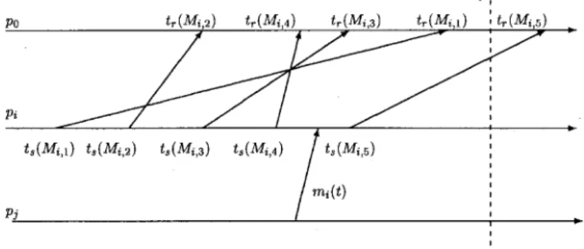
This appendix proves Theorem 5; that is, we show the correctness of our DT detection algorithm. In this appendix, the term “messages” means data messages or the messages sent in the Time Warp simulation, and the term “reports” means idle messages sent for DT detection. Let ts(m) be the (real) time when a message/report m is sent. Let tr(m) be the (real) time when a message/report m is received. We assume that tr(m) > ts(m) (i.e., non-zero message sending delay). Let Mi,k be the kth report sent from pi.
Definition 11: Mi(t) = Mi,k is called the last effective report of process pi at time t if and only if tr(Mi,k) < t and for all k', tr(Mi,k') Π[tr(Mi,k), t], we have k' < k.
Fig. 7. The timing diagram for Lemma 5. Fig. 6. An example of the last effective report.
Definition 12: The first message which re-activates process pi after pi sends Mi(t) is denoted as mi(t).
In Fig. 6, Mi(t) = Mi,4 is the last effective report of pi at time t, and mi(t) re-activates pi after Mi(t) is sent.
Lemma 5: Suppose that p0 satisfies the DT condition at time tT, and for all piΠP, let Mi(tT) be the last effective report of pi at time tT. Then pi is idle in the time interval [ts(Mi(tT)), tT].
Proof: We prove by contradiction. Suppose that pi is active in (ts(Mi(tT)), tT]. Then pi receives (and is re-activated by) a message mi(tT) after time ts(Mi(tT)). Suppose that mi(tT) is sent by pj. Let mi(tT) be the lth message sent from pj to pi. Since r'i,j(tT) = ri,j(ts(Mi(tT))) < l and s'j,i(tT) = r'i,j(tT), we have l > s'j,i(tT). This implies that ts(mi(tT)) > ts(Mj(tT)), that pj must be re-activated by a message mj(tT) in the interval (ts(Mj(tT)), ts(mi(tT))), and that
Fig. 8. The timing diagram for Lemma 6.
(cf. Fig. 7) Thus, for every active process pil, there always exists another active process pil+1 such that tr(mil+1 (tT)) < tr(mil(tT)). In other words, we can find an infinitive sequence i1, i2, ...,
il, ... such that
tr(mi1(tT)) > tr(mi2(tT)) > ... > tr(mil(tT)) > ...
Since |P| is finite, we have pil = pin for some n < l. Without loss of generality, let n = 1. Then we have
tr(mil(tT)) > tr(mi2(tT)) > ... > tr(mil-1(tT)) > tr(mil(tT)) = tr(mil(tT)),
a contradiction. o
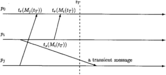
Lemma 6: If p0 satisfies the DT condition at tT, then there is no data message in transit.
Proof: We prove by contradiction. Suppose that a message sent from pi to pj is in transit at time tT. pi(pj) is idle in the intervals [ts(Mi(tT)), tT]([ts(Mj(tT)), tT]), where Mi(tT)(Mj(tT)) is the last effective report at tT (From Lemma 5). Thus, si,j(tT) = s'i,j(tT) and rj,i(tT) = r'j,i(tT). Since the transient message must be sent before ts(Mi(tT)) (Lemma 5, and pj has not received the message at time tT), we have rj,i(tT) < si,j(tT) (cf. Fig. 8). This implies that r'j,i(tT) < s'i,j(tT), which contradicts the DT condition.
Thus, Theorem 5, (i.e., the system terminates when p0 satisfies the DT condition) is a
direct consequence of Lemmas 5 and 6. It is apparent that this algorithm is optimal in time complexity:
Theorem 8: Suppose that a process pi is idle forever after time tpi. Let Dtpi be the message sending delay of the report pi sends at time tpi. Then p0 reports distributed termination at
time max( )
∀i tpi+∆tpi .
From Theorem 5, our algorithm satisfies the safety property (that is, no false termina-tion is detected). From Theorem 8, our algorithm satisfies the liveness property (that is, after the system terminates, the termination is detected in finite time).