Subscriber access provided by NATIONAL TAIWAN UNIV
Industrial & Engineering Chemistry Research is published by the American Chemical Society. 1155 Sixteenth Street N.W., Washington, DC 20036
Evaluation of the process transfer function using partial pulse response data
Chih Chuan Huang, and Cheng Ching YuInd. Eng. Chem. Res., 1989, 28 (9), 1304-1308 • DOI: 10.1021/ie00093a007 Downloaded from http://pubs.acs.org on November 28, 2008
More About This Article
The permalink http://dx.doi.org/10.1021/ie00093a007 provides access to: • Links to articles and content related to this article
1304 I n d . Eng. C h e m . Res. 1989,28, 1304-1308
PROCESS ENGINEERING AND DESIGN
Evaluation of the Process Transfer Function Using Partial Pulse
Response Data
Chih-Chuan Huang and Cheng-Ching Yu*
Department of Chemical Engineering, National Taiwan Institute of Technology, Taipei, Taiwan 10772, R.O.C.
A
method is proposed t o identify th e dynamic models of plants from only a pa rt of t he process response. This method requires only a visual inspection of Bode plots constructed from the Fourier transform of partial (truncated) pulse response data. An extremely accurate approximation of time constants can be obtained for a truncation time/time constant ratio as small as 1/4. A complete procedure for evaluating transfer functions is also presented.In the application of advanced control strategies, the mathematical description of the plant dynamics, e.g., its transfer function, must be known as exactly as possible. Process identification can achieve the purpose by finding the process model from experimental plant tests. A num- ber of techniques in process identification have been proposed. Pulse testing (Luyben, 1973) is often used to identify chemical processes because of its simplicity and minimal upset to the operating plant. A pulse change is made in the manipulated variable, and the pulse response of the controlled variable is recorded. Bode plots are constructed from the Fourier transformed pulse response data. The process transfer function can be evaluated from the Bode plot. This topic is discussed in detail by Luyben (1973). In theory, we need the complete pulse response data, i.e., the controlled variable comes back to its starting value, to perform Fourier transformation in order to get the correct Bode plot of the process model. However, in an operating environment, it is nearly impossible to get complete pulse response data for the following reasons: (1) the controlled variable deviates from the set point for a long period of time and (2) it is extremely difficult to maintain the same operating conditions over such a long period of time. This is especially true for processes with long time constants, e.g., high-purity distillation column (Fuentes and Luyben, 1983).
Moudgalya et al. (1987) proposed a dual-pulse method to overcome this problem. A second pulse with the sign opposite to the first pulse is introduced at a different time to reduce offset in the controlled variable. Despite the success in reducing the offset, the time required to com- plete the dual-pulse testing remains significant. The purpose of this work is to identify the process transfer function using only partial, namely, truncated, pulse re- sponse data.
This paper is organized as followings. The Laplace and frequency responses of the truncated impulse response data are derived followed by extracting dynamic infor- mation from frequency responses of the truncated pulse response data. A procedure for deriving the process transfer function is also presented.
Tra n s fo r m at io n of T r u n c a t e d P u l s e Response D a t a
In theory, we need the complete pulse response data (Figure 1) to reconstruct frequency responses, i.e., Eode
plot, in order to derive the process transfer function. However, in any practical situation, it is nearly impossible to have the entire pulse response data without facing disturbances from load variables or other manipulated variables. Therefore, in most cases, the pulse response data are truncated one way or the other.
Consider the following process
G(s) = X ( s ) / M ( s )
where X ( s ) is the output variable and M ( s ) is the input variable. If an impulse input is applied to the input variable, i.e., m(t) = 6 ( t ) (a delta function), the impulse response can be Laplace transformed to obtain the original process model G(s). By definition, we require the impulse response to go to infinity in order to extract the exact dynamic information:
X ( s ) = L m r ( t ) e + dt (1) and
G(s) = X(s)/l (2)
As mentioned earlier, in practice, only T minutes of im- pulse response are taken (Figure 1). The process model becomes
(3) For a simple first-order lag process,
The impulse response truncated a t time T gives
where 7 = e-T/*. The relationship between G(s) and
b(s)
is
d ( s )
= (1 - ve-Ts)G(s) (6) Clearly, a mismatch between the approximated model(b)
and the true process ( G ) exists. The discrepancy is the 0888-5885/89/2628-1304$01.50/0 0 1989 American Chemical SocietyInd. Eng. Chem. Res., Vol. 28, No. 9, 1989 1305
0 100 2M) E00
nm. ( mi". )
Figure 1. Pulse response of a first-order system.
result of incomplete (truncated) impulse response data. Taking the same-approach, we can get the relationship between G(s) and G(s) when the change is a pulse input. The height and duration time of the pulse input is unity and D, respectively; i.e.,
m ( t ) = u ( t )
-
u(t -D )
(7) (8) 1M ( s ) = -(1
-
e-D8)where u ( t ) is the unit step function. The pulse response becomes
S
KP 1
X ( S ) = G ( s ) M ( s ) =
-
-(1 - e-DS)r s + l s
When only T-min response data are taken,
T
8 ( s )
=1
Kp(l - e - t / T ) e - 8 t dt - G(s) = z ( s ) / M ( s ) = G ( s ) ( l-
Te-Ts) (11) where T e - T l r ( e D / r - 1) 7 = (12) -(1 -Again, a similar type of mismatch exists between G(s) and (3s).
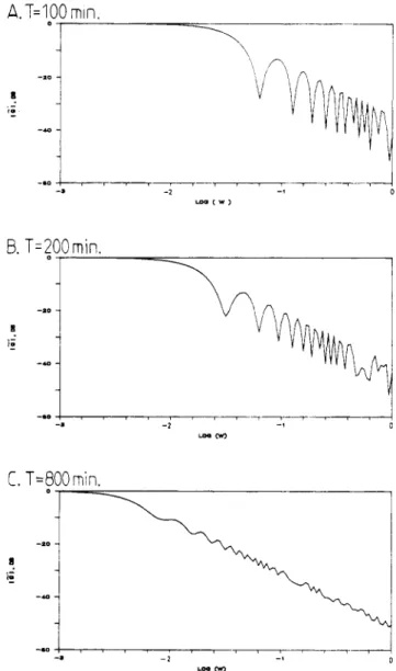
In the preceding paragraph, the analytical expression for the transfer function is derived from the truncated pulse (or impulse) response data. In a plant test, however, the pulse response data are Fourier transformed, and a Bode plot is constructed from the Fourier-transformed response data (Luyben, 1973). Figure 2 shows such a Bode plot from pulse testing results for the response data truncated at T = 100,200, and 800 min, respectively. The process is a first-order lag with time constant of 400 min, which is a relatively slow process. Unlike the conventional Bode plot, the experimentally obtained Bode plots (Figure 2) from truncated pulse response data show significant wiggling especially in the high-frequency range. The ali- asing effect is more profound as we shorten the truncation time (Figure 2A). The oscillatory behavior in the Bode plot was often found in identifying the high-purity dis-
S
A.T=100
min.
O 1 - \ - -I
i
9 .- ' 0C.
T-800min.
O 1 - - - ---1o-
9 .- 'D -a-
-
- 1 -.o-.
- 2 =emFigure 2. Bode plots of C(s) = 1/(400s
+
1) for pulse response truncated at (A) T = 100 min, (B) T = 200 min, and (C) T = 800 min.tillation process (via pulse testing of a rigorous nonlinear dynamic model). I t was often thought to be the result of strong nonlinearity in the process. It is clear that the oscillatory behavior is the result of truncated pulse re- sponse data.
Extract Dynamic Information
An important question remains. Can we extract rea- sonable dynamic information from these Bode plots (Figure 2)? A popular approach is to use the least-squares method (Stahl, 1984) where coefficients (e.g., time con- stants) of a transfer function are found by fitting frequency response data to a given structure. However, the least- squares method fails for short truncation times (e.g., T = 100 and 200 min) as shown in Figure 3. For T = 100 min (Figure 3A), the least-squares method underestimates the time constant by a factor of 5 (Table I).
A simple method is proposed that enables the designer to visualize the time constant (high-frequency asymptote) rapidly. All the designer ought to do is to draw an high- frequency asymptote to the successive minima in the Bode plot as shown in Figure 3. The corner frequency (the intersection of low- and high-frequency asymptotes) in the Bode plot is the reciprocal of the time constant. Extremely accurate estimation of the time constant is obtained for truncation times of 100, 200, and 800 min (Table 1). The
1306 Ind. Eng. Chem. Res., Vol. 28, No. 9, 1989
A
T=103
min A. em 0 7 I -0 1 - , T = Z i U m- - -
in - . o t - 7 7 - - - ,-.
, , ,---a
- 2 - 1 C LOO ( w,
Figure 3. Comparison of least-squares and proposed methods in extracting dynamic information for truncation time T (A) T = 100 min, (B) 7' = 200 min, and (C) T = 800 min. (1) Results from the least-squares method, (2) true model, and (3) results from the pro- posed method.
reason for such an accurate estimate is explained as follows. The mismatch (e,) between the true proces? dynamic (G')
and the approximated dynamic model (G') can be ex- pressed as
where the superscript ' denotes the normalized transfy function, i.e., G'(0) = 1. For the first-order lag system, G ' becomes
For the first-order lag example with truncation time T , e,
can be written as
The magnitude plot of e,(iw) (Figur- 4A) shows that the smallest multiplicative error ((G'- G')/G') occurs a t the
8 f , - 4 - / -8
p
'
- ' 21
-1L 4 -20i
1 -24 * ?I----Figure 4. Multiplicative modeling error, e,, for a truncation time of 100 min (A) and the corresponding Bode plots for G and G' (B). lowest part of the oscillation. Therefore, the successive minima in the Bode plot possess the most accurate in- formation about the true process as shown in Figure 4B. Thus far, we have dealt with idealized responses (Figure 1). In practice, the pulse response data are often corrupted with process and/or measurement noises. In order to test the reliability of the proposed method in an industrial environment, the pulse response data are corrupted with different levels of random noise (Figure 5). For a trun- cation time of 100 min, the process time constant still can be accurately identified through the successive minima in the Bode plots (Figure 6).
The proposed method can identify the time constant and order of the system with only a part of (truncated) the pulse response in an industrial environment. A general transfer function consists of three parts: (1) time constant, (2) dead time, and (3) steady-state gain. Dead time can be observed from the initial part of the time-domain re- sponse. For conventional pulse testing, the steady-state gain is the area under the response curve. For the pro- posed method, however, the steady-state gain can be back-calculated by fitting the response curve with a known time constant and dead time (Moudgalya et al., 1987).
The procedure for evaluating transfer functions can be summarized as follows: (1) introduce the pulse input and truncate the response data in an endurable limit by the plant, (2) evaluate the truncated pulse response data by Fourier transform and construct the Bode plot (Luyben, 1973), (3) evaluate the time constants with the proposed method, (4) observe the dead time from the time-domain response data, and (5) back-calculate the steady-state gain by fitting the time-domain response to the known dynamic
Ind. Eng. Chem. Res., Vol. 28, No. 9, 1989 1307
A
Table I. Comparison of Different Methods To Evaluate the Process Time Constant with Different Truncation Times
(T)
7 , min'
T , min least squares proposed method
100 78.8 360
200 144.7 370
800 358.5 400
'The true process time constant is 400 min.
i
B.
C.
0.000. I 0 100 2w 800 nm. ( nm.,Figure 5. Pulse responses of a first-order system corrupted with
white noises of different covariances.
information, i.e., time constants and dead time. Conclusions
A simple method is proposed to evaluate the process time constants from the truncated pulse response data. This method involves only visual inspection of the Bode plot and does not require any calculation. Extremely ac- curate results were obtained with relatively short trunca- tion times, e.g., the truncation time is only one-fourth of the process time constant. Th e proposed method works reliably even when the pulse response data are corrupted with process and/or measurement noises. This method is especially useful for processes with long time constants, and deviations from set point cannot be tolerated for a long period of time. 9 .- " -, - . o !
-.
, , , , , , , , , -2 0 L o O ( W ) n -, -sa-.
-2 W ( - )Figure 6. Bode plots for pulse responses corrupted with different levels of white noise for a truncation time of 100 min.
Acknowledgment
This work is supported in part by National Science Council of the R.O.C. under Contract NSC-76-0402-E- 011-04.
Nomenclature
D = duration time of pulse input
e , = multiplicative modeling error, (C'-
G r ) / G r
G = process transfer function
C '
= normalized process transfer function G = approximated process transfer functionG
'
= normalized approximated process transfer function, Le.,@I
= magnitude ofG
K , = steady-state gainm = manipulated variable
M = Laplace-transformed manipulated variable
s = Laplace transform variable
T = time period where pulse response is truncated (truncation u = unit step function
x = controlled variable
X = Laplace-transformed controlled variable
Greek Symbols
T = time constant, min
Gf(0) = 1
1308
w = frequency, r a d / m i n
Ind. E n g . Chem. Res. 1989, 28, 1308-1324
Moudgalya, K. M.; Luyben, W. L.; Georgakis, C. A Dual-Pulse Me-
Literature Cited
thod for Modeling Processes with Large Time Constants. Ind. Eng. Chem. Res. 1987,26, 2498.
Stahl, H. Transfer Function Synthesis Using Frequency Response - . . Data. Int. J . Control 1984,-39, 541.
Fuentes, C.; Luyben, W. L. Control of High-Purity Distillation Column. Ind. Eng. Chem. Process Des. Deu. 1983, 22, 361.
Luyben, W. L. Process Modeling, Simulation and Control for Chemical Engineers; McGraw-Hill: New York, 1973.
Received f o r review October 14, 1988 Revised manuscript received April 24, 1989 Accepted J u n e 8, 1989
Continuous Solution Polymerization Reactor Control. 1. Nonlinear
Reference Control of Methyl Methacrylate Polymerization
Derinola K. Adebekun and F. Joseph Schork*
School of Chemical Engineering, Georgia I n s t i t u t e of Technology, Atlanta, Georgia 30332-0100
This paper focuses on nonlinear control of a solution polymerization reactor via a reference controller. A stability and convergence analysis shows that global stabilization of the reactor is possible under certain conditions. It is also demonstrated th at, for certain equilibrium points, input multiplicity exists in the controlled subset of the system state, and this is detected by the controller in the closed loop.
Introduction
Polymerization reactors are known to exhibit strong nonlinearities (Knorr and O’Driscoll, 1970; Hamer e t al., 1981; Schmidt e t al., 1984; Schmidt and Ray, 1981) and pose difficult control problems. In particular, the molec- ular weight distribution (MWD) also has to be maintained in order to produce polymers of acceptable quality. Typically, the MWD is characterized by the first few leading moments of the distribution. From these moments, typical measures of polymer quality, which include the number-average chain length ( F ) and the polydispersity
(D),
can be computed. Methods for doing this are dis- cussed by Ray (1972). Furthermore, in continuous plants, the desired distribution may occur only at equilibrium points where the reactor is open-loop unstable. Indeed, as is demonstrated in Adebekun et al. (19881, it is possible that all equilibrium points corresponding to a given MWD are open-loop unstable. Thus, the control systems for these reactors should be able to give offset-free performance over a wide range of operating conditions.As can be expected, the control of polymerization re- actors has attracted some interest in the literature. Most of the earlier works involved some form of optimal control, in particular, for batch and semibatch polymerizations. Typical case studies include the papers by Hicks et al. (19691, Osakada and Fan (1970), and Hoffman et al. (1964). In CSTR polymerization, much can still be achieved from a control standpoint. Most of the work in this area involves designs based on the traditional Taylor series linearization (or its variant) about some base point. Even so, good results are possible with this approach. Examples of these can be found in the work of Tanner et al. (1987) and Congalidis et al. (1986).
More recently, advances in nonlinear systems theory have led to the development of nonlinear control synthesis techniques. Some of these results have been applied to polymerization reactor control. Thus, Alvarez et al. (1988) and Kravaris and Soroush (1988) have applied differential geometric methods to both continuous and batch polym- erizations, respectively. Some other nonlinear applications
* T o whom all correspondence should be directed.
0888-5885/89/2628-1308$01.50/0
involve the work by Marini and Georgakis (1984). How- ever, more experience is required in this area for rational control system design. Other approaches involve adaptive control techniques. This is typified by the work of Kwalik and Schork (1985).
In this work, we approach the control problem via a reference controller approach. These ideas for nonlinear process control are becoming increasingly important and appear to have been proposed by Boye and Brogan (1986). Subsequent work on this has been presented by Bartusiak et al. (1988). Under certain conditions, we are able to guarantee global asymptotic stability. Furthermore, we establish contact again with bifurcation theory in the guise of the c a t a s t r o p h e set and demonstrate the importance of reactor “psychoanalysis” in design applications (Bilous and Amundson, 1955). The relationship to bifurcation theory is in fact not new. It was first pointed out in a control framework by Koppel (1982). Koppel’s observa- tions have since been further generalized by Balakotaiah and Luss (1985). In particular, for polymerization reactors, the important implications of input multiplicity are first brought to light. It is interesting to note that even without integral action, the controller is able to detect the existence of input multiplicity. Indeed, this is consistent with the results of Balakotaiah and Luss (1985) in that input multiplicity is a property of the system and n o t of the controller.
In part 2 of this work (Adebekun and Schork, 1989), in order to motivate realistic evaluations, we incorporate a Kalman filter in latter design stages for reconstruction of unavailable state variables. The robustness of the scheme to filter errors is then evaluated via simulations. Model
The polymerization of methyl methacrylate proceeds by a free-radical mechanism. The solvent is ethyl acetate, while the initiator is benzoyl peroxide. The reaction is highly exothermic and has been the object of some study (Schmidt and Ray, 1981). In the interest of brevity, we merely state that the following model equations hold (Schmidt and Ray, 1981; Tanner et al., 1987):
VM = q ( M f - M ) - Vk,MP (1) IC 1989 American Chemical Society