運動模擬器之運動控制的ECAM追蹤法則

行政院國家科學委員會補助專題研究計畫成果報告

※※※※※※※※※※※※※※※※※※※※※※※※※

※ ※

※ 運動模擬器之運動控制的 ECAM 追蹤法則

※

※ ※

※ ※

※※※※※※※※※※※※※※※※※※※※※※※※※

計畫類別：

個別型計畫

整合型計畫

計畫編號：NSC 91-2212-E-009-050-

執行期間：91 年 08 月 01 日至 92 年 07 月 31 日

計畫主持人：成維華 教授

本成果報告包括以下應繳交之附件：

□赴國外出差或研習心得報告一份

□赴大陸地區出差或研習心得報告一份

□出席國際學術會議心得報告及發表之論文各一份

□國際合作研究計畫國外研究報告書一份

執行單位：交通大學機械工程研究所

中 華 民 國 92 年 8 月 31 日

行政院國家科學委員會專題研究計畫成果報告

計畫編號：NSC 91-2212-E-009-050-

執行期限：91 年 8 月 1 日至 92 年 7 月 31 日

主 持 人：成維華 交通大學機械工程研究所

Multi-axis coordinated trajectory following is important in CNC machines and metal cutting tools. Recently, flight simulators with electrical actuators have been in increasing demand. However, the coordinate control scheme affects the accuracy of the motion because motors have an insufficient load capacity relative to the hydraulic actuators. The electronic cam (ECAM) is typically used to perform coordinated control. However, selection of the master may determine potentially very different characteristics of motion. This study proposes an automatic master switching method. The conditions and results of the master switching method for electronic cam are detailed. The robustness and stability of the proposed control system is also

demonstrated using the well-known structured perturbation analysis tool,  .

Keywords: multi-axis coordinated trajectory

following; electronic cam; robustness; stability; structured perturbation analysis

二、緣由與目的

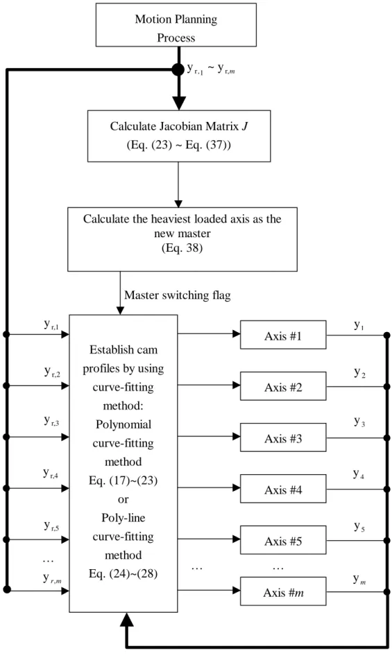
Electronic cam (ECAM) tracking is applied to a multi-axes motion control system mainly to enable the slaves to follow consistently trajectories obtained from the predicted sets of reciprocal points of master and slaves. When the master receives a position command, it will or will not be driven to the desired position, and the slaves will be moved into new positions by following the predicted cam profiles. However, in a fixed master ECAM system, the heavily loaded slaves may follow a lightly loaded master, and then the slaves may lose tracking precision as it reaches its current (force) limit. Kim and Tsao (2000) developed an electrohydraulic servo actuator for use in electronic cam motion generation, addressing the robust performance control for the fixed slave, an electrohydraulic servo actuator. Steven (1995) specified a tracking control electronic gearing system called an “optimal feed-forward tracking controller”, primarily associated with the fixed slave controller design. Each of their control schemes was demonstrated to satisfy the demands of precision and robustness, but to be valid only for its particular application. This study introduces a master switching control scheme, as shown in Fig. 1, to specify the generalized ECAM control problem.

In the master switching control scheme, the most heavily loaded axis must be predetermined before anticipative motion begins: this axis will be treated as the master

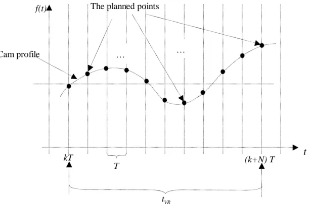
and the other axes as the slaves. The master may be switched between different types of motion from time to time, to exchange the master and one of the slaves in the subsequent action. After the master is instantaneously determined, the next important task is to build ECAM profiles from the demanded ECAM tables. Two curve-fitting methods (Dierchx & Paul, 1993) are proposed to establish piecewise ECAM profile. One is the polynomial curve-fitting method, as shown in Fig. 2, which is suggested for use in cases of low frequency motion. Simulations indicate that the polynomial curve-fitting method (Chen, 1995) (Reich, 1992) performs well, if the frequencies of the active body are less than one-tenth of half of the system’s sampling frequency (Nyquist frequency). Restated, this method is favorable if and only if the trajectory of motion is very smooth from the viewpoint of the Nyquist frequency. The second method is the poly-line curve-fitting method, as shown in Fig. 3, which is more appropriate for higher frequency motion.

A six degree-of-freedom (DOF) motion simulator SP-120, shown in Fig. 4, was used to implement and prove the robustness and stability of the proposed master switching control system. The important issue of the robust stability of a six DOF motion simulator concerns its six-axes cross-coupled behavior: each axis pulls and drags every other such that the most heavily loaded axis may act unexpectedly; that is, the actual trajectory of the cockpit may be unexpected. This phenomenon follows from inconsistent tracking of the planned trajectory and may cause the cockpit of the motion simulator to leave its nominal workspace. Thus, a robust positioning controller is urgently required. Several articles have referred to the design of controllers of six DOF motion simulators. Chung, Chang and Lin (1999) referred a fuzzy control system for a six DOF simulator and considered the hydraulic actuator system. Werner (1996) introduced a robust tracking control for an unstable, linearized plant which was linearized. Plummer (1994) described a nonlinear multi-variable controller for a motion simulator. The procedure for completely designing a robust controller of a nonlinear system consists of

finding the nominal controlled plant (Kim & Tsao, 2000) (Dixon & Pike, 2002) (Zhiwen & Leung, 2002) (Al-Muthairi, Bingulac & Zribi, 2002), which is very complicated and impractical; thus, the dynamics of the nonlinear control system must be linearized and simplified. Simplified dynamics of the simulator SP-120 are proposed to model the structured perturbation with parametric uncertainties. The well-known  tool (Zhou, 1998) is used to analyze the robust performance of the original control system, and then to demonstrate that it is more robust and stable after the proposed control scheme is applied to the system.

Real-time software was developed to implement the PC-based master switching ECAM control scheme used in the SP-120 motion simulator (Fig. 4). Experimental results show the advantage of the proposed tracking accuracy. However, experimental analysis has also revealed that a shorter system sampling time yields more accurate tracking control, especially when the poly-line curve-fitting method is used. However, a tradeoff exists between the system sampling time and the calculation burden in a programming cycle.

三、研究報告內容

1. Method of Building Cam Profiles (Master-slaves Trajectories)

1.1 Polynomial curve-fitting

A polynomial curve-fitting method is proposed to build a continuous curve in order to fit a known discrete signal, and the established curve is treated as the piecewise-continuous cam profile (master-slaves trajectories). As presented in Fig. 2, T is the sampling time of the driving system and t_VR is the period of motion planning. The predictive planned N points are the known discrete commands for which t _VR equals N times T; the cam profile of each axis can be expressed as a function of time index t, which describes the common relationship between master and slaves, for 0t NT, and      1 0 , ) ( N n n n i i t c t f , i = 0 to m (1) in which m is the numbers of axes. By expanding Eq. (1), then

i i matrix i i i N i i i N N F C T T N f T f f c c c T N T N T T                                                ) ) 1 (( ... ) ( ) 0 ( ... ] ) 1 [( ... ) 1 ( 1 ... ... ... ... ... 1 0 ... 0 1 1 , 1 , 0 , 1 1 i matrix i T F C    1 (2) where f_i(t) is the position of the

i

matrix

T , C and _i F are the constant time _i matrix, the polynomial parameters of the th

i axis and the predicted positions of the

i

Adequately estimating the master’s next position f_m(t) enables the above equation to be used to determine the time index t, and then the estimated positions of all of the slaves are determined by substituting t into Eq. (1). The algorithm includes the following steps.

1. Estimating the next position of the master is an electronic gearing process, and the proper estimate is expressed follows.

T v x x t f_m(ˆ_k1) ˆ_k1  _k  ˆ_k (3) where xˆ_k1 is the estimated position of the master; x_k  y_k is the present measured position of the master, and vˆ is the _k velocity estimated during the process of motion planning.

2. Substituting the estimated position xˆ_k1 of the master into Eq. (1) yields,

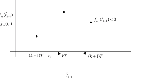
         1 0 1 1 1) ˆ ˆ ˆ ( N n n k m k k m t x c t f (4) This equation generally has N-1 solutions, and only one real rational solution is correct. A proper constraint tˆ_k tˆ_k1 (k1)T is added to Eq. (4) to limit the region in which the solution may be found. Sometimes, two solutions satisfy this constraint, but identifying the correct one is not difficult.

According to the properties of the polynomial curve and the planned velocities of the master, the sign of the slope of the curve plotted against the time index

t

ˆ

k

vˆ . For example, in Fig. 6, the solution near (k+1)T is the correct one.

The master velocity in terms of the time index

t

ˆ

          1 0 1 1 1 1 ' ˆ d / ˆ d ) ˆ ( N n n k m k k m t x t nc t f (5) such that, ) ˆ ( ) ˆ ( 1 0 1 1 k N n n k m t sign v nc sign       (6) where,              zero is as negative is as positive is as sign ) ( , 0 ) ( , 1 ) ( , 1 ) (

3. The time index is estimated in the preceding steps, and the estimated position of the i slave is represented as, th

n k N n in k s i t C t f 1 ₁ 0 , 1 , (ˆ ) ˆ      , i = 1 to 5 (7) 1.2 Poly-line Curve-Fitting

The poly-line curve-fitting method is used to fit the signal of higher frequency according to the viewpoint of Nyquist frequency. And then yields a poly-line curve as shown in Fig. 3. If the number of motion planning points equals N, then as in the section 2.1, the cam profile can be expressed as a function of the time index t.

      1 0 , ) ( N n in i t c t nT f , i = 0 to m (8) Expanding Eq. (24) yields

i i matrix i i i N i i i F C T T N f T f f c c c T N T N T N T T N T                                                ) ) 1 (( ... ) ( ) 0 ( ... 0 ... ) 2 ( ) 1 ( ... ... ... ... ) 2 ( ... 0 ) 1 ( ... 0 1 , 1 , 0 ,

i matrix i T F C    1 (9) where the parameters in Eqs. (8) and (9) are all defined as in the above section. Similarly, matrix T_matrix is constant and nonsingular; thus, T_matrix1 exists.

The next time index

t

ˆ

Case 1: 0t_k1T 1 1 1 1 1 1 0 ) ˆ (  _          k N i i k N i i x T ic t c c Case 2: T t_k1 2T 1 1 2 1 1 1 2 1 0 ˆ ) ( ) (  _              k N i i k N i i i i x T ic c t c c … Case N-1: (N 2)T t_k1 (N1)T 1 1 2 1 1 1 2 0 ˆ ) ) 1 ( ( ) (                 k N N i i k N N i i x T c N ic t c c

Under these conditions, the general formulation is as follows. ] ) ˆ ( [ ] ) ˆ ( ˆ [ ˆ 1 0 1 1 1 1 1 1                 N n n k N n k n k k nT t sign c nT c nT t sign x t (10)

This equation is solved first by determining whether the value of (tˆk1nT)

is positive or negative. Restated, the probable region of tˆk1 must be determined correctly. The region t_k tˆ_k1 (k1)T is the correct choice, where t is the actual time index _k obtained by substituting the actual master’s position x into Eq. (10) at time kT. Multi _k solutions may be in this region, so the correct solution of Eq. (10) must next be identified. As aforementioned, the sign of the slope of the poly-line function of the time index tˆ_k1

must be the same as that of the ideal velocity

k vˆ . That is, ) ˆ ( ) d / ) ˆ ( d ( f tk 1 t sign vk sign _  (11) From the above analysis, the time index

1

ˆ_

k

t can be estimated; then, the estimated position of the i slave can be represented th as,         1 0 , 1 1 , (ˆ ) ˆ N n ni k k s i t c t nT f , i = 1 to 5 (12)

2. Infinity Norm of the Master Switching ECAM Controller

The control input of the master switching method can be expressed as yr tTmatrixr

1 , where r is the reference displacement input. Then, from the characteristics of the master switching ECAM control scheme, the actual speed of each axis theoretically does not exceed its reference speed. Therefore, the reference displacement y is confined by _r

| | |

|yr  r ; that is, the infinity norm of the controller (tTmatrix1 ) is confined by,

1 ||

||_tT_matrix1 _ (13)

3. Applying the Proposed Control Scheme to a Six DOF Motion Simulator

This proposed master switching ECAM control scheme is applied to the control system of multi-axes mechanisms to demonstrate its advantages. In this paper, the six DOF motion simulator SP-120 (Fig. 4) is used to implement the generalized ECAM tracking technique. If the current (force) of the most heavily loaded axis reaches its critical value, then the cockpit cannot easily execute its planned motion easily by directly feeding individual, planned commands to each axis. Rather, the cockpit may sometimes leave its nominal workspace. Accordingly, the master switching ECAM control scheme is better suited than the master fixed ECAM method to this application.

The master of the motion simulator is predetermined the heaviest loaded axis, so the Jacobian matrix (John, 1989) of the simulator must be calculated and updated from time to time. Appendix A presents the detailed algorithm for finding the master.

4. Analysis of Stability and Robustness

The dynamics of each slider of the SP-120 motion simulator (Figs. 4 and 5) can be modeled by parametric uncertainties, using the linear fractional transformation (LFT) representation. An equivalent mass, m, is introduced to simplify the dynamics of the slider motion and to decouple the components of the system’s nonlinear terms, to explicate the stability and the robust

performance of the system. Thus, a simplified dynamic model of each slider is,

c c n p K K E s u       _{2 /}  _{, (14)} where x sp/2 is the displacement of

each slider; c c f nx K K E K u  (15) where Kf sp/2 is the machine constant.

As presented in Fig. 7, m u x m c x( / ) /  (16) in which the parameters in Eqs. (14) ~ (16) are defined in the nomenclature. Suppose that the physical parameters m and c are not known exactly, but are believed to lie in known intervals. Assume,

c c m m c c m m   ,    (17) where the nominal mass is

2 / ) (mH mL

m   , and the nominal damping is c (c_H c_L)/2; the maximum variation of mass is m (mH mL)/2, and the maximum variation of damping is

2 / ) ( _{H L} c  c c  ; the perturbations  _m and  are confined by _c |_m|1 and

1 | |_c  , respectively, in which m =250 kg, _H s kg c_H 15 / and m = 50 kg, _L c_L 5kg/s are in practice the upper and lower bounds of the slider’s nominal mass and damping, respectively.

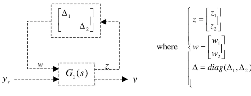
Figure 8 presents the system’s block diagram according to the foregoing dynamical equations. Suppose the control input is T

2 1, , ]

[w w y_r and the output is T

2 1, , ]

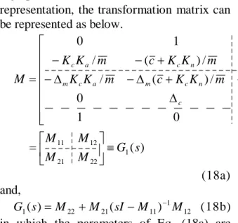
[z z y . Then, using the Doyle’s representation, the transformation matrix can be represented as below. ) ( 0 0 0 0 1 0 0 0 0 / / / / ) ( / / / 1 / 1 / ) ( / 0 0 0 1 0 1 22 21 12 11 s G M M M M m K K m m m K K c m K K m K K m m m K K c m K K M c a c m m m n c m a c m a c n c a c                                          (18a) and, 12 1 11 21 22 1(s) M M (sI M ) M G     (18b) in which the parameters of Eq. (18a) are

defined in the nomenclature, and the system

including the perturbations  and _m  , can _c be represented using LFT. That is,

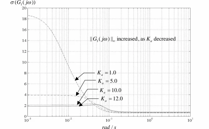
             M y RH y c m r u   , ) , ( , z z z w w w _                 2 1 2 1 (19) where  M_u( ,) is the upper LFT, as shown in Fig. 9, and  RH is the  _ structured uncertainty. Stability is often not the only property of a closed-loop system that must be robust to perturbations. The most well-known use of  as a robustness analysis tool is in the frequency domain. Figures 10 and 11 show the singular value frequency responses of G₁(j) and the structured singular values, _(G₁(j)) , respectively, for each frequency with

2 2 

 C , obtained by adjusting the proportional gain, K . These figures are _a obtained by programming the theorem of  (Zhao, 2000). Moreover, the bounds of

)) ( ( ₁ 

_ G j are formulated within the reference book (Zhou, 1998). In Figs. 10 and 11, the maximum singular value of G₁(j) is increased by decreasing the proportional gain, and the maximum structured singular value is increased by increasing the proportional gain. Table 1 presents the maximum singular values G₁(j)_ , the maximum structured singular values

)) ( ( sup ₁   R G j 

 and the bandwidth of the control system for various proportional gains. Moreover, if the upper bound of the nominal mass exceeds a critical value, then the maximum structured singular value will be larger than unity, possibly causing the requirement for robust performance to be unsatisfied. Table 2 presents the critical upper bounds of m_H for various proportional gains, K . The critical upper _a bound increases as the proportional gain decreases. Combining Table 1 and Table 2 reveals that the system is more robustly stable at a lower proportional gain, but the time constant of the system responses is higher. Thus, a tradeoff exists between the robustness and the performance of the system’s response. Nevertheless, by carefully

considering this tradeoff, the most suitable proportional gain can be conveniently adjusted to fit the specific demands of the control. In this paper, m is estimated to be H

around 250 kg by transforming the maximum torque of each joint of the motion simulator SP-120 to the equivalent mass. The maximum torque is obtained by applying the critical velocity and the maximum tolerable acceleration to drive the slider of the motion simulator provided traveling most the nominal workspace of the simulator. Moreover, for example, if the damping ratio is set to 0.707, then the proportional gain must be adjusted to 6.3, and the maximum structured singular value is then calculated as 0.801358. Clearly, the sufficient and necessary condition for robust performance is satisfied. That is, the maximum structured singular value must be less than unity. Consequently, according to the theorem of  and  -synthesis, the system is well-defined and internally stable under the structured perturbation,  _ 1.

By combining Eq. (13) with the above results, the maximum structured singular value of the entire system, G₁G₂, is confined by the following inequality.

1 )) ( ( sup )) ( ) ( ( sup 1 2 1   _           j G j G j G R R (20)

Restated, the master switching control system is more robustly stable than the original stable system.

5. Numerical Method for the Forward Kinematics of Six DOF Motion Simulator

The cockpit trajectories obtained using conventional tracking control and the proposed tracking control, are compared to demonstrate the precision of the proposed control scheme. Therefore, the six sliders must be transformed into the cockpit positions off-line; that is, forward kinematics will be used to transform the six axis coordinates into the cockpit’s coordinates, including translation components and rotation components (and representing a transformation from J to S). However, direct forward kinematics is difficult to formulate for a six DOF motion simulator. Therefore, this study proposes the use of a numerical

method, such as Newton’s method to execute the transformation (J to S) indirectly. The following iterative steps describe the numerical, steepest descent approach (Garret, 1984) (Edwin & Stanislaw, 1996).

1. Set k 0 , and set the initial cockpit position, x , to the cockpit home position. ₀ 2. Calculate the present Jacobian matrix J , _k according to the algorithm presented in the Appendix A.

3. Calculate the estimated errors in the positions of the six sliders as,

6 , R p p_{y estk} k     (21) where py is the actual position of one

slider, p_est,_k is the estimated positions of the six sliders, calculated by inverse kinematics, and  is the chosen step _k size.

4. Calculate the next estimated cockpit position, k k k k x J x _1   (22) where the Jacobian J matrix is the _k equivalent gradient matrix.

5. If ||x_k1x_k ||₂ or ||_k||₂ , terminate the iteration; the approximate cockpit position is x_k1, where  and 

are the set maximum tolerable errors. 6. Set k  k1; repeat steps 2 to 5.

The convergence of this algorithm takes about two to three iterative loops, given the setting   e1 12 and   e1 12.

6. Experimental Results and Comparisons

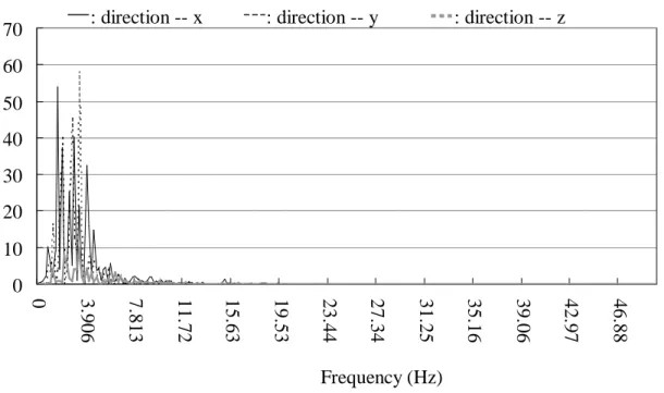
In this study, the proposed ECAM tracking scheme is used on the SP-120 simulator to simulate ground earthquake signal received at Shui-Li Primary School on September 21, 1998. Figure 12 shows a part of this ground earthquake signal. Figure 13 presents the power spectrum density of this signal at various frequencies. As aforementioned, the frequencies of the signal are not all less than one-tenth of the Nyquist frequency (here is 50 Hz). Nevertheless, poly-line curve-fitting method is used in the proposed control scheme.

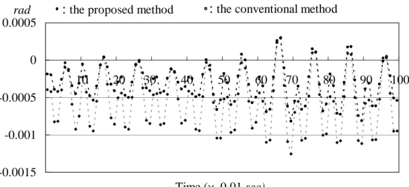
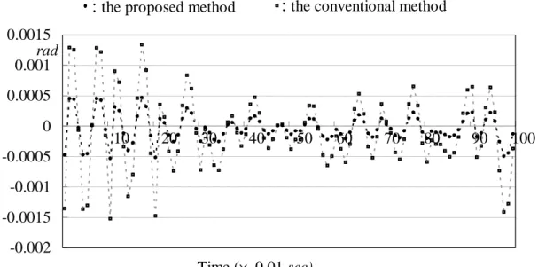
Figures 13 ~ 15 compare Euler’s roll angle errors, the pitch angle errors and the yaw angle errors, respectively, between the conventional and proposed method. This

ground earthquake signal involves only the translation; restated, the simulator’s output attitude must not include a rotational component. However as stated above, the six axes may mutually pull and drag each other, causing rotational motion during this pure translation. Table 3 presents the root mean square (RMS) errors of Eular angles for using the proposed ECAM tracking scheme and the master fixed ECAM tracking method executed on the simulator SP-120. In this simulation, the poly-line curve-fitting method is used to establish the ECAM profile and the positioning accuracy depends on the system sampling time: a smaller sampling time yields greater accuracy. However, a tradeoff exists between the calculation time and the system sampling frequency. For example, with a calculation time of around 0.5 ~ 1 ms, the system sampling frequency may be set to 100 Hz. Therefore, some small errors still occur (as shown in Figs. 14 ~ 16) even if the master switching tracking control is applied to the simulator system. Thus, higher performance computers clearly track more precisely.

四. 結論

The displacements of slaves of the electronic cam control system depend on the displacement of the master; the master switching method selects the most heavily loaded axis to be the master in real-time. The trajectory following speed yielded by the master switching method can be less than the speed yielded by the conventional (master fixed) method. Precision and robustness are the key concerns and the proposed method is sound. As aforementioned, by adjusting the proportional gain, a tradeoff exists between the robust stability and the velocity response of the control system. Using the well-known  analysis of structured uncertainty, a most appropriate proportional gain may be chosen to satisfy the demand of control performance, provided robust stability is guaranteed. Furthermore, the poly-line curve-fitting method requires less computational time than the polynomial curve-fitting method, although the latter one may theoretically yield higher precision for a motion of low frequencies.

Appendix A

To find the most heavily loaded axis of the six DOF motion simulator, SP-120, the Jaco bia n o f t he s imu lat o r sho u ld be calculated by the following procedure. A.1 Inverse Kinematics

Motion-based control may also be called cockpit’s positioning control. Cockpit position, including both translation and rotation components, must be transformed into the coordinates of the six sliders using inverse kinematics. The inverse kinematics of the SP-120 motion simulator is as follows.

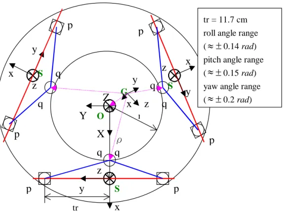
Figure 5 presents the top view of SP-120. 2 2 zi 2 yi yi 2 xi (q p ) q L q     (23) All of the parameters in Eq. (1) are fixed in the Si coordinate system. Thus,

} ] q q [q ) , , ( R ] Z Y [X { ) , , ( R ] [ T zi yi xi G T G G G zi yi xi T zi yi xi S S_{i i}          O O O i iq S (24) where R(,,) is the transformation matrix of the Euler angle, and can be easily expressed as,                                                c c s c c s c -c s -s s s -c s s s s c -c c ) , , ( R c s s s s c c s c (25) and c cos,s sin ,…. and so on, where the above variables and symbols are all presented in the nomenclature.

A.2 Jacobian formulation of simulator SP-12 From Eq. (23), 0 /d dq q )/d p d(q ) p (q /d dq q zi zi yi yi yi yi xi xi         t t t (26) 6 to 1 i , ] /d dq /d dq /d dq [ ] r r [r ] /d dq /d dq /d dq [ )] p /(q q 1 ) p /(q q [ /d dp T zi yi xi Si zi yi xi T zi yi xi Si yi yi xi yi yi xi yi        t t t t t t t (27) where, )] p /(q q 1 ) p /(q q [ ] r r [rxi yi zi  xi yi yi xi yi yi ; the superscript “T” represents the transpose

of the matrix and all the parameters are considered in the Si coordinate frame. From Eq. (24)

T G G G zi yi xi T zi yi xi Si ] d / dZ d / dY d / dX {[ ) , , ( ] /d dq /d dq /d dq [ t t t R t t t     } ] q q q [ ) d / d d / d / d ( T zi yi xi G t R t d R t R              (28) where R is the partial derivative of

) , , (  

R with respect to  . R_ is the partial derivative of R(,,) with respect to  . R_ is the partial derivative of

) , , (  

R with respect to  .

Substituting Eq. (26) into Eq. (25) yields

T G G G zi yi xi zi yi xi 1 6 yi ] d / dZ d / dY d / dX {[ ) , , ( ] r r [r ] /d dp [ t t t R t _      } ] q q q [ ) d / d d / d / d ( T zi yi xi G t R t d R t R              T G G G zi yi xi zi yi xi ] d / dZ d / dY d / dX {[ ) , , ( ] r r [r t t t R     } ] /dt d /dt, d /dt, d [ ] , , [    T    Qi R Qi R Qi  R (29) where Q_iG[q_xi q_yi q_zi]T. However,  ,  and  are the Euler angles measured in the body embedded coordinate frame, which is the cockpit coordinate system. When dealing with angular velocity, the inertial frame must be the reference frame. Let [xyz]T be the cockpit angular velocity measured in the inertial frame X-Y-Z-O. Then,

                                  t t t M t t t z y x /d d /d d /d d /d d /d d /d d c c s 0 c s -c 0 s 0 1 ] [ T                 (30) T 1 T ] [ ] /d d /d d /d d [  t  t  t M  xyz   (31) where, 1 1 ) ( c s -0 c s c c 0 s c -s s c   _                        c M (32)

Substituting Eq. (31) into Eq. (29) yields,

T G G G zi yi xi zi yi xi 1 6 yi ] d / dZ d / dY d / dX {[ ) , , ( ] r r [r ] /d dp [ t t t R t _      T 1 i i i, Q , Q ] [ ] Q [R_ R_ R_  M _x_y_z  (33)

According to the definition of Jacobian matrix J, the joint space is converted into Cartesian space, such that,

t J t X/d dΘ/d d   i (34) where X61[XG YG ZG α βγ]T , and yi i p  , i = 1 to 6, and t X J t d /d /d dΘ 1 i    (35) As mentioned above, the angular velocity in the inertial frame is more meaningful than that measured in the body embedded frame. Form Eq. (35), the elements of J1 can be

summarized directly as follows.

The first part of Eq. (35) comprises the first three columns of J1 ) , , ( ] r r [r ] [J_i₁1 J_i₂1 J_i₃1  _{xi yi zi} R_xi _yi _zi , i = 1 to 6 (36) The second part of Eq. (35) comprises the last three columns of 1

J ) , , ( ] r r [r ] [ xi yi zi xi yi zi 1 6 i 1 5 i 1 4 i J J R   J     1 i i i, Q , Q ] Q [       R_ R_ R_ M (37) A.3 Calculate the loaded torque of each joint using Jacobian matrix

The relationship between 6×1 joint torque vector ,  = 1, 2,3,4,5,6and the 6×1

equivalent Cartesian force-moment vector F,

F = m a, I3x3 acting at the mass center of

the upper plate, can be written in the form, (John, 1989)

 = J F. (38) T

References

Al-Muthairi N.F., Bingulac S., Zribi M., (2002). Identification of discrete-time MIMO systems using a class of observable canonical-form. Control Theory and Applications, IEE Proceedings, vol. 149, Issue: 2, March 2002, pp 125-130.

Chung I-Fang, Chang Hung-Hsiang & Lin Chin-Teng, (1999). Fuzzy Control of a Six-degree Motion Platform with Stability Analysis. IEEE International Conference on Systems, vol. 1, 1999, pp 325-330. Dierchx & Paul, (1993). Curve and Surface

Fitting with Splines. Oxford University Press.

Dixon R., Pike A.W., (2002). Application of condition monitoring to an electromechanical actuator: a parameter estimation based approach. Computing & Control Engineering Journal, vol. 13 Issue: 2, April 2002, pp 71-81.

Edwin K. P. Chong and Stanislaw H. ZAK, (1996). An Introduction to Optimization. A Wiley-Interscience Publication, John Wiley & Sons, INC., 1996, pp. 101-164. Garret N. Vanderplaats, (1984). Numerical

Optimization Techniques for Engineering Design: With Applications. McGraw-Hill Book Company, 1984.

John J. Craig, (1989). Introduction to Robotics Mechanics and Control – 2nd ed. Addison-Wesley Publishing Company, Inc., 1989, pp 211-215.

Kim Dean H. & Tsao Tsu-Chin, (2000). Robust Performance Control of Electrohydraulic Actuators for Electronic Cam Motion Generation. IEEE Transactions on Control Systems Technology, vol. 8, NO. 2, March 2000, pp 220-227.

Li-Shan Chen, (1995). Follower Motion Design in a Variable-Speed Cam System. Institute of Mechanical Engineering College of Engineering National Chiao Tung University, NCTU MEENG 1995, pt.11:3.

Plummer A.R., (1994). Non-linear control of a flight simulator motion system. Control Applications, Proceedings of the Third IEEE Conference on, vol.1, 1994, pp 365-370.

Reich, Jens-Georg, (1992). C curve fitting and modeling for scientists and engineers. New York McGraw-Hill.

Steven Chingyei Chung, (1995). The Tracking Control for The Electric Gear System. National Science Council of the Republic of China, NSC 845-012-011,

1995.

Werner H., (1996). Robust control of a laboratory flight simulator by non-dynamic multi-rate output feedback. Decision and Control, Proceedings of the 35th IEEE Conference on, vol.2, 1996, pp 1575-1580. Zhao qing-feng, (2000). Advanced Design for Automatic Control System: Using MATLAB Programming Langage. Chan Hwa Science and Technology Book Co., Chapter 6, Ltd, 2000, pp. 1-26.

Zhiwen Zhu, Leung H., (2002). Identification of linear systems driven by chaotic signals using nonlinear prediction. Circuits and Systems I: Fundamental Theory and Applications, IEEE Transactions on, vol. 49 Issue: 2, Feb. 2002, pp 170-180.

Zhou Kemin, (1998), Essentials of Robust Control. Prentice Hall, Inc., Upper Saddle River, New Jersey, 1998, pp. 55-62, pp. 129-211.

Calculate Jacobian Matrix J (Eq. (23) ~ Eq. (37)) m r, 1 , r ~y y

Calculate the heaviest loaded axis as the new master (Eq. 38) Establish cam profiles by using curve-fitting method: Polynomial curve-fitting method Eq. (17)~(23) or Poly-line curve-fitting method Eq. (24)~(28) Axis #1 Axis #2 Axis #3 Axis #4 Axis #5 Axis #m r,1 y r,2 y r,3 y r,4 y r,5 y m r, y Motion Planning Process

Fig. 1 Master switching method for m-axes ECAM control … … … 1 y 2 y

p

Fig. 2 Cam profile trajectory established using the polynomial curve-fitting method

Fig. 3 Cam profile trajectory established using the poly-line curve-fitting method

kT _{T (k+N) T}

The planned points

… … f(t) t VR t Cam profile kT _{(k+N) T} T

The planned points

… … f(t)

t

Fig. 4 Prototype SP-120

Fig. 5 Vertical view of the simulator platform SP-120 k S S S O ρ r

q

q

q

X

Y

Z

q

q

q

p

p

p

p

p

p

x

y

x

y

y

x

z

z

z

y

x

z













Fig. 6 Conditions on dual solutions using the polynomial curve-fitting method

Fig. 7 Equivalent model of slider

k t (k1)T ) ˆ ( _k1 m t f kT T k 1) (  ) ( _k m t f 1 ˆ_k t 0 ) ˆ ( ₁ ' _  k m t f m u c

Fig. 8 Simplified control system’s block diagram of control system of each slider of simulator SP-120

Fig. 9 Upper linear fractional transformation with ₁ _m, ₂ _c and |_m |1,|_c |1 1  matrix T _t r 2 G r y 1 G m  m  m / 1 +- 1 w 1 z s / 1 _1/s - 2 x x₁  x₂ y x1 c c fK K c E u f n K K / - + - + f a

K

K /

)

(

s

G

y

y

_z

Fig. 10 Singular value frequency responses, (G₁(j)), for various proportional gains, K _a

Fig. 11 Upper bounds of structured singular values, _(G₁(j)), for various proportional gains, K _a s rad / s rad / 0 . 12  a K 0 . 10  a K 0 . 5  a K 0 . 1  a K 0 . 12  a K 0 . 10  a K 0 . 5  a K 0 . 1  a K decreased as , increased || ) ( ||G₁ j _ K_a increased as , increased )) ( ( sup _{1 a} R K j G     )) ( ( ₁   G j )) ( ( ₁





Fig. 12 The piecewise ground earthquake signal involves only the translation.

Fig. 13 Power spectrum density of the ground earthquake signal at various frequencies -3 -2 -1 0 1 2 3 Time (× 0.01 sec) 10 20 30 40 50 60 70 80 90 100 direction -- x direction -- y direction -- z 2 / s m Ac ce ler ation 0 10 20 30 40 50 60 70 0 3. 906 7.813 11. 72 15. 63 19. 53 23. 44 27. 34 31. 25 35. 16 39. 06 42. 97 46. 88 Frequency (Hz)

Fig. 14 Comparison of Euler’s piecewise roll angle errors obtained using the proposed master switching method with those obtained the conventional method for ECAM control executed on the simulator SP-120

Fig. 15 Comparison of Euler’s piecewise pitch angle errors obtained using the proposed master switching method with those obtained the conventional method for ECAM control executed on the simulator SP-120

-0.0015 -0.001 -0.0005 0 0.0005 -0.01 -0.008 -0.006 -0.004 -0.002 0 0.002 Time (× 0.01 sec) Time (× 0.01 sec) rad rad 10 20 30 40 50 60 70 80 90 100 10 20 30 40 50 60 70 80 90 100

:

:

-0.002 -0.0015 -0.001 -0.0005 0 0.0005 0.001 0.0015

Fig. 16 Comparison of Euler’s piecewise yaw angle errors obtained using the proposed master switching method with those obtained using the conventional method for ECAM control executed on the simulator SP-120

rad

10 20 30 40 50 60 70 80 90 100

:

:

Table 1 Maximum singular values of G1(j) _, maximum structured singular values of )) ( ( sup 1  R  G j

and bandwidth of control system for various proportional gains, K ; the a

upper bound, m , of the nominal mass is set to 250 kg _H K _a terms 0.1 1.0 5.0 10.0 12.0  ) ( 1 j G 88.939455 18.651650 3.910155 2.323414 2.168739 )) ( ( sup ₁  R  G j 0.666652 0.666658 0.752879 0.929482 0.989907 Bandwidth (rad) 0.00594 0.0188 0.0420 0.0594 0.0651

Table 2 Critical upper bounds of the nominal mass for various proportional gains, K _a

a

K _{0.1 1.0 5.0 10.0 12.0} critical upper

bounds (kg)

10,400.0 1414.9 433.6 281.8 254.1

Table 3 Root mean square (RMS) errors of Euler angles, obtained using the proposed master switching method and the conventional method for ECAM control executed on the simulator SP-120 Error items Tracking method RMS error of roll RMS error of pitch RMS error of yaw

conventional method 0.0015150 rad 0.003427 rad 0.0004285 rad master switching

method