On Extracting Color-Size Features for Image Classification

On Extracting Color-Size Features for Image Classification

Cheng-Chieh Chiang

(江政杰), De-Wei Fu

(傅德瑋), Yi-Ping Hung

(洪一平),

Chiou-Shann Fuh

(傅楸善)

1. Department of Information and Computer Education,

National Taiwan Normal University, Taipei, Taiwan, R.O.C.

2. Department of Computer Science and Information Engineering,

National Taiwan University, Taipei, Taiwan, R.O.C.

Tel: (02)2362-5336 ext. 433, Fax: (02)2362-8167, e-mail: [email protected]

Abstract

Image classification based on low-level visual features is an important but challenging task for category indexing and learning in content-based image retrieval. To improve the performance of image classification, we propose a new type of features, called color-size features, which contain the distribution information of both color and region-size together. This paper considers two kinds of color-size features: color-size histogram and color-size moments, where the latter are a condensed version of the former but can achieve better classification results. An unavoidable step on extracting color-size features is to choose an appropriate method for image segmentation. Our experiments have shown that, by using the multi-scale watershed segmentation algorithm, the performance of image classification using color-size moments is significantly better than that of using color moments alone.

Keywords: color-size feature, feature extraction, image classification, watershed segmentation

1.Introduction

Image classification based on low-level visual features is an important issue in computer vision and image processing. Image classification is widely used for medical images, satellite images, content-based image retrieval (CBIR), etc. In CBIR, the category indexing can

be constructed by image classification such that people can use the semantic commands to retrieve the image data. Image classifiers extract low-level visual features from an image to make a decision which category the image belongs to. Therefore, the classification can build a bridge to connect the low level features and the semantic information in the image.

Extracting of visual features will be important because we can get them from images directly. Many types of visual features were proposed such as color, texture, shape, etc. This paper will focus on color features. Color is one of the most recognizable elements of image contents. Many types of color features are discussed: color histogram and color moments [8][9][10], color correlogram [4], and four kinds of color descriptors defined in MPEG-7 such as scalable color, dominant color, color layout, and color structure [7][14].

To improve the performance of image classification, we propose a new type of features, called color-size features, which contain the distribution information of both color and region-size together. To get the region-size information, it first needs to partition the images into a set of regions using an image segmentation method. We choose the watershed segmentation method [12][13] to partition the image into regions. In this paper, we will

consider two kinds of color-size features: color-size histogram and color-size moments. Color-size histogram is the distribution of pixels having attributes of color and region-size in an image. Therefore, color-size moments are moment computation from color-size histogram.

The paper is organized as follows. Section 2 reviews color features including color histogram and color moments, and then introduce the region-size features. In section 3, we will propose the details of color-size features, including color-size histogram and color-size moments. Then we will discuss the approach of image classification using color-size features in section 4. Section 5 will give the experimental results of proposed features. Our experiments will compare the classification results using different features by KNN classifier. Finally, conclusions and future works of this paper are shown in section 6.

2. Color Features and Region-size

Features

In this section, we first review color features, and then introduce the region-size features.

2.1. Color features

Color histogram can be used to represent the color distribution of colors in an image. To compute color histogram, a color space is first chosen, e.g. HSV, LAB, LUV, etc. By mapping the colors in an image into a discrete color space containing n colors, the color histogram can be expressed as a feature vector

CH = (h1, h2, …, hn)

where each element hi contains values in three color channels to represent the number of pixels of i-th bin in the image.

Choosing n is the quantization problem of

color bins. One way is to choose a fixed number. Lim and Leow [6] proposed an adaptive histogram approach which perform color clustering to decide the number of color bins. When n is small, the length of feature vectors is small and the computation is more efficient. However, the feature vectors are less accurate in representing the image.

Stricker and Orengo [9] used the central moments of each color channel to overcome the quantization effects in the color histogram. Color moments can characterize the color distribution. Let xi be the value of pixel x in i-th color

component, and N be the pixel number of the image. The first- and second-order color moments of an image can be defined as:

CM = {m1, m2, m3, s11, s22, s33} where

∑

₍

₎

∑

Color histogram and its derived color moments are simple and efficient features for image classification. They are insensitive to small changes in camera viewpoint. However, color histogram only captures the color distribution of images. It cannot represent other useful information contained in an image. Two images with similar color histogram may look quite different.

2.2. Region-size features

By using an image segmentation method, an image can be partitioned into a set of regions. We can assign a region-size attribute to each pixel, which is the size (or the pixel number) of the segmented region containing this pixel. Hence, the region-size distribution will contain the structure information of an image. Different images will have different region-size

distribution.

Any image segmentation method can be used to extract the region-size information. In this work we use the well known watershed segmentation [12][13] to partition an image into non-overlapping regions. Watershed segmentation is an efficient, automatic, and unsupervised segmentation method. Because the basic watershed algorithm is highly sensitive to gradient noise, so it usually results in over-segmentation.

To prevent the over-segmentation problem, a pre-processing method called “topographic simplification” proposed by [13] will be applied in our implementation. Two parameters, r and h, can be used to control the coarseness of the segmentation results. The parameter r is the size of the structure element of the dilation operation, and h is the height of elevation used in the erosion operation for eliminating the local minima. As r and h become larger, the number of regions generated decreases. The two parameters r and h are referred to as the scaling parameters because they can determine the number of regions generated by watershed segmentation. When the image size is m by n, the value of region-size can range from 1 to mn. To reduce the computation complexity, we quantize the value of region-size into s levels, where s << mn.

3. Proposed Color-size Features

By combining the color and region-size features, we can form a new type of color-size features. In this paper, we consider two kinds of color-size features: color-size histogram and color-size moments.

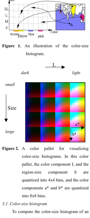
Figure 1. An illustration of the color-size

histogram.

L

Size

Figure 2. A color pallet for visualizing

color-size histograms. In this color pallet, the color component L and the region-size component S are quantized into 4x4 bins, and the color components a* and b* are quantized into 8x8 bins.

3.1. Color-size histogram

To compute the color-size histogram of an image, we need to first partition the image into a set of regions in order to acquire the region-size attribute for each pixel. Let K1, K2, and K3 be the

number of bins used for quantizing the three color attributes, and K4 be the number of bins for

the region-size attribute. Then, a color-size histogram (CSH) of an image is a K1 x K2 x K3 x

K4-dimensional feature set, i.e.,

CSH = { hijkl | 1≤i≤K1, 1≤j≤K2, 1≤k≤K3,

in which each hijkl of the histogram contains the

number of pixels having the attribute values of three color components, Li, aj*, bk*, and

region-size, sl.

In the following experiments, we adopt CIE LAB color space, and let K1=4, K2=8, K3=8,

and K4=4. Figure 1 illustrates the voting process

of extracting the color-size features. For example, pixel A of the image on right hand side has a blue color, and is contained in an extra-large (XL) region. Then the bin corresponding to the blue color and the XL region-size will be incremented by one.

Figure 2 shows a color pallet for visualizing color-size histograms. Figure 3 illustrates the difference between the traditional color histogram and the proposed color-size histogram. Here, (a) and (b) show two images and their corresponding color histograms. (c) and (d) show the segmentation results of the two images and their color-size histograms. All histograms are displayed based on the color pallet shown in figure 2. Notice that the color histograms of these two images are similar, but their color-size histograms are quite different, which implies the color-size histogram is more discriminative.

3.2. Color-size moments

As stated above, each pixel of an image has four attributes: three color components and one region-size. Let xi, i=1, 2, 3, 4, be the value

of pixel x in i-th color component (i is 1, 2, or 3) or region-size (i is 4), and N be the pixel number of the image. Color-size moments, with first and second order moments, of an image will be defined as: CSM = (m1, m2, m3, m4, s11, s22, s33, s44, s12, s13, s14, s23, s24, s34) where

∑

(

)

∑

(a)

(b)

(c)

(d)

Figure 3. An illustration of color histogram and

color-size histogram. (a) and (b) are original images and related color histogram. (c) and (d) are segmented images by setting r=1 and h=3, and their color-size histogram.

Notice that the color-size moments defined here is a much more compact feature set than the color-size histogram because it forms a 14-dimensional feature space while the color-size histograms shown in section 3.1 have 4x8x8x4=1024 dimensions.

4. Image Classification

Assume some semantic categories for image classification are pre-defined, and each test image will be classified into one category. i, j = 1, 2, 3, 4

image will be thought as consisting of several blobs, where each blob is coherent to color and texture space. Diligenti et. al. [3] introduced a structured representation of images based on labeled XY-trees. Then a probabilistic architecture was proposed to extend hidden Markov models for learning probability distributions defined on spaces labeled trees. Huang et. al. [5] provided a hierarchical image classification scheme. First the classification trees are constructed by the training data. Then the tree can be used to category new images. Vailaya et. al. [11] also built a hierarchical scheme to classify the vocation images into the categories of indoor or outdoor; outdoor images are classified as city or landscape; finally landscape images are classified as sunset, forest, and mountain classes. In [15], a one-dimensional hidden Markov model was provided for indoor/outdoor scene classification.

In our work, we want to show the performance using color-size features of image classification. To simplify the problem, we choose the KNN classifier and use Euclidean distance. KNN classifier is a simple, efficient, and non-parametric classification approach. For the problem of selecting training data, we adopt leave-one-out strategy in KNN classifier. Only one image of each category is tested each time, and the other images will be training samples. All images in the database will be tested if they are classified correctly or not. However, KNN classifier is a search problem of looking for the k closet samples from testing input. If the search space is huge, KNN classifier may be slow. We can use the fast algorithm [2] to improve the execution speed for nearest neighbor search.

ID=1 Glaciers and Mountains ID=2 Monument Valley ID=3

Autumn ID=4 Caverns

ID=5

Fireworks ID=6 Doors of Paris ID=7 Dolphins and Whales ID=8 Owls ID=9

Fitness ID=10 Prehistoric World ID=11 Bonsai and Penjing ID=12 Tropical Plants ID=13 Beautiful Roses ID=14 Museum Duck Decoys ID=15

Cuisine ID=16 Museum Easter Eggs

Table 1. The example images, category id, and

name of each category.

5. Experimental Results

We arbitrarily choose sixteen categories from Corel Photos and each category consists of 100 photo images in our image database. Table 1 lists the categories ID, semantic names, and example images of each category. These images contain a wide range of content such as scenery, animal, plant, etc. Now we will perform some experiments to compare the performance using size feature, color histogram (CH) vs. color-size histogram (CSH), and color moments (CM) vs. color-size moments (CSM).

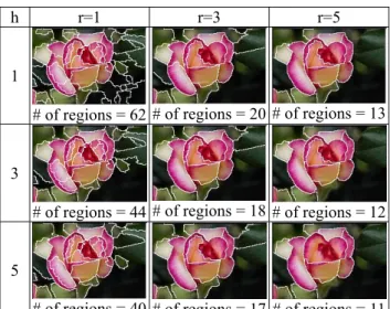
First we will consider the influence of scaling parameters, r and h, in watershed segmentation. Table 2 shows the changing of region numbers with different r and h. We can find that r is more important than h in controlling the segmentation results. In the following experiments, we will only consider parameters r in order to simplify the problems.

h r=1 r=3 r=5

1

# of regions = 62 # of regions = 20 # of regions = 13

3

# of regions = 44 # of regions = 18 # of regions = 12

5

# of regions = 40 # of regions = 17 # of regions = 11

Table 2. The watershed segmentation results

controlled by scaling parameters r and h k Size CH CSH CM CSM 1 50 73.1 75.5 75.8 83.8 5 51.3 73.4 75.8 77.9 83.8 9 51.8 71.8 75.7 76.9 82.6

Table 3. The recognition rates (%) using size

feature, CH: color histogram, CSH: color-size histogram, CM: color moments, and CSM: color-size moments.

Table 3 is the list of recognition accuracies using five kinds of features with different values k of KNN classifier. Here we use the scaling parameter r=1. The case of changing scaling parameter r will be discussed later. By table 3, the recognition rate is about 50% only using region-size feature. But using color-size features, combination of color and size features, are better than color features, either color-size histogram vs. color histogram or color-size moments vs. color moments. Moreover color-size moments have the highest rates in all cases of value k. Table 4 shows the list of classification rates only using color-size moments with changing scaling parameter r and k of KNN classifier. We can know that the classification rates will be kept well and stable using color-size moments with different r and k.

r=1 r=3 r=5 k=1 83.8 82.2 79.5 k=5 83.8 81.5 79.3 k=9 82.6 80.8 79.1

Table 4. The recognition rates using color-size

moments feature with changing r and k.

(a) color histogram vs. color-size histogram

(b) color moments vs. color-size moments

Figure 4. The recognition rate details of all

categories using different features with k=5 and r=1

Figure 4 shows the detail rates of each category in the setting of k=5 and r=1. We can find that color-size moments are better than color moments, and the difference between color histogram and color-size histogram are not obvious. Because color histogram is high dimension features, the additional region-size features cannot have better signification improvement. In the other hand, color moments are low dimension features, so the size feature is helpful for accuracy improvement.

Table 5 is the classified confusion matrix of all categories using color-size moments with k=5 and r=1. The titles of each row and column

are category id. Cells of the table are the number of testing results corresponding to the category id. The diagonal items with boldface in table 5 are numbers of correct assignments, and the others are fault assignments. For each category, there are 100 testing samples totally of each category. 1 2 3 4 5 6 7 8 9 10 11 12 13 14 15 16 1 82 2 2 0 0 1 0 0 2 0 5 1 0 3 0 2 2 8 83 0 1 0 0 3 1 1 0 1 0 0 0 0 2 3 8 7 73 2 0 1 0 0 0 0 4 4 1 0 0 0 4 0 1 4 84 0 2 3 0 0 0 2 0 2 0 2 0 5 1 0 1 4 86 0 0 5 0 0 1 1 0 0 1 0 6 0 1 3 4 0 86 0 0 2 0 2 1 0 0 1 0 7 2 0 0 0 1 0 90 0 0 0 5 0 0 1 0 1 8 4 3 4 4 3 0 0 80 0 0 0 1 0 0 0 1 9 0 0 0 0 0 0 0 0 93 4 0 0 0 1 0 2 10 0 0 0 0 0 0 0 0 5 91 0 0 0 4 0 0 11 5 0 1 1 0 0 3 0 0 0 83 1 0 4 2 0 12 1 0 14 0 0 0 0 1 1 0 4 70 5 0 3 1 13 1 0 4 3 2 1 0 2 0 0 0 5 78 0 4 0 14 0 0 0 0 0 0 0 0 2 6 1 0 0 91 0 0 15 0 2 9 6 0 1 0 0 0 0 1 5 1 0 75 0 16 1 1 0 0 0 0 0 0 1 0 0 0 0 2 0 95 Table 5. The confusion matrix of each

category using color-size moments with k=5, r=1

Because the sixteen categories are defined in the semantic view, some images are difficult to be classified. In fact, no features are always doing well in classification. The recognition accuracies using a feature will depend on the image contents. Figure 5 shows the illustrations of 2 categories, beautiful roses and tropical plants, where (a) to (c) are former and (d) to (f) are latter. Images (d), (e), (f) have similar color with (a), (b), (c) respectively. Images (a) and (b) are classified to tropical plants, i.e. misclassification, using color moments but correct using color-size moments. Image (c) is missed to tropical plants using both color moments and color-size moments. In the other words, size features are helpful to classify (a) and (b), not to (c). If we want to classify (c)

correctly, other reasonable features have to be used. From table 5, we can find some larger numbers of misclassification, e.g. there are 8 misses in both cases of that category 2 and 3 are classified to 1, 14 misses in that 12 to 3, and 9 misses in that 15 to 3. In fact, images of category 1, 2, 3, 12, 15 are easily confused because they contain sky, mountain, green background, colorful flowers, etc. Even in these confused categories, size features also improve the accuracies of image classification.

(a) (b)

(c)

(d) (e) (f)

Figure 5. Illustrations of category 13, Beautiful

Roses (a) to (c), and 12, Tropical Plants (d) to (f).

6. Conclusion and future work

This paper proposes the color-size features, including color-size histogram and color-size moments, to improvement the recognition performance of image classification. We have described the extraction process of color-size features and the image classification using color-size features. We also provide some experiments to compare the accuracies using color-size features in image classification.

For the future works, we will plan three directions to extend the color-size features. First, We want to design a scheme to include all scale information to be the multi-scale color-size features. Second, we will integrate the size feature into other features of images, such as texture, shape, etc. Moreover, we need to have

different features for different image contents in image classification. Finally, we will develop a CBIR system using the category indexing to provide the semantic concepts for users. The techniques of image classification will be helpful for category indexing construction and feedback scheme.

REFERENCES

[1] S. Belongie, C. Carson, H. Greenspan, and J. Malik, "Color- and texture-based image segmentation using EM and its application to content-based image retrieval", ICCV '98. [2] Y. S. Chen, Y. P. Hung, C. S. Fuh, “Fast

Algorithm for Nearest Neighbor Search Based on a Lower Bound Tree”, ICCV 2001: 446-453.

[3] M. Diligenti, P. Frasconi and M. Gori, “Hidden Tree Markov Models for Document Image Classification”, in Proceedings of the sixteenth International Conference on Document Analysis and Recognition, 2001, Page(s): 849-853.

[4] J. Huang, S. R. Kumar and M. Mitra, W. -J. Zhu, “Spatial Color Indexing and Applications”, ICCV 98.

[5] J. Huang, S. R. Kumar and R. Zabih, “An automatic hierarchical image classification scheme”, in Proceedings of the sixth ACM international conference on Multimedia, 1998, Pages 219 – 228.

[6] F. S. Lim, and W. K. Leow, “Adaptive Histogram and Dissimilarity Measure for Texture Retrieval and Classification”, in Proceedings of International Conference on Image Processing, 2002.

[7] S. Manjunath, J.-R. Ohm, V. V. Vasudevan, and A. Yamada, “Color and texture descriptors”, IEEE Transactions Circuits

Systems Video Technol (Special Issue on MPEG-7), 11(6), June 2001, pp.703-715. [8] J. Smith, Integrated Spatial and Feature

Image Systems: Retrieval, Compression and Analysis, Ph.D. thesis, Graduate School of Arts and Sciences, Columbia University, San Diego, CA, USA, 1997.

[9] M. Stricker and M. Orengo, “Similarity of Color Images”, in Proceedings of SPIE Storage and Retrieval for Image and Video Databases,1995, pp.381-392.

[10] M. J. Swain and D. H. Ballard. “Color indexing”, International Journal of Computer Vision, 7(1): 11-32, 1991

[11]A. Vailaya, M. A. T. Figueiredo, A. K. Jain, H. J. Zhang, “Image Classification for Content-based Indexing”, IEEE Transactions on Image Processing, Volume: 10 Issue: 1 , Jan. 2001 Page(s): 117 –130.

[12]L. Vincent and P. Soille, “Watersheds in digital spaces: an efficient algorithm based on immersion simulations”, IEEE Transactions on PAMI, 13(6), Jun. 1991, pp.583-598.

[13] D. Wang, “A Multiscale Gradient Algorithm for Image Segmentation Using Watersheds”. Pattern Recognition, 30(12):2043-2052, 1997.

[14] A. Yamada, et.al., “MPEG-7 Visual Part of Experimentation Mode Version 9.0”, ISO/IEC/JTC1/SC29/WG11/N3914, Jan. 2001.

[15] H. Yu and W. Wolf, “Scenic Classification Methods for Image and Video Databases”, SPIE International Conference on Digital Image Storage and Archiving System, 2606:363-371, 1995.