Maximum-likelihood-based filtering for attitude determination via GPS carrier phase

Maximum-Likelihood-Based Filtering for Attitude Determination

via

GPS

Carrier Phase

H.

M. Peng,

Y.

T. Chiang and

F.

R.

Chang

Department of Electrical Engineering

National Taiwan University, Taipei, Taiwan,

R.

0.

C.

L.

S.

Wang

Institute of Applied Mechanics

National Taiwan University, Taipei, Taiwan,

R.

0.

C.

ABSTRACT

In this paper, a maximum-likelihood-based (ML- based) filter is proposed for attitude determination via the GPS carrier phase observables. The quaternion rep- resentation is adopted here to describe the attitude. Hence, the norm constraint on the quaternion should be considered. The ML estimation with Lagrange multipli- ers can be used to consider simultaneously the evolution equation and the constraint, and to minimize the error covariance matrix. The attitude determination via GPS

carrier phase observables is fulfilled in two steps. The first step is the GPS carrier phase ambiguity resolution. After the integer ambiguities being fixed, the ML-based filter is used to determine the optimal attitude. The ad- vantage of adopting the quaternion as the state vector to describe the kinematic behaviors is that no singular problems arise.

To

verify our algorithm, the simulation has been conducted. In the simulation, the white noises are added on the carrier phase observables to assess the performance of the proposed method. The body frame is formed by three non-colinear GPS antennae which are mounted on a platform with two aluminum bars repre- senting the baseline vectors. According to the simula- tion, our method is sound and effective.

I INTRODUCTION

The problems of attitude determination frequently arise, such as in the navigation and control of vehicles, in the attitude determination and control of spacecrafts. The sun sensor, the horizon sensor, and the gyroscope are some popular sensors [20] to obtain the attitude in- formation. All these sensors have some defects, however. The sun sensor is invalid when the satellite is behind the Earth. Since the horizon of the Earth is poor de- fined, the accuracy of the horizon sensor is limited. The

drift problem, i.e., the accumulation of errors, associ- ated with the gyroscope makes it necessary to calibrate periodically. The advent of GPS provides another route to solve the problem of attitude determination. Accord- ing t o the system characteristics, GPS does not have any of the problems that plague the sensors mentioned above.

GPS is a satellite-based navigation system, and its applications includes the positioning, navigation, tracking, and surveying [7]. Considering the accuracy requirement of attitude determination, the GPS car- rier phase observables are the most adequate measure- ments. Based on the idea of interferometry, several ai- gorithms for attitude determination have been devel- oped in [2, 5 , lo]. The main difficulty of using car-

rier phase measurements is to find the initial ambigui- ties. This problem has been investigated by many re- searchers. Various methodologies have been proposed, such as the ambiguity search techniques [4, 10, 191, the ambiguity function methods [13, 211, and the triple-

difference methods [2, 141. The first two methods pro- cess the double differences of carrier phase observables. The integer ambiguity problem is solved by search algo- rithms either on the space of possible ambiguous values

or on the space of possible coordinates. The triple- difference methods including the space-difference and time-difference algorithm eliminate the ambiguities t o calculate the coordinates. In this paper, the ambiguity function method is used t o estimate the carrier phase integer ambiguities.

On the other hand, an appropriate algorithm for determining the attitude is also essential, which affects the computation efficiency and the accuracy of the at- titude determination. The problem of attitude deter- mination is to find an orthogonal matrix, also called as the attitude matrix, which can be used to represent the rotational relationship between the vectors measured in

the reference frame and in the body frame. The atti- tude matrix has several representations [17], such as the nine components in a 3 x 3 rotation matrix, the Eulerian

angles, and the Euler-Rodrigues symmetric parameters (also known as the quaternions). The rotation matrix is the most natural representation, but the orthogonal property is difficult to retain. The Eulerian angles are 3-degree-of-freedom minimal representation without any constraint. However, the singularity may occur at some specific angles. The quaternion represents the attitude by four parameters with one constraint. The QUEST al-

gorithm [18] is one typical approach to solve the attitude determination problem, but it is suitable for single epoch only. Considering the vector measurements at different epochs, some modified algorithms are proposed in the literature, such as the filter QUEST method [15], the REQUEST algorithm [l], the extended Kalman filter method [8, 161, and the H , filter method [ll]. The first two methods are upgraded from the QUEST algorithm, but they can not handle the process noise. Using quater- nion as the state variables, the latter two approaches can tackle the process noise and the measurement noise. However, the norm constraint of quaternion is resolved by the dimensional reduction of the state variables. A more typical approach is to consider the evolution equa- tion of the quaternion and the norm constraint equation together. In other words, the differential equation and the algebraic constraint are dealt with simultaneously. In this paper, a maximum-likelihood-based filtering with Lagrange multipliers is adopted for considering such a singular system.

To verify our algorithms, the simulation has been conducted. The simulation is used to assess the per- formance of the proposed method. Three non-colinear antennae are assumed to be mounted on a two-degree-of- freedom platform with two aluminum bars representing the baseline vectors. By processing the generated car- rier phase observables with white noises from the three antennae attached to the ends of the bars, the proposed filter can be used to estimate the attitude. The sim- ulation shows that the proposed method is sound and effective.

This paper is organized as follows. In section 11,

the GPS carrier phase double-difference model is briefly described. The ambiguity function method is also dis- cussed in this section. In section 111, the concept of ML estimation with Lagrange multipliers is discussed. The application to attitude determination is introduced in section IV. The simulation is discussed in section V. Conclusions are given in section VI.

I1

GPS CARRIER

PHASE

MODEL

The GPS carrier phase observable counts the beat phase, i.e., the difference between the L-band carrier wave from a satellite and the reference signal generated by the receiver. It can be modeled as [6]

@

A = $A

+

c(6tj

-

6 t A )

+

_-

_diOn

+

_dirop

+

_E;,

₍₁₎

where

@

;

is the carrier phase measurements of the re- ceiver A from the j-th GPS satellite;

$*

is the true distance between the receiver A and the j-th GPS satel- lite; c is the speed of light; 6t3 and 6 t A are the clock

biases of the j-th satellite and the receiver A, respec- tively; X is the GPS carrier wavelength; N denotes the initial phase integer ambiguity; and diOn

,

dirOp

,

9;

and are the ionospheric delay, the tropospheric delay and the unmodelled errors, respectively. The units of all the terms in the equation are meters.

To eliminate the biases and the errors from satel- lites and receivers, it is customary to perform double differences between two receivers and two satellites. De-

noting the two receivers as A and B and the satellites as j and IC, the double-difference equation is

(2)

@'k A B

-

-

p

A B

+

XNi; f

where the convention

*cB

= (*:

-

) *:

-

(*;

-

);* is used, and the asterisk may be replaced by

4

,

p

,

N and

E . The satellite clock bias, the receiver clock bias, the

ionospheric delay, and the tropospheric delay are then eliminated in the double-difference model.

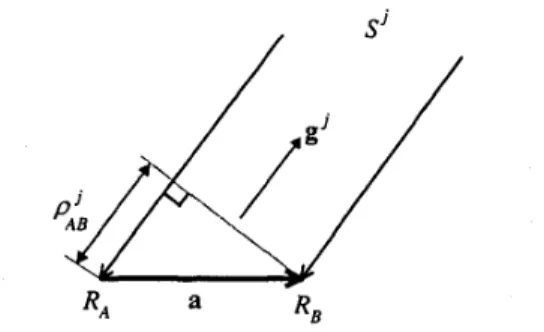
The concept of interferometry is described in the following. In Figure 1, R A and RB denote two GPS antennae which are mounted on the two ends of base- line vector a, respectively. They receive signals from the same GPS satellite denoted as

Si

with the same unit directional vector gj. The difference between the distances from the two antennae to the satellite S j is then

where the superscript T denotes the transpose.

With n satellites (n >_ 4) being observed at the same time, the matrix form of the equations can be writ- ten from (2) and (3) as

P A B = (&)'a, (3)

4? = STa

+

AN

+

E, (4)

where

s

=

[

51 s2

...

sn-1

3

4? =

[ 4fi2B

4yB

* . -

4i%

1''

=

[

g2 -g' g3 -gl

...

gn -gl

3 ,

N =

[

N+& N i &

N G

I T ,

, S'

Figure 1: Concept of interferometry method

The main difficulty in using this model is on the de- termination of the initial integer ambiguities N. In the following discussion, the ambiguity function method is briefly described for estimating the integer ambiguities. Assuming that the position of the receiver A is known and n satellites are observed. The coordinates of re-

ceiver B (PE) are the unknown parameters. Consider the ambiguity function defined below

n

Note that the argument of the cosine function is the dif- ference between the double-difference phase observable and the double-difference true range multiplied by

F.

Comparing with (2), this term is equal to the double- difference ambiguity multiplied by 2a. Hence, if the correct coordinates PE are substituted into the ambigu- ity function, the function F should be maximized. Ac- cording to the above statements, the ambiguity function method can be divided into three parts. The first step is the computation of an approximation PE, which can be achieved by the DGPS algorithm, or the triple dif- ference method. Next, the candidates generated by the grid points surrounding the approximation p~ are sub- stituted into the ambiguity function. The maximizer is the optimal estimate p ~ . The final step is to determine the integer double-difference ambiguities, which can be computed from (4).

I11

INTRODUCTION

TO

ML-BASED

FILTERING

In this section, a maximum-likelihood-based (ML-

based) filtering is described. The derivation of the ML-

based filtering was proposed in [12], and the results are presented here for completeness. If the considered sys- tem is nonlinear and the extra constraint exists, the linearized system based on the Taylor series expansion

with constraint is used in the proposed method. Since the constraint equation may not be linear, the final es- timate may be found by iterations.

According to the lemmas proved in [12], it has been shown that previously processed measurements can be included in the form of a aggregated measurement for the variables that have been estimated and the irrele- vant variables can be discarded. It constitutes the basis

of the recursive procedure of maximum likelihood esti- mates. Based on the above discussion, the linear ML-

based filtering can be derived as follows. Considering the following discrete system equation and measurement equation

x k + l = A k X k -k w k , (6) Y k = C k X k + V k , (7)

where V k and W k are zero-mean independent Gaussian

noises with covariance matrices R k and Q k , respec-

tively. Let P k denote the error covariance associated

with the filtered estimate ? k , with %O and P O given by

the prior distribution for X O . %k+l and P k + l are, re-

spectively, equal to the maximum likelihood estimate of x k + l and its associated estimation error covariance

based on the following observations

Y k + l = C k + l X k + l -k v k + l , (8)

A k g k = x k + l

+

A k r k

-

w k , (9)

where the aggregated measurement ?k = X k + r k is used

to substitute for the prior measurement of X k , in which r k is a Gaussian random vector, independent of w k , with

zero mean and variance P k . Furthermore, the filtered

estimate 12k+l and the corresponding error covariance

P k + l can be obtained from the following recursions: ?k+l =

[

0 0 1

]

[ A k p k t T + Q k R k f l 0 c k + l ] I 4- [.;I] A k a k

,(lo)

CZ+I 0

P k + l = - [ 0 0 I ]

[ A k p k t r + Q k R k + l 0

c:+l]

4-

[

H]

> (11) where 2 means the estimate of x and the superscript

+

represents the pseudo-inverse [3, 91. If this matrix is invertible, the pseudo-inverse is equivalent to the inverse operation.

If the considered system is nonlinear, and some ex- tra constraints are exist, the linearized system based on the Taylor series expansion with constraint is adopted

in the proposed method. Assuming that the nonlinear system with constraint equation is modeled as

x k + l = f k ( x k )

+

g k ( x k ) w k , (12) Y k + 1 = h k + l ( x k + l )

+

v k + l (13)

0 = I k + l ( X k + l ) (14)

The nonlinear function f k , g k r h k + l , and 1 k + l , if suffi-

ciently smooth, can be expanded in Taylor series about f k and ki+l as

f k ( x k ) = f k ( 2 k )

+

F k ( ~ k

-

&)

+

g k ( x k ) = g k ( f k ) + - . * = G k + * * *

h k + i ( X k + i ) = hk+i(f;+I)

+

H k + i ( ~ k + i -?;+I)

+

0 = I k + l

(fF+l)

+

L k + l ( X k + l

-

f;+l)

+

*

,

where f;+l = f k ( & ) . Neglecting higher order terms enables us to approximate the model (12), (13) and (14) as

X k + i = F k X k

+

G k W k

+

Uk (15)

Y k + l = H k + l X k + l

+

Vk+l

+

P k + l , (16)

0 = L k + l X k + l + Z k + l , (17)

where uk, pk+l, and z k + l are calculated on line from equations

~k = f k ( f k ) - F k f k (18)

P k + l = h k + l (fF+1)

-

Hk+lkL+l (19)

Z k + i = I k + l (fL+l)

-

L k + l f k + l . (20)

Thus, the estimate &+I and the corresponding covari- ance matrix P k + l are

& + 1 = [ 0 0 0 I ] F ~ P ~ F :

+

G ~ Q ~ G :

o

0 0 0 L k + l HZ+l L Z + I 0 0 0

[

I

r

~ ~

1

k ~ + ~ ~ Y k + l

-

Pk+l

I

-z;+1

1

'

P k + l = - [ 0 0 0 I ] F ~ P ~ F ;

+

G ~ Q ~ G :

o

0 0 0 L k + l HZ+l LZ+l 0 0 0 I

rei

After the estimate fk+l is computed, it can be used to substitute for 12;+l, and the linearization process with respect to may be conducted again. The conver- gent estimate &+I is the final solution.

IV

APPLICATION

TO

ATTITUDE

DETERMINATION

For applying the ML-based filter for attitude deter- mination, the attitude kinematics and the sensor mea- surements are described as follows.

Attitude Kinematics

In the following discussion, the attitude matrix is represented by the quaternion. The quaternion

ii

r e p resenting a rotation is defined as

L

94

J

where n is a unit vector represents the axis of rotation;

6 is the angle of rotation about the axis n. The nor-

malized quaternion will be denoted by an overbar. The quaternion possesses three degrees of freedom and sat- isfies the constraint

-T-

-

1

9 q -

The attitude matrix is obtained from the quaternion according to the relation [17]

= (Iq4I2

-

I9l2)I

+

29qT

+

244[1911, (24) where I is the 3 x 3 identity matrix and [Iql] is the anti- symmetric matrix defined as

[Isll

=

[

-43 O

!

;:I.

92 -91 0

This notation will be used generally for any 3 x 3 anti- symmetric matrix generated from a three-vector. The attitude matrix defined above transforms the coordi- nates of vectors in the reference frame to those in the body frame.

The kinematic relation between the attitude repre- sentation and the angular velocity can be found [20] to be (25) 1 %) d t = Z " ( W ( t ) ) ' i ( t ) , where

r

o

w3 -w2 w1

1

L

- w 1 -w2 -w3

o

J

and w = [ w1 w:! w3 ] denotes the angular velocity of the transformation. The equation (25) can also be written as

where

r

44 -43 42

1

L

-41 -42 -43

J

Assuming that the angular velocity can be modeled as

w = wk

+

E,, where E, is the zero-mean Gaussian white

noise with covariance matrix P,, the continuous-time state equation of the attitude is given by

(29)

d - 1

-q =

-n(wk)q

+

dt 2

According to (29), the discrete-time model can be writ- ten as

q k + l

= 7 ( t k + l y t k ) q k

+

vk. (30)

If the angular velocity w k is constant from time tk t o

t k + l , the state transition matrix 7 ( t k + l , t k ) can be writ-

ten as

Sensor M e a s u r e m e n t s

The attitude sensor measurements considered here are GPS carrier phase observables. In the following discussion, it is assumed that integer ambiguities have been solved and the phase observables are ambiguity- free. Based on the discussion in section 11, the relation between the, double-difference ambiguity-free phase ob- servables !@: and the attitude A is (cf.(4))

! @ Q ( t k ) = bTA(q(tk))sj

+

4 ( t k ) , (32)

where the vector bi is the i-th baseline vector repre-

sented in the body coordinate system; sj equals to the difference between directional vector gj+l and g1 repre-

sented in the reference coordinate system; !@: is the cor- responding double-difference ambiguity-free phase mea- surements; the error vector w: is the white noise with distribution N ( 0 ,

R:).

Based on (32), since

bTA(q)sj = Tr(A(q) (B{)*), ₍₃₃₎

where

Tr

denotes the trace operation and the matrix

B

is given by

Substituting (24) into (33), we have

Bij = bi(Sj)=.

bTA(q)sj = (42

-

qqT)'IkB;

+

2'Ik(qqTBs) +244~([lqllB;).

Introducing the quantities ~ i j= 'IkBjj = brsj,

Sij = B . . + B T i j

-

-

bi(Sj)=

+

sib:, Z i j = bi x s',

leads to the bilinear form

bTA(q)d =

qTKijq,

where the 4 x 4 matrix Kij is defined by

Thus, the sensor measurement equation (32) can be sim- plified as

Assuming that there are m baseline vectors and n

satellites, the matrix form measurement equation can

be written as

Attitude Determination

b y

ML- based Filter

From the above discussion, it is shown that the measurement equation is nonlinear. In the following, the estimate of quaternion and the corresponding CO- variance matrix will be derived by the ML-based filter- ing.

According to the quaternion norm constraint and

the equations (30) and (41), the linearized equations can be written as

-

%+l = * ( t k + l ) =

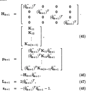
where (45)

(Gi+

1

1

% 2 G i + l Pk+l =

1

(Gi+l)TKm(n-l)Gi+i

J

--Hk+l%+l, (46) Lk+l =

qGi+$-,

(47) Z k + l = -(G;+1)%;+1

-

1. (48)

..-

According to (21) and (22), the filtered estimate

;Ik+l

and the corresponding covariance matrix Pk+l can be computed. For satisfying the nonlinear constraint equation, &.+l is being substituted for

Gi+l

until the

convergent &+I is found. The convergent condition is

the 1% norm error, while the normalization is performed to satisfy the constraint in the next iteration.

-

V

THE

SIMULATION

To verify our filtering algorithm, the simulation has been conducted. In the simulation, the white noise was added on the carrier phase observables for assessing the performance of the proposed method while the platform being rotated. Three non-colinear antennae were as- sumed to get the

GPS

satellites' signals and could form two baseline vectors for attitude determination. Note that the carrier phase integer ambiguities were com- puted by the ambiguity function method, hence, the carrier phase observables are all ambiguity-free.

The configuration of the simulation is described be- low. Two aluminum bars with three antennae mounted at the ends was used to represent two baseline vec- tors. The configuration of the two baseline vectors are shown in Figure 2. According to the figure, the representation of bl in the body coordinate sys-

tem was 5.885[ 1 0 ] and the representation of bz is 2.99[ cos(19.3472') sin(19.3472") 0

1.

These two aluminum bars were fixed on a rotation platform, which could be rotated by the AC servomotor.

The simulation is described as follows. The satel- lites ephemerides of PRN 1, 6, 14, 21, 22,25, 29,30 were

0

2.99 m 3.22 m

1.15 m

b, 5.885 m

Figure 2: Configuration of three antennae for simulation

and kinematic experiment

received by GPS receivers for computing the satellites' positions. The platform was assumed to be rotated with

a constant rate -0.0307 rad/sec. The initial attitude matrix was given as

1

0.4512 0.7282 -0.5159

A i n i =

[

-0.6554 -0.1221 -0.7454

.

-0.6057 0.6744 0.4221

Based on the above parameters, the phase observables can be generated for the simulation. The simulation time was 200 seconds. The white noise N(0, (0.0C1)~) is added on the phase measurements to assess the perfor- mance of the proposed algorithm. The generated phase measurements are shown in Figures 3 and 4.

b, double-difference phase observables

8 6 5 4 t

jj2

e o

$

-2

4

8-4 50 100 150 time (second)

Figure 3: bl double-difference phase observables in sim- ulation

The filtered attitude matrix computed by the proposed method and the unfiltered attitude calculated by the QUEST algorithm via the measurement of a single epoch is then transferred to yaw, roll, pitch angles, which are shown in Figures 5, 6, and 7. The expres- sions for these rotation angles in terms of the elements of the attitude matrix A are [20]

b, double-difference phase observables

5

-5

‘

J

50 100 150 200

time (second)

Figure 4: b2 double-difference phase observables in sim- ulation

yaw =

-

arctan(Aal /A22) roll =

-

arctan(A13/A33).

From the simulation results, it C&I be shown that the

proposed method can be used to determine attitudes in the kinematic case.

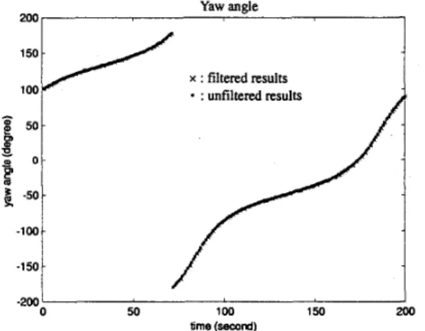
Yaw angle 200 - x : filtered results

-

: unfiltered results

t

5 0 -

0

O - e.

r

- 5 0 - - l o o r I 100 150 200 -200‘ 50 time (second)

Figure 5: Yaw angle of attitude matrix in simulation

VI

CONCLUSION

This paper is concentrated on attitude determina- tion via GPS carrier phase observables. Two main issues are considered in this topic. The first part is the ambi- guity resolution, while the ambiguity function method is adopted to resolve cycle ambiguities. The second part

is the algorithm for attitude determination. Based on

Roll angle 60 x : filtered results

-

: unfiltered results

/I

40 I 50 100 150 M O time (second)

Figure 6: Roll angle of attitude matrix in simulation

Pitch angle

80

c:

I

50 100 150 200

time (second)

Figure 7: Pitch angle of attitude matrix in simulation

the concept of maximum-likelihood estimation, the ML-

based filtering using GPS carrier phase measurements

for attitude determination has been studied. Some pre- liminaries about the maximum likelihood estimation are reviewed. The nonlinear constraints on state variable are also considered. This algorithm can be used to es- timate the state variable with some specific constraint equation.

If

the considered system is nonlinear, the lin- earized model is used. Comparing with the application in attitude determination, the norm of quaternion is the constraint equation. The sensor measurements observed from GPS are also nonlinear functions with respect to state variable, quaternion. For verifying the proposed algorithm, the simulation has been conducted. The sim- ulation can be used t o assess the performance of the pro- posed algorithm. The simulation results showed that the filtered results were smoother than the unfiltered results which were directly computed by GPS at every epoch.

References

[l] I. Y. Bar-Itzhack. Request, a recursive quest algorithm for sequential attitude determination.

Journal of Guidance, Control, and Dynamics,

19(5): 1034-1038,1996.

[2] R. Brown and P. Ward. A gps receiver with built- in precision pointing capability. In .IEEE Position

Location and Navigation Symposium, pages 83-93,

Las Vegas, Nevada, March 1990.

[3] S. L. Campbell and C. D. Meyer. Generalized In-

verse of Linear Transformations. Pitman, London,

1979.

[4] Dingsheng Chen. Development of a Fast Ambigu- ity Search Filtering (FASF) Method for GPS Car-

rier Phase Ambiguity Resolution. PhD thesis, The

University of Calgary, Calgary, Alberta, December 1994.

[5] Clark Emerson Cohen. Attitude Determination Us-

ing GPS: Development of an All Solid-state Guid-

-ance, Navigation, and Control Sensor for Air and Space Vehicles Based on the Global Positioning

System. PhD thesis, Stanford University, December

1992.

[6] Bernhard Hofmann-Wellenhof, Herbert Lichteneg- ger, and James Collins. Global Positioning System

Theory and Practice. Springer-Verlag Wien, New

York, fourth revised edition, 1997.

[7] Elliott D. Kaplan, editor. Understanding GPS:

Principles and Applications. Artech House, Boston

London, 1996.

[8] E. J . Lefferts, F. L. Markley, and M. D. Shus- ter. Kalman filtering for spacecraft attitude estima- tion. Journal of Guidance, Control and Dynamics,

5(5):417-429, September-October 1982.

[9]

S.

J

Leon. Linear Algebra with Applications.

Macmillan College Publishing Company, fourth edition, 1994.

[lo] Gang Lu. Development of a GPS Multi-Antenna

System for Attitude Determination. PhD thesis,

The University of Calgary, Calgary, Alberta, Jan- uary 1995.

[ll] F. L. Markley, N. Berman, and U. Shaked. Deter- ministic ekf-like estimator for spacecraft attitude estimation. In Proceedings of the American Con-

trol Conference, pages 247-251, Baltimore, Mary-

land, June 1994.

[12] Ramine Nikoukhah, Alan S. Willsky, and Bernard C. Levy. Kalman filtering and riccati equations for descriptor systems. IEEE Tran- sations on Automatic Control, 37(9):1325-1342,

September 1992.

[13] B. W. Remondi. Using the Global Positioning Sys- tem (GPS) Phase Observable f o r Relative Geodesy:

Modelling, Processing, and Results. PhD thesis,

University of Texas, Austin, May 1984.

[14] B. W. Remondi. Performing centimeter-level sur-

veys in seconds with gps carrier phase: Initial re- sults. In Proceedings of the Fourth International

Geodetic Symposium on Satellite Positioning, pages

1229-1249, Austin, Texas, April 1986.

[15] M. D. Shuster. A simple kalman filter and smoother for spacecraft attitude. Journal of the Astronautical Sciences, 37(1):88-106, 1989.

[16] M. D. Shuster. Kalman filtering of spacecraft atti- tude and the quest model. Journal of the Astro-

nautical Sciences, 38(3):377-393, July-September

1990.

[17] M. D. Shuster. Survey of attitude representations.

Journal of the Astronautical Sciences, pages 439- 517, October 1993.

[18] M. D. Shuster and S. D. Oh. Three-axis attitude determination from vector observations. Journal

of Guidance, Control and Dynamics, 4( 1):70-77,

January-February 1981.

[19] P. J . G. Teunissen. The least-square ambiguity decorrelation adjustment: A method for fast gps integer ambiguity estimation. Journal of Geodesy,

70(1-2):65-82, 1995.

[20] James R. Wertz, editor. Spacecraft Attitude Deter-

mination and Control. Kluwer Academic Publish-

ers, 1978.

[21] Joz Wu and Fong-Gee Yiu. Cosine functions of g p s

carrier phases for parameter estimation. Journal

of Surveying Engineering, 123(3):113-125, August