Efficient VLSI Architecture Designs for Shape-Adaptive DWT and Zero Tree Coding

全文

(1)Cover Page 1.. Workshop on multimedia technologies. 2.. Efficient VLSI Architecture Designs for Shape-Adaptive DWT and Zero Tree Coding. 3.. Short abstract In this paper, an efficient algorithm and its VLSI architecture design for a progressive still image coding system are presented. The image transform is a shape adaptive discrete wavelet transform (SA-DWT) using lifting scheme. The transformed image is then compressed by a shape adaptive zero tree coding scheme (SA-ZTC) in a progressive manner. The simulation results indicate the proposed SA-ZTC scheme enjoys a 4dB PSNR performance edge over the SPHIT algorithm under given bit rates. Combining both SA-DWT and SA-ZTC schemes, an efficient VLSI design was accomplished using the TSMC 0.35um 1P4M process. The post layout simulation results show that the chip is capable of working at above 60MHZ clock rate. The computing power implies a sustained processing rate of 42 frames/sec for 1024×1024 images.. 4.. 黃穎聰 Yin-Tsung Hwang and 王旭昇 Shi-Shen Wang 雲林科技大學電子系. 雲林縣斗六市大學路三段一二三號. Department of Electronic Engineering, national Yunlin University of Science & Technology 123 sec. 3, University Road, Touliu, Yunlin 640 e-mail: hwangyt@pine.yuntech.edu.tw Fax: 05-5312063 5.. contact author: 黃穎聰 Yin-Tsung Hwang. 6.. key words: texture coding, discrete wavelet transform, zero tree coding, shape adaptive, MPEG-4, VLSI design.

(2) Efficient VLSI Architecture Designs for Shape-Adaptive DWT and Zero Tree Coding Yin-Tsung Hwang, Shi-Shen Wang Dept. of Electronic Engineering, National Yunlin University of Science and Technology Toulin, Yunlin 640, Taiwan, ROC. ABSTRACT In this paper, an efficient algorithm and its VLSI architecture design for a progressive still image coding system are presented. The image transform is a shape adaptive discrete wavelet transform (SA-DWT) using lifting scheme and Daubechies (9,7) bi-orthogonal filters. The transformed image is then compressed by a shape adaptive zero tree coding scheme (SA-ZTC) in a progressive manner. For the SA-DWT design, we have successfully incorporated the shape information into the lifting DWT scheme so that redundant computations for the pixels outside of the shape can be eliminated. The proposed design can perform 1-D forward and inverse length adaptive DWT efficiently. The boundary extension problem, encountered in the lifting scheme and further complicated by the shape adaptive processing, was also resolved with minimum circuitry overhead. The 2-D SA-DWT is obtained by direct row-column operations of 1-D length adaptive DWT. For the zero tree coding design, we adopt the same 4-symbol coding system as suggested in the SPHIT algorithm. The coding scheme, however, is different and can support both shape adaptive and progressive coding. The simulation results indicate the proposed SA-ZTC scheme enjoys a 4dB PSNR performance edge over the SPHIT algorithm under given bit rates. The proposed scheme also facilitates efficient hardware design while the SPHIT algorithm is generally considered as too complicated to be implemented in hardware. Combining both SA-DWT and SA-ZTC schemes, an efficient VLSI design was accomplished using the TSMC 0.35um 1P4M process. The post layout simulation results show that the chip is capable of working at above 60MHZ clock rate. The computing power implies a sustained processing rate of 42 frames/sec for 1024×1024 images.. 1. INTRODUCTION Discrete Wavelet Transform (DWT) has been widely adopted in various visual coding applications such as JPEG2000 and the still texture coding in MPEG-4. It can achieve better compression performance at low bit-rate when compared with the block-based approach such as discrete cosine transform (DCT). Since MPEG-4 uses an object based coding, a shape adaptive DWT (SA-DWT), capable of processing only information within an arbitrarily shaped video.

(3) object, is required. The main distinction between an SA-DWT and a conventional-DWT lies in the capability of handling continuous short line segments encountered in a video object and the ability of resolving the complicated boundary extension problem efficiently. After SA-DWT, the derived coefficients are then quantized and coded to achieve data compression. Among various wavelet coefficients coding scheme such as vector quantization (VQ), trellis code quantization (TCQ), zero tree coding (ZTC) is the most popular one. Similarly, a shape-adaptive ZTC (SA-ZTC) is needed to process the outcomes of SA-DWT so that no information outside of the video object’s shape boundary is encoded to obtain high coding efficiency. In this paper, we will examine both SA-DWT and SA-ZTC modules from algorithmic and architectural aspects and present an efficient VLSI design with high coding efficiency. In the past few years, numerous studies [1-3] on the VLSI realizations of wavelet transforms have been reported. The architectures, mostly non-shape-adaptive, range from convolution, lattice structure to the latest lifting scheme structure. The lifting scheme was first proposed in [4], which constructs bi-orthogonal wavelets in the space domain. Compared with the classical Fourier based construction, the lifting scheme exhibits a much lower computing complexity and has been adopted widely these days. Recently, few papers [5,6] have begun to work on SA-DWT design. The designs emphasize on the shared 1-D structure for both forward and inverse transforms and on the resolution to boundary extension problem. As for the zero tree coding, various schemes using either scalar-based quantization or vector-based quantization have been developed. Although the wavelet vector quantization (WVQ) based approaches are feasible for real time processing, the corresponding hardware design complexity is prohibitively high. The scalar quantization based approaches, such as the well-known embedded zerotree wavelet (EZW) algorithm [7], and the set partitioning in hierarchical trees (SPIHT) algorithm [8], usually achieve good coding efficiency. The reported hardware designs, such as [9] for EZW, are non-shape adaptive. So far, no hardware realization for the shape-adaptive SPHIT algorithm has been proposed. The remaining of the paper is organized as follows. In Section 2, the lifting DWT algorithm and the proposed scheme for solving boundary extension problem are described. Section 3 presents our shared architecture design of 1-D lifting SA-DWT for both forward and inverse transforms. The proposed SA-ZTC algorithm is described in section 4. Section 5 describes the hardware design of the SA-ZTC. The performance simulation results of the combined SA-DWT and SA-ZTC are given in Section 6. Finally, the VLSI implementation results for the SA-DWT are given in section 7..

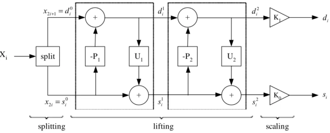
(4) 2. THE SHAPE-ADAPTIVE LIFTING DWT SCHEME In lifting scheme, the polyphase matrix of a wavelet filter is factorized into a sequence of alternating upper and lower triangular matrices and a diagonal matrix with constants. Each decomposed stage, called a lifting step, correspond to a simple filtering. In addition to the reduction in computing complexity, the lifting scheme also eliminates the need of explicit up-sampling and down sampling operations when compared with the traditional approach. Figure 1 shows the three major stages in the lifting scheme, i.e. splitting, lifting and scaling. In the splitting stage, input samples x(n) are split into two disjoint sets, called polyphase components. One correspond to the even indexed samples xe and the other correspond to the odd indexed samples xo . The lifting stage consists of several lifting step each containing a predict operator Pi and an update operator U i . The predict operator Pi estimates xo from xe and then produces a wavelet coefficient d i . The update operator U i combines xe and d i to obtain the scaling coefficient si which represents a coarse approximation of the original signal. In the scaling stage, the wavelet coefficient d i and the scaling coefficient si are multiplied by constants K1 and K0. respectively for normalization. x2i +1 = d i0. Xi. split. -P1. x2i = si0. di1. +. U1. -P2. +. splitting. d i2. +. di. K0. si. U2. +. si1. K1. si2. lifting. scaling. Fig. 1. The three steps in a lifting DWT scheme: For the widely used Daubechies (9,7) filtering example, the decomposition is shown as follows 1 α (1 + z −1 )  1 0 1 γ (1 + z −1 )  1 0 K0 P( z ) =     0  β z δ z + ( 1 ) 1 ( 1 ) 1 + 0 1 0 1     . 0 K1 . where P(z ) is called a polyphase matrix or. modulation matrix. There are two lifting steps and the corresponding predictor and updator are:. The filter coefficients are:. P1 = α × (1 + z ),. U 1 = β × (z -1 + 1),. P2 = γ × (1 + z ),. U 2 = δ × (z -1 + 1),.

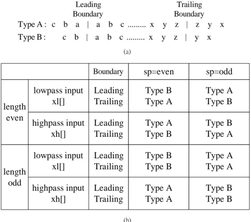
(5) α = − 1.586134342 , γ = 0.8829110762 , K 0 = 1.149604398 ,. β = −0.0529801185 4 , δ = 0.4435068522 , K 1 = 0.869864452 .. In forward transform, the computations are summarized as follows d i0 = x2i +1 , si0 = x2i , d i1 = d i0 + α × ( si0 + si0+1 ) , si1 = si0 + β × ( d i-11 + d i1 ) , d i2 = d i1 + γ × ( si1 + si1+1 ) , si2 = si1 + δ × ( d i-21 + d i2 ) , d i = K1 × d i2 , si = K 0 × si2 . Similarly, the inverse transform can be obtained by reversing the computations, that is si2 = K 0-1 × si , d i2 = K1−1 × d i , si1 = si2 − δ × ( d i-21 + d i2 ) , d i1 = d i2 − γ × ( si1 + si1+1 ) , si0 = si1 − β × ( d i-11 + d i1 ) , d i0 = d i1 − α × ( si0 + si0+1 ) , xˆ 2i = si0 , xˆ 2i +1 = d i0 In this paper, we adopt the separable approach to implement a 2-D DWT via the row-column operations of 1-D DWT. Note that a video object, after decomposition, may contain several line segments of different lengths in each 1-D line slice. To incorporate shape adaptive feature, the 1-D DWT should be able to 1) keep track of the starting point (SP) and the length of each line segment, and 2) perform length adaptive transform. The line segment information required in 1) can be obtained from the shape mask associated with a video object. A dedicated address generator is then employed to retrieve correct texture signals from a linear space memory as the 1-D SA-DWT input. One of the major challenges in DWT design is the boundary extension problem at both the leading and trailing edges of a line segment. This problem is further complicated under the shape adaptive scenario. There are two types of boundary extension. In type A extension, the end point inclusive and the neighboring pixels are mirrored to form the extension. In type B extension, the end point is excluded. In an odd symmetric convolution based SA-DWT, the type B boundary extension is always used at both leading and trailing boundaries in forward transform. As shown in Figure 2, The extension types used in inverse transform, however, depend on the filter type (high pass or low pass), the starting point position (even or odd) and the line segment length (even or odd). This leads to a very complicated design to handle the boundary extension. The boundary extension problem is somewhat alleviated in the lifting scheme. Table 1 shows the boundary extension scheme we derive for the lifting based SA-DWT and SA-IDWT. The padding zeros in the trailing edge are used to flush the data to the final stage.

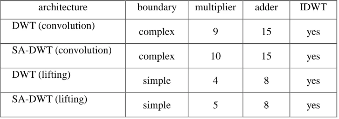
(6) and the padding length depends on the number of stages in the lifting scheme. The scheme exception occurs when the line segment length equals to 1. In forward transform, the single point data is multiplied by a constant of. 2. and treated as either low pass or high pass filter output. depending on the point position. In other words, if the position is odd, it will be classified as high pass filter output. In inverse transform, the single point data, coming from either low pass or high pass data streams, is divided by. 2. and stored by to the synthesis memory. Since the derived. scheme is very simple, the circuitry overhead is trivial and no speed penalty is paid. Table 2 summarizes the difference of design complexities for the four possible DWT schemes. When compared with the non-SA lifting based DWT, the incurred overhead of the proposed scheme is small, i.e. 1 additional multiplication. Leading Boundary Type A : c b a | a b c ......... x. Trailing Boundary y z | z y x. Type B :. y z | y x. c b | a b c ......... x (a). length even. length odd. Boundary. sp=even. sp=odd. lowpass input xl[]. Leading Trailing. Type B Type A. Type A Type B. highpass input xh[]. Leading Trailing. Type A Type B. Type B Type A. lowpass input xl[]. Leading Trailing. Type B Type B. Type A Type A. highpass input xh[]. Leading Trailing. Type A Type A. Type B Type B. (b). Figure 2. (a) boundary extension types. (b) the boundary extensions for the inverse transform of a convolution-based SA-DWT. Table 1. Boundary extension schemes for lifting based SA-DWT/SA-IDWT SP position. Leading edge. Trailing edge. even. Type B extension. Type B extension + padding zeros. odd. 1 padding zero + type B extension Type B extension + padding zeros.

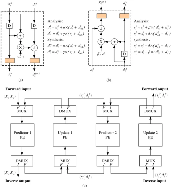
(7) Table 2. Compare of various VLSI architectures for Daubechies (9,7) filter. architecture DWT (convolution) SA-DWT (convolution) DWT (lifting) SA-DWT (lifting). boundary. multiplier. adder. IDWT. complex. 9. 15. yes. complex. 10. 15. yes. simple. 4. 8. yes. simple. 5. 8. yes. 3. ARCHITECTURE DESIGN OF 1-D LIFTING SA-DWT/IDWT In this paper, we follow the popular DWT design using Daubechies (9,7) filters. The design contains two lifting stages with each one containing a predict processor and an update processor. The block diagram designs of the predict processor, the update processor and the shared architecture design for both SA-DWT/IDWT are shown in Figure 3. Note that the splitting and the scaling stage designs are not shown for simplicity. The circuitry for the length one line segment is not shown, either. The add/sub operator performs addition in forward transform (analysis phase) and subtraction in inverse transform (synthesis phase). To reduce the critical path delay, pipelining registers are inserted to the outputs of both predict and update processors. For 2-D SA-DWT operation, a row-wise 1-D SA-DWT is performed first followed by a column-wise 1-D SA-DWT. Dedicated address generators are employed to access all the input data subject to the shape analysis. The starting point position and the line segment length information are calculated accordingly..

(8) sin. d in. D. D. .. S in+1. din. Analysis : 1 i. 1 i +1. ±. sin. 1 i. 0 i. 0 i +1. d = d − γ ×( s + s ) 1 i. α,γ. X. d = d − α ×( s + s ) 0 i. 2 i. 1 i. 1 i +1. +. 1 i. Synthesis : X. si1 = si0 + β × ( d i-11 + d i1 ). ±. d = d + γ ×( s + s ) 2 i. +. .. Analysis :. d i1 = d i0 + α × ( si0 + si0+1 ). β ,δ. D. .. sin. din+1 (a). .. si2 = s1i + δ × ( d i-21 + d i2 ) synthesis : si1 = si2 − δ × ( d i-21 + d i2 ) si0 = si1 − β × ( d i-11 + d i1 ). d in (b) Forward ouput. Forward input {si1, d i1}. {Xe, Xo}. {si2, di2}. F I MUX. I F DMUX. F I MUX. I F DMUX. Predictor 1 PE. Update 1 PE. Predictor 2 PE. Update 2 PE. DMUX I F. MUX F I. DMUX I F. MUX F I. {Xe, Xo} Inverse output. {si1, d i1}. {si2, di2} Inverse input. (c). Figure 3. (a) the predict processor, (b) the update processor (c) the lifting stage designs for forward and inverse SA-DWT 4. SA-ZTC SCHEME BASED ON MODIFIED SPIHT To preserve the coding efficiency obtained from SA-DWT, the zero tree coding scheme must be shape adaptive as well. Among various non-SA ZTC algorithm, SPHIT algorithm has been recognized as the one with highest compression efficiency. The SPHIT algorithm also supports progressive coding, which is a favorable feature for data transmission under limited channel bandwidth. Despite of its coding efficiency, the algorithm is far too complicated to be realized in hardware. It also needs to maintain a set of lists, e.g. LIS (list of insignificant set: for LL subband to record the zero tree roots that are not yet significant), LIP (list of insignificant pixels) and LSP (list of significant pixels). These require a large memory overhead to store the values. In this paper, we propose a new SA-ZTC scheme, which employs the same 4-coding-symbol set as that used in SPHIT but adopts a totally different coding algorithm. The algorithm features a.

(9) bottom-up and depth first scanning order in zero tree traversal. Figure 4 gives the details of the algorithm.. 1) Initialization: 1.1) set n = log 2 {max(c i, j )} as the number of texture bit-planes required in progressive coding. 1.2) for HL, LH, HH subbands, use DM(i,j) to identify if pixel (i,j) is within the decomposed shape mask. 1.3) for each subband in intermediate level k, use a size-4 buffer_k to record the significance information Sn(i,j) of wavelet coefficient cij. 1.4) for the top level, the refinement information SAQ(i,j) for the sequential approximation quantization is recorded in the buffer 2) Sorting Pass: 2.1) For the lowest pyramid level (k = 0): 2.1.1) for each wavelet coefficient cij, if DM(i,j) = 1, "1" significance output S n (i, j) =  "0" insignificance and store the values of Sn(i,j) into corresponding entries of buffer_k else store “10” into buffer_k 2.1.2) if Sn(i,j)=1 then output the sign of ci,j. and record SAQ(i,j)=1. 2.2) For the intermediate pyramid level (0 < k < N): 2.2.1) same as step 2.1.1; 2.2.2) same as step 2.1.2. "1" some descendents are siginificant 2.2.3) output SD(i, j ) =  "0" no descendent is significan 2.3) For the top pyramid level (k = N): 2.3.1) if DM(i,j)=1, output Sn(i,j), else skip to step 2.4; 2.3.2) same as step 2.2.2 2.3.3) same as step 2.2.3 2.4) For the root pyramid level (i.e. LL3), the coding is same as step 2.3. 3) Refinement Pass: for each SAQ(i,j)=1, output the nth most significant bit of |ci,j|;.

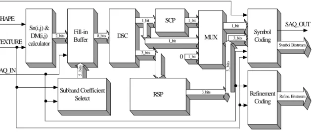
(10) 4) Quantization-Step Update: decrement n by 1 and go to Step 2. Figure 4. The proposed SA-ZTC algorithm 5. ARCHITECTURE DESIGN OF THE SA-ZTC ALGORITHM. Unlike SA-DWT, the SA-ZTC scheme requires separate encoder and decoder designs. Figure 5 shows the encoding processing element (EPE) design for each subband. SIGN. SHAPE. . . .. SAQ_IN. 1_bit. SAQ_OUT. 1_bit 2_bits. Fill-in Buffer. 8_bits. DSC. MUX. 1_bit. Symbol Coding. 3_bits. Symbol Bitstream 3_bits. 0. 1_bit 3_bits. .. SCP. 1_bit. 5_bits. Sn(i,j) & DM(i,j) TEXTURE calculator. Subband Coefficient Seletct. RSP. 3_bits. . .. Refinement Coding. Refine. Bitstream. Figure 5. The EPE block diagram of the SA-SPIHT. Concurrent processing of different subbands is possible by employing one EPE for each subband. The EPE first receives wavelet coefficients as well as the shape mask from the external memory. Note that the coefficients are decomposed into sign bit and magnitude (texture) parts. The “Sn(i,j) & DM(i,j) calculator” generates two-bit information Sn(i,j) and DM(i,j) subject to inputs. The values are also stored to the buffer_k in the “fill-in buffer” block to facilitate the descendent significance check performed by the upper level. For intermediate and top level processing, a one bit information SD(i,j) to indicate the significance of the descendents must be generated. This is accomplished in the “descendent significance check” (DSC) block. If all the descendent nodes of the current pixel turn out to be insignificant, the corresponding Sn(i,j) generated previously, however, must be removed from the output list. Since those descendent nodes with DM(i,j) = 0 are not coded at all, the number of Sn(i,j) to be removed varies from 0 to 4. This count is calculated in the “redundant symbol process” (RSP) block. Note that Sn(i,j) bits are not output directly. They are combined with the sign bit and the SD(i,j) to form the output symbol stream. This is performed in the “symbol coding” block. The output bit stream is pushed into a stack memory first. After all the wavelet coefficients in a pyramid are coded, it will be popped out.

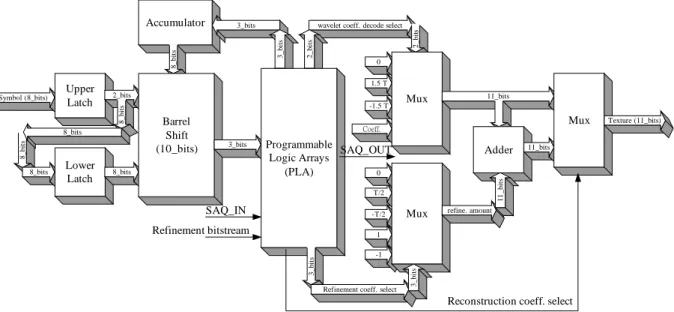
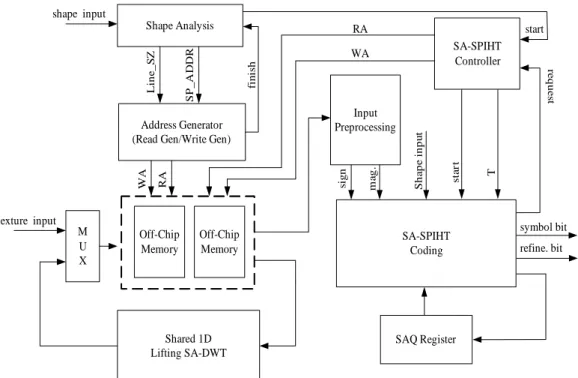
(11) for transmission. The “refinement coding” block is in charge of bit stream generation after the coding entering the refinement mode. Figure 6 shows the decoding processing element (DPE) for all subbands. Since the length of each receiving symbol varies, ranging from 1 to 3, a variable length decoding (VLD) process is needed to decode the symbol bit-stream. The VLD contains the two latches (as the decoding buffer), a 10-bit barrel shifter (BS), a 3-bit accumulator and a programmable logic array (PLA). The two latches form a 10-bit wide decoding buffer and the barrel shifter retrieves a 3-bit wide segment as the decoding frame. The barrel shifter acts like a 3-bit wide sliding window of the input data stream. The accumulator keeps track of the boundary of the last decoded symbol in the input latches and controls the displacement of the barrel shifter. The symbol decoding process is hardwired into an PLA, which generates both the value and the length of the decoded symbol. Additional inputs to the PLA are the SAQ_in signal and the refinement bit stream. Depending on whether the decoding is in the refinement mode, an appropriate symbol value is selected from the two multiplexers. The adder is employed for the refinement process.. 8_bits. Lower Latch. 2_bits. 2_bits. 1.5 T 2_bits. 8_bits. 8_bits. 0. -1.5 T. Barrel Shift (10_bits). Mux. 11_bits. Mux. Coeff. 3_bits. 8_bits. Programmable SAQ_OUT Logic Arrays (PLA) 0. Adder. T/2. SAQ_IN. -T/2. Refinement bitstream. Texture (11_bits). 11_bits. 11_bits. Upper Latch. 8_bits. Symbol (8_bits). wavelet coeff. decode select 3_bits. 3_bits. 8_bits. Accumulator. Mux. refine. amount. Refinement coeff. select. 3_bits. 3_bits. 1 -1. Reconstruction coeff. select. Figure 6. The DPE block diagram of the SA-SPIHT. Figure 7 illustrates the overall architecture design of a progressive image coding based on the lifting SA-DWT. It contains a 1-D lifting SA-DWT core, a shape analysis block, external memory address generators, a coding engine and a controller. The design also requires two single port off-chip memory modules working at twice the SA-DWT processing rate. We do not favor a two-port memory module in that the total pin count of the chip design will be increased dramatically. In addition, current memory technology does support a data rate up to 133MHz. For.

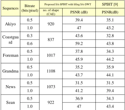
(12) the largest possible frame size, i.e. 1024×1024, each external memory module is of size 1M words. The flow begins with the shape analysis block which first receives shape mask information, performs shape decomposition and comes out with the length (Line_SZ) and the starting point address (SP_ADDR) of each line segment for the 1-D SA-DWT processing. The address generator, subject to the boundary extension scheme, generates appropriate read/write address to the external memory modules. Both the original image data and the computed wavelet coefficients are stored in external memory. The 1-D SA-DWT core processes the row-wise data first, and then the column-wise intermediate data next to accomplish the 2-D SA-DWT computations. This is followed by the SA-ZTC processing. The final adaptive arithmetic coding (AAC) block is not shown. shape input start SA-SPIHT Controller. finish. WA. texture input M U X. Off-Chip Memory. Off-Chip Memory. Shared 1D Lifting SA-DWT. SA-SPIHT Coding. T. start. Shape input. RA. mag.. Input Preprocessing. sign. Address Generator (Read Gen/Write Gen) WA. RA. request. Line_SZ. SP_ADDR. Shape Analysis. symbol bit refine. bit. SAQ Register. Figure 7. The overall architecture of the proposed progressive image coding system 6. EXPERIMENTAL RESULTS AND PERFORMANCE CCOMPARISONS. To demonstrate the coding efficiency of the proposed lifting SA-DWT and SA-SPIHT scheme, we conducted several performance experiments using several QCIF format sequences in monochrome 8-bit pixel format. The DWT filter is of type Daubechies (9,7) and a 3-level decomposition is performed. The comparison is against the non-SA SPHIT algorithm and the results are compiled into Table 3. Note that the SA version SPHIT is not available so far and the data bits for the shape mask information are counted in this comparison. In most benchmarks (except for the grandma case), the proposed scheme has a significant performance edge over the SPHIT algorithm. For a fixed bit rate coding, the PSNR difference can be as large as 15dB. In.

(13) average, the gain is about 4dB. Figure 8 shows the Sean and Akiyo cases under different bit rate. The curves clearly exhibit a 4dB gap between the two schemes. Figure 9 shows the decoded illustration of Sean-QCIF image under 0.5b/pixel and 1b/pixel bit rates. Table 3 the performance compare our proposed approach and SPIHT. Sequences. Bitrate (bits/pixel). Akiyo Coastgua rd Foreman. 0.5 1.0 0.3 0.6 0.5. Proposed SA-SPIHT with lifing SA-DWT. no. of shape (CAE). 920. 837. 1017. 1.0 Grandma. News. Sean. (a) Sean-QCIF. 0.5 1.0 0.5 1.0 0.5 1.0. 1108. 1073. 922. SPIHT [9]. PSNR (dB). PSNR(dB). 39.4. 35.1. 47. 43.2. 43.6. 32.8. 59.2. 43.8. 37.8. 34.3. 45.9. 44.2. 35.2. 35.9. 43.7. 44.1. 31.5. 31.5. 41.2. 39.4. 36.9. 34.3. 47. 43.4. (b) Akiyo-QCIF. Fig. 8 Performance comparison between the proposed schemes, SPHIT..

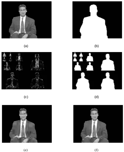
(14) (a). (b). (c). (d). (e). (f). Figure 9. Original and decoded Sean-QCIF (a) Original image. (b) Original Shape mask. (c) Three-level decomposition by lifting SA-DWT. (d) Three-level decomposition of the shape mask. (e) decoded result for bitrate=0.5 b/pixel (f) decoded result for bitrate=1.0 b/pixel 7. VLSI IMPLEMENTATION RESULTS AND DESIGN SUMMARY. To verify the hardwired performance, the proposed design is realized in VLSI using TSMC 0.35um 1P4M process. Since SA-DWT is the more computation intensive module and the memory access schemes between the SA-DWT and SA-ZTC need further investigation for minimum communication overhead, only SA-DWT is incorporated into the design. The implementation results are shown in Table 4. The core size is around 1800 ×1800 um2 and the gate count is around 18,600. To reduce the critical path delay formed by the MAC path in the predict and the update processors, a 10-bit CSD data format is employed in multiplication scheme. This cuts the critical path delay to about 16.6ns and an approximately 60MHz clock rate can be achieved. The computing power implies a sustained processing rate of 42 frames/sec for size 1024×1024 images..

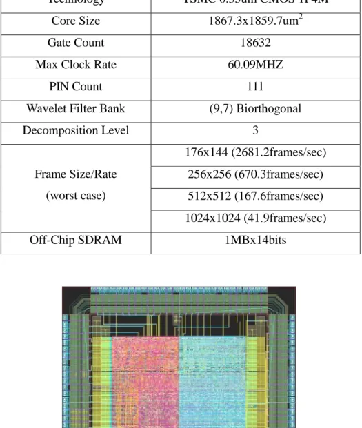
(15) Table 4. VLSI implementation results of SA-DWT Technology. TSMC 0.35um CMOS 1P4M. Core Size. 1867.3x1859.7um2. Gate Count. 18632. Max Clock Rate. 60.09MHZ. PIN Count. 111. Wavelet Filter Bank. (9,7) Biorthogonal. Decomposition Level. 3 176x144 (2681.2frames/sec). Frame Size/Rate. 256x256 (670.3frames/sec). (worst case). 512x512 (167.6frames/sec) 1024x1024 (41.9frames/sec). Off-Chip SDRAM. 1MBx14bits. Figure 10. Chip layout view of the SA-DWT design In conclusion, this paper presents an efficient algorithm and its VLSI architecture design for forward and inverse lifting SA-DWT. We have successfully incorporated the SA feature into the lifting DWT scheme and resolve the boundary extension problem with minimum overheads. In addition, a high performance SA-ZTC scheme based on modified SA-SPIHT algorithm is also presented. Experimental results show that the proposed scheme can achieve better coding.

(16) efficiency than the original SPHIT algorithm. The proposed architecture design is also the first one reported capable of realizing such complicated ZTC algorithm in hardware. REFERENCES. [1] Chu Yu; Sao-Jie Chen, “Design of an efficient VLSI architecture for 2-D discrete wavelet transforms, ” IEEE Consumer Electronics, Volume: 45 Issue: 1, Feb. 1999 Page(s): 135 -140. [2] Jer Min Jou; Yeu-Horng Shiau; Chin-Chi Liu, “Efficient VLSI architectures for the biorthogonal wavelet transform by filter bank and lifting scheme, ” IEEE Circuits and Systems. ISCAS 2001, Volume: 2 , 2001 Page(s): 529 -532 vol. 2 [3] Chung-Jr Lian; Kuan-Fu Chen; Hong-Hui Chen; Liang-Gee Chen, “Lifting based discrete wavelet transform architecture for JPEG2000, “IEEE Circuits and Systems. ISCAS 2001, Volume: 2 , 2001 Page(s): 445 -448 vol. 2 [4] W. Sweldens, “The lifting scheme: A custom design construction of biorthogonal wavelets,” Applied Comput. Harmon. Analysis, pp. 186-200, 1996 [5] Shipeng Li; Weiping Li, “Shape-adaptive discrete wavelet transforms for arbitrarily shaped visual object coding,” IEEE Circuits and Systems for Video Technology, Volume: 10 5, Aug. 2000, Page(s): 725 –743 [6] C.-T. Huang, P.-C. Tseng and L.-G. Chen, “VLSI implementation of shape-adaptive discrete wavelet transform,” 12th VLSI/CAD Symp., C1-1, Hsinchu, Taiwan, Aug. 2001 [7] Shapiro, J.M., “Embedded image coding using zerotrees of wavelet coefficients,” IEEE Signal Processing, Volume: 41 12, Dec. 1993, Page(s): 3445 –3462 [8] Said, A.; Pearlman, W.A., “A new, fast, and efficient image codec based on set partitioning in hierarchical trees,” IEEE Circuits and Systems for Video Technology, Volume: 6 3, June 1996, Page(s): 243 –25 [9] Shen-Fu Hsiao; Yor-Chin Tai; Kai-Hsiang Chang, “VLSI Design of an efficient embedded zerotree wavelet coder with function of digital watermarking,“ IEEE Consumer Electr.,. Volume: 46 3 , Aug. 2000 , Page(s): 628 –636.

(17)