最大輸入編碼色彩重現之四原色色域最佳化設計

全文

(1)國立交通大學顯示科技研究所碩士論文最大輸入編碼色彩重現之四原色色域最佳化設計 Optimum Design of Four-primary Color Gamut for Reproducing Maximum Input Encoded Color. 研究生：陳勇智. 指導教授：謝漢萍教授. 中華民國九十六年六月.

(2) 最大輸入編碼色彩重現之四原色色域最佳化設計 Optimum design of Four-primary Color Gamut for Reproducing Maximum Input Encoded Color. 研究生：陳勇智指導教授：謝漢萍. Student : Yong-Jhih Chen Advisor : Han-Ping D. Shieh. 國立交通大學電機學院顯示科技研究所碩士論文 A Thesis Submitted to Display Institute College of Electrical Engineering and Computer Science National Chiao Tung University in Partial Fulfillment of the Requirements for the Degree of Master in Display Institute June 2007 Hsinchu, Taiwan, Republic of China 中華民國九十六年六月.

(3) 最大輸入編碼色彩重現之四原色色域最佳化設計碩士研究生：陳勇智. 指導教授：謝漢萍教授. 國立交通大學. 顯示科技研究所. 摘. 要. 為擴大顯示器色域以呈現更生動且自然的色彩，近年來已吸引許多顯示器專家及廠商投入多原色技術的發展。相較於傳統顯示器之設計，多原色顯示器保有色域設計的彈性。然而，惟有透過適切的色域轉換之影像編碼，消費者才有機會享受大色域顯示器所呈現的豐富鮮豔色彩。本論文提出重現最大輸入編碼色彩之(四原色)色域最佳化設計的方法。基於最大色域體積重疊的條件，此方法可達到高傳真的色彩重現目的。為實際比較並驗證基於不同演算法所獲得之最佳化色域，本研究設計一組背光模組（暨驅動電路）作為驗證平台，並採用四原色發光二極體為光源，令該背光模組具備呈現不同色域之彈性。本研究以兩種主要編碼色域－“標準 RGB”及“真實表面色域”作為輸入色域，分別依循兩種常用演算法則－最大白點亮度與最大設計色域體積要求，以及本論文所建議之最大輸入色域體積重疊要求進行計算，並依據所得結果進行交差比對。結果顯示使用本方法可重現最大輸入色域。此外，若應用於最新發展的大色域輸入編碼訊號，將可以使多原色顯示器顯示出更接近人眼視覺系統的色域表現範圍。. i.

(4) Optimum Design of Four-primary Color Gamut for Reproducing Maximum Input Encoded Color Student: Yong-Jhih Chen. Advisor: Dr. Han-Ping D. Shieh. Display Institute National Chiao Tung University. Abstract In order to widen the display color gamut for providing more vivid and natural color perception, many of researchers and manufacturers were attracted to invest in the development of multi-primary technology in recent years. Comparing to the conventional displays, multi-primary displays (MPDs) offer the flexibility to adjust and exhibit possible color gamut volume (CGV). However, only through proper encoding gamut conversion, consumers could have the chance to enjoy the vivid color image on the large gamut display. This thesis presents a method to design the optimal (four-primary) color gamut for reproducing maximum number of input encoded color. Based on the maximum color gamut volume intersection requirement, the high-fidelity color reproduction can be achieved. For actually comparing and evaluating the optimum color gamut based on different algorithms, a backlight module (and the driving circuit) was constructed as a platform for verification. A set of four four-primary LEDs were adopted as the light sources, which offer the flexibility to have the different color gamut on the backlight module. Two major encoding color gamuts, “sRGB” and “real surface color gamut,” are chosen as input gamuts. Calculations are performed under two commonly-adopted criteria, maximum white point luminance and maximum designed CGV, and the proposed one, maximum intersectional CGV, respectively. Result shows the proposed method, compared to others, is demonstrated to reproduce maximum input color gamut. Moreover, if applying the method to the new developed large color gamut input encoding signal, the MPDs will display the color gamut toward the gamut range of human visual system. ii.

(5) 誌. 謝. 首先誠摯的感謝指導老師謝漢萍教授，在這碩士兩年中對於研究態度及英文能力的教導，以及提供豐富的資源與完善研究環境，使我得以在碩士生涯提升了專業及英文的能力，順利完成此論文。此外，也感謝各位口試委員所提供的寶貴意見，使本論文更加的完備。. 在此特別感謝鄭裕國學長對於論文的指導，細心的指導方式，嚴謹的研究態度，讓我更能學習成長，受益良多。另外，本論文的完成亦得感謝點晶科技吳華冑先生對於實驗元件的提供，促使實驗平台的完成。. 在實驗室的日子裡，感謝有鄭榮安、林芳正、楊柏儒、方仁宇、陳均合、莊喬舜、李企桓等經驗老到、學識豐富的學長姐們提供各方面的指導與協助，同時感謝侑興、坤岳、友群、振宇、韻竹、雅婷等同學們在課業、研究、生活上的幫助與分享，並伴我一起度過兩年碩士班的日子。我也感謝實驗室的學弟妹們與助理小姐，感謝你/妳們的幫忙及讓實驗室充滿歡愉的氣氛。與實驗室成員們歡樂辛酸的毎一天，我將銘感在心。. 最後，我要呈上我最多的歉意和謝意給予我心愛的女友－貽姍及我最敬愛的家人，他們的體諒和關愛是支持我一路走來最大的支柱，使我能無後顧之憂的研究與學習，並順利完成碩士學業。如今我即將邁入人生的另一個階段，在未來的日子裡我必當竭盡所能來回報你們。在此，我將這份喜悅與每位關心我的人分享。. iii.

(6) Table of Contents Abstract (Chinese)…………………………………………………………………..i Abstract (English)…………………………………………………………………..ii Acknowledgment…………………………………………………………………..iii Table of Contents …………………………………………………………………..iv Figure Captions ………….…………………………………………………………vi List of Tables …………….…….………………………………………………….ix. Chapter 1. Introduction ................................................................................... 1. 1.1 Color gamut of multi-primary display.............................................................................1 1.1.1 Different color gamut ...............................................................................................1 1.1.2 Widening color gamut ..............................................................................................3 1.1.3 Multi-color-LED backlight in field sequential .........................................................4 1.2 Color reproduction...........................................................................................................7 1.2.1 Gamut mapping ........................................................................................................8 1.2.2 Color conversion issues............................................................................................9 1.3 Motivation and objective of this thesis.......................................................................... 11 1.4 Organization of this thesis .............................................................................................12. Chapter 2. Principle of Color Gamut Design .............................................. 13. 2.1 Colorimetry....................................................................................................................13 2.1.1 CIEXYZ color space ..............................................................................................14 2.1.2 CIELUV color space ..............................................................................................15 2.1.3 CIELAB color space...............................................................................................17 2.2 Previous work - Wen’s method......................................................................................18 2.3 Proposed method ...........................................................................................................23 2.4 Test input color gamuts..................................................................................................27 2.4.1 Standard RGB color space (sRGB) ........................................................................27 2.4.2 Real-world surface colors gamut............................................................................29. Chapter 3. Experiment and Simulation ....................................................... 31. 3.1 Experiment.....................................................................................................................31 iv.

(7) 3.1.1 Four-primary-LED backlight platform...................................................................31 3.1.2 Measurement equipment ........................................................................................34 3.1.3 Measurement data...................................................................................................36 3.2 Simulation......................................................................................................................39 3.2.1 Numerical analysis .................................................................................................39 3.2.2 Gamut visualization................................................................................................39 3.2.3 Q-hull algorithm .....................................................................................................40. Chapter 4. Results & Discussion................................................................... 41. 4.1 sRGB color gamut as the input......................................................................................41 4.1.1 Maximum white point luminance...........................................................................41 4.1.2 Maximum four-primary CGV ................................................................................43 4.1.3 Maximum input CGV intersection .........................................................................44 4.1.4 Summary.................................................................................................................46 4.2 Real surface color gamut as the input............................................................................49 4.2.1 Maximum white point luminance...........................................................................49 4.2.2 Maximum four-primary CGV ................................................................................51 4.2.3 Maximum input CGV intersection .........................................................................52 4.2.4 Summary.................................................................................................................54 4.3 Discussion......................................................................................................................57. Chapter 5. Conclusions & Future Work ...................................................... 59. 5.1 Conclusions ...................................................................................................................59 5.2 Future work....................................................................................................................61. Reference............................................................................................................. 62 Appendix ............................................................................................................. 64. v.

(8) Figure Captions Fig. 1-1. The CIE xy chromaticity diagram with the color gamuts of NTSC and a..................2 Fig. 1-2. The displays with different NTSC ratio color gamut..................................................3 Fig. 1-3. Timing of the driving scheme of four color LEDs for modulating color gamut.........5 Fig. 1-4. Illustration of color gamut modulation of four color LEDs........................................5 Fig. 1-5. The white point decided by the relative luminance of four-primary LEDs: (a) a high color temperature setting, (b) a low color temperature setting..................................................6 Fig. 1-6. Basic color reproduction process through device-independent color space ...............7 Fig. 1-7. The gamut transformation of color reproduction process...........................................8 Fig. 1-8. The illustration of gamut mapping..............................................................................9 Fig. 2-1. The matching functions fitted to the spectral responses of human eye ....................15 Fig. 2-2. The volume of visible colors in the CIEXYZ color space, the triangle is on the X + Y + Z = 1 plane............................................................................................................................15 Fig. 2-3. The 1976 u’v’ chromaticity diagram and its color difference diagram.....................16 Fig. 2-4. Luminance Yr, Yg, and Yb plotted against Yy under the white point requirement (S. Wen, Displays, 26, pp. 171-176, 2005) ...................................................................................21 Fig. 2-5. Luminance ratios Yrm/Yr, Ygm/Yg, Ybm/Yb, and Yym/Yy plotted against Yy (S. Wen, Displays, 26, pp. 171-176, 2005) ............................................................................................22 Fig. 2-6. The CGV (ΔΕ*ab3) of four-primary display plotted against Yy (S. Wen, Displays, 26, pp. 171-176, 2005) ..................................................................................................................23 Fig. 2-7. The design flow of proposed method........................................................................26 Fig. 2-8 The Pointer color gamut in CIE xy chromaticity diagram ......................................30 Fig. 3-1. The photo of four-primary-LED backlight platform, which included (a) a optical cavity, (b) a constant-current driving board, and (c) FPGA control signal board ...................32 Fig. 3-2. The photo of simple optical cavity and the correlative specification of LED ..........32 Fig. 3-3. The photo of constant-current driving board and its description..............................33 Fig. 3-4. The photo of Conoscope ...........................................................................................34 vi.

(9) Fig. 3-5. The luminous information path in Conoscope..........................................................35 Fig. 3-6. The principle diagram of Conoscope........................................................................36 Fig. 3-7. Four-primary color gamut compared with standard color space in CIE 1976 UCS diagram ....................................................................................................................................37 Fig. 3-8. Luminance of each primary plotted against digital count of control circuit.............37 Fig. 3-9. The plot of different digital count (dived in to 8 level) in the CIE xy chromaticity diagram ....................................................................................................................................38 Fig. 3-10. The concept of convex hull in gamut visualization ................................................40 Fig. 3-11. The simple illustration of q-hull algorithm method ................................................40 Fig. 4-1. Plots of luminances Yr, Yg, and Yb as functions of Yc under the white point requirement..............................................................................................................................42 Fig. 4-2. Plots of luminance ratios Yrm/Yr, Ygm/Yg, Ybm/Yb, and Ycm/Yc as functions of Yc under the white point requirement.....................................................................................................43 Fig. 4-3. The available LED efficiency plotted against Yc under the sRGB gamut input.......43 Fig. 4-4. The four-primary CGV plotted against Yc under the sRGB gamut input .................44 Fig. 4-5. Plot of intersectional CGV as a function of the shifted Yc value under sRGB gamut input .........................................................................................................................................45 Fig. 4-6. 3D visualization of four-primary gamut in CIELAB color space with different angle of (a) top and (b) side view ..........................................................................................................45 Fig. 4-7. 3D visualization of sRGB color gamut in CIELAB color space with different angle of (a) top and (b) side view ..........................................................................................................46 Fig. 4-8. 3D CGV Intersection of four-primary gamut and sRGB gamut...............................46 Fig. 4-9. Efficiency, four-primary CGV, and the intersectional CGV plotted against Yc for comparison with sRGB gamut input .......................................................................................47 Fig. 4-10. Plots of luminances Yr, Yg, and Yb as functions of Yc under the white point requirement..............................................................................................................................50 Fig. 4-11. Plots of luminance ratios Yrm/Yr, Ygm/Yg, Ybm/Yb, and Ycm/Yc as functions of Yc under the white point requirement...........................................................................................51 Fig. 4-12. The available LED efficiency plotted against Yc under real surface gamut input ..51 vii.

(10) Fig. 4-13. The four-primary CGV plotted against Yc under the real surface gamut input ......52 Fig. 4-14. Plot of intersectional CGV as a function of the shifted Yc value under real surface gamut input ..............................................................................................................................53 Fig. 4-15. 3D visualization of four-primary gamut in CIELAB color space with different angle of (a) top and (b) side view......................................................................................................53 Fig. 4-16. 3D visualization of real surface color gamut in CIELAB color space with different angle of (a) top and (b) side view ............................................................................................54 Fig. 4-17. 3D CGV Intersection of four-primary gamut and real surface color gamut ...........54 Fig. 4-18. Efficiency, four-primary CGV, and the intersectional CGV plotted against Yc for comparison with real surface gamut input...............................................................................55 Fig. 5-1. The algorithm of two type gamut mappings of the large gamut display ..................61. viii.

(11) List of Tables Table 2-1 Parameters of sRGB chromaticties..........................................................................28 Table 2-2 Parameters of sRGB viewing environment .............................................................29 Table 3-1 LED specifications and measurement data .............................................................36 Table 4-1 The relative luminance setting of each criterion with sRGB gamut input ..............47 Table 4-2 The compared result of each criterion .....................................................................48 Table 4-3 The color difference with the reference white D65 in CIE 1976 UCS diagram of each criterion....................................................................................................................................48 Table 4-4 The relative luminance setting of each criterion with real surface gamut input .....54 Table 4-5 The compared result of each criterion .....................................................................56 Table 4-6 The color difference with the reference white C in CIE 1976 UCS diagram of each criterion....................................................................................................................................56 Table 4-7 The simplified comparison of each criterion...........................................................57. ix.

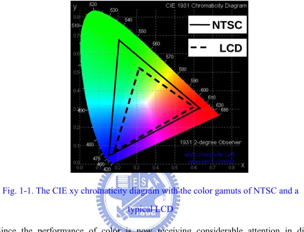
(12) Chapter 1. Introduction Color gamut [1], the range of color which can be reproduced by a device, is one of the general index to judge the color performance of a display. For widening the color gamut, several multi-primary displays (MPDs) [2], [3] were proposed to achieve vivid and natural color perception. However, the additional primaries will bring the color conversion issue due to the offered flexibility in color reproduction process [4]. In this chapter, the key issues of color gamut design in MPDs and the objective of this thesis will be discussed.. 1.1 Color gamut of multi-primary display 1.1.1 Different color gamut Color gamut of a device or a system is often quantified by comparison with National Television System Committee (NTSC) [5] standard in some engineering applications. The NTSC is the analog color television (TV) standard in the United States and defines the color and video information. The percentage of NTSC in the chromatic diagram is the reference index, which implies the approximate ratio of total color that can be theoretically displayed in a color TV system. As shown in Fig. 1-1, the color gamut is presented in the CIE 1931 xy chromaticity diagram. The horseshoe-shaped border represents the visual spectrum boundary of human eye. The gamut of NTSC and a typical liquid crystal display (LCD) [6] are represented by the solid- and dashed- line triangles, respectively. As shown in the diagram, the color gamut of typical LCD is only 70% of NTSC and also far less than the gamut that human. 1.

(13) eye can see. Actually, the color gamut showed and compared in 2D chromaticity diagram just for convenience. The “real color gamut” is operated and visualized in the three dimensional color spaces, which will be described in next chapter.. NTSC LCD. Fig. 1-1. The CIE xy chromaticity diagram with the color gamuts of NTSC and a typical LCD Since the performance of color is now receiving considerable attention in display technology, larger color gamut display for presenting more color and higher color saturation image is increasing demand from display manufacturers. The performances of two commercial LCDs with different color gamut are shown in Fig. 1-2. The right LCD, which has 90% of NTSC is much larger than the left one, which only has 72% of NTSC. Obviously, the right one which has the larger gamut performs the more vivid and natural color perception than the left one.. 2.

(14) 72% NTSC. 90% NTSC. Fig. 1-2. The displays with different NTSC ratio color gamut. 1.1.2 Widening of color gamut Currently, there are two major methods proposed for widening the color gamut of displays. The first use the saturated primaries [7], and the second use the multi-primaries [8]. For example, the color gamut of recent most important information display device, LCD, is determined by the combination of the spectral characteristics of backlight source and the spectral transmission factors of color filters. Since the conventional light source, cold cathode fluorescent lamp (CCFL), has the wider band spectrum, some lights leak to the not intended wavelength of color filters result in a poor color separation. For providing the saturated primaries with narrow spectrum, some researchers replaced CCFL with the light-emitting diode (LED) [7], thus making it easier to separate colors by the color filters. Besides the above mentioned proposal, the most efficient way to enlarge the color gamut of display significantly was to increase the number of primaries. Therefore, some researches proposed and demonstrated the MPDs either of the sequential or spatial type to increase the color gamut [9], [10].. 3.

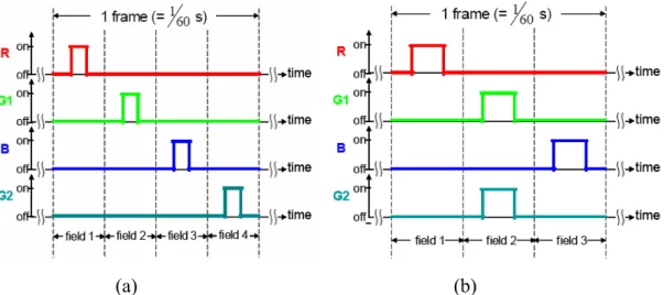
(15) 1.1.3 Multi-color-LED backlight in field sequential As previously noted, multi-primary display (MPD) is the proper method to widen the color gamut. A four-primary-LED backlight in the field-sequential full-color (FS-FC) LCDs [11] was proposed, due to its high luminous efficiency and large color gamut. Furthermore, the extra advantages to modulate the color gamut and color temperature efficiently were brought simultaneously. Thus, this thesis based on this structure examines the proposed method in the following chapter. Modulation of the color gamut Since the FS-FC LCD replaces the color filters with the color sequential LED backlight, the effective primaries or color gamut are decided by the sequential LED signals and transmitted characteristic of the liquid crystal. For example, the timing of driving scheme of the four color LEDs is schematically represented in Fig. 1-3. As shown in Fig. 1-3(a), when sequentially turn on the four LED backlights R,G1,B,and G2, the quadrangle color gamut will much larger than the NTSC color gamut in the chromaticity diagram, as shown in Fig. 1-4. Moreover, if G1 and G2 are operated simultaneously, as shown in Fig. 1-3(b), the coordinate of G’ (refer to Fig. 1-4)is the result from the combination of G1 and G2 by properly tuning the relative luminance. Then, the effective dynamic three primary color gamut RG’B can be adjusted by preference design.. 4.

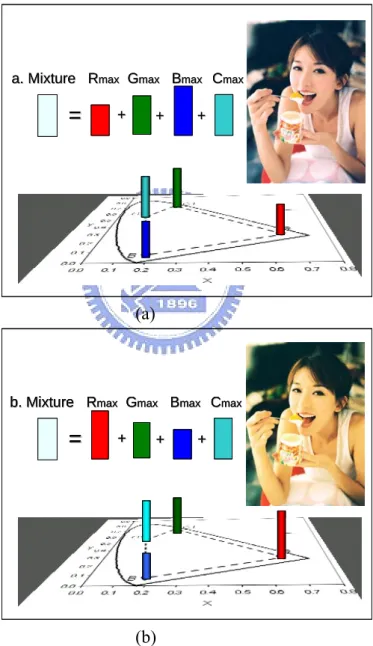
(16) (a). (b). Fig. 1-3. Timing of the driving scheme of four color LEDs for modulating color gamut : (a) Sequential turn on RG1BG2 LEDs, (b) G1 and G2 are operated in the same field. CIE 1931 xy coordinate 0.9. 100% NTSC. 0.8. G1. G’. 0.7. 4-Primary User set. G2. 0.6. 3-primary. 0.5. y. 0.4. R. 0.3 0.2 0.1. B. 0.0 0.0. 0.1. 0.2. 0.3. 0.4. 0.5. 0.6. 0.7. 0.8. x. Fig. 1-4. Illustration of color gamut modulation of four color LEDs Modulation of the color temperature Color temperature that dominantly affects the color performance is the characteristic of the white point of a display, and the white point is decided by the relative luminance of each primary. Due to the very nature of field sequential method and the current-controlled LEDs, the desired color temperature can be obtained by applying well-calculated timing and driving 5.

(17) current to each LED of the backlight system. After the calculation, operating currents of each LED are acquired to drive the LEDs to achieve the target color temperature. As shown in Fig. 1-5, Fig. 1-5(a) is the high color temperature setting and Fig. 1-5(b) is the low color temperature setting, each having different relative ratio of primaries that performs different perceptions. Since the LEDs are separately controlled, it is easy to modulate the color temperature of LCDs by tuning the proportionality of luminance between the primary colors.. a. Mixture Rmax Gmax Bmax Cmax. =. +. +. +. (a). b. Mixture Rmax Gmax Bmax Cmax. =. +. +. +. (b) Fig. 1-5. The white point decided by the relative luminance of four-primary LEDs: (a) a high color temperature setting, (b) a low color temperature setting. 6.

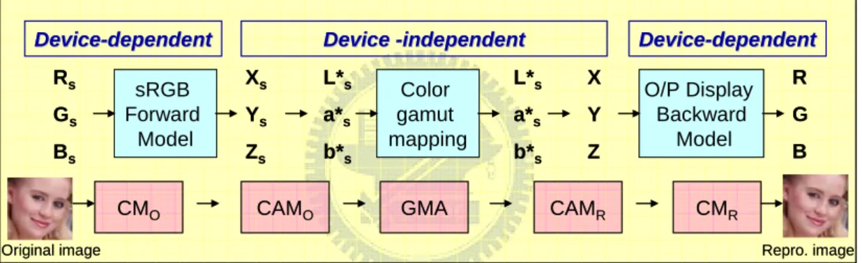
(18) 1.2 Color reproduction Many types of electronic imaging devices, including color cathode ray tube (CRT) devices, ink jet printers, LCDs, etc. utilize the device-dependent color spaces for color specification. However, device-dependent color spaces do not relate to an objective definition of color or human color perception. Therefore, the device-independent color spaces [12] developed by International Commission on Illumination (CIE) give a quantitative measure for all colors that is not dependent on the imaging device. As a result, the production of color consistency between various devices, i.e., the concept of device-independent color reproduction, as shown in Fig. 1-6, has been received widespread attention.. DeviceDevice-dependent Rs Gs Bs. sRGB Forward Model CMO. Device -independent Xs. L*s. Ys. a*s. Zs. b*s. CAMO. Color gamut mapping GMA. DeviceDevice-dependent. L*s. X. a*s. Y. b*s. Z CAMR. Original image. O/P Display Backward Model. R G B. CMR Repro. image. Fig. 1-6. Basic color reproduction process through device-independent color space The six types of color reproduction were defined by Hunt [13] as follows: spectral color reproduction, colorimetric color reproduction, exact color reproduction, equivalent color reproduction, corresponding color reproduction, and preferred color reproduction. Each of these types of color reproduction is separated according to purpose. Nowadays, the research related to reproducing images on MPD was classified into two main areas. The first one was based on multi-spectral information [14], such as the spectral reflectance of an object estimated by a multi-spectral camera or some measured spectrum data. This type of reproduction tends to reproduce the original color, i.e., natural color reproduction, which can reproduce more realistic image, but can not be directly applied to current High-definition. 7.

(19) television (HDTV) system. The other one was based on the colorimetric information [15], such as standard RGB (sRGB) and CIEXYZ, for applying the current color management system. This type of reproduction also can reproduce the original color and tend to reproduce the preference color, i.e., preference color reproduction [16], which can produce the memory color of people preferred but need some psychophysical experiment to be evaluated. In this thesis, the measured colorimetric data was applied for the original color reproduction.. 1.2.1 Gamut mapping The color reproduction from the input color gamut to multi-primary color gamut needs a transformation, called gamut mapping, as shown in Fig. 1-7. The gamut mapping is a technique to transform out-of-gamut colors into within-gamut, and thereby solve the gamut-mismatch problem. Since the destination gamut of MPD is larger than the recent input color gamut, the mapping can be the original color mapping or preference color mapping. Furthermore, the gamut mapping is implemented in the device-independent color space, which is represented in three dimensions (3D), as shown in Fig. 1-8. Over the years, some strategies [17] has been using to solve the variant gamut mapping problem.. Input signal Color Gamut. Transformation processing. Destination Multi-primary Color Gamut. Fig. 1-7. The gamut transformation of color reproduction process. 8.

(20) Gamut1 Gamut2. Fig. 1-8. The illustration of gamut mapping. 1.2.2 Color conversion issues As previously noted, the device-independent color space provided by CIE is utilized for the color reproduction, and the device-independent color reproduction requires a color conversion between device color and device-independent color to achieve color consistency. Any color in a three primary system can only be expressed as a single combination of coordinates. For example, the relative primary luminances of a conventional three-primary display are uniquely determined by its white point. Refer to Fig. 1-6, in that case, the linearity and additivity of colorimetric characteristics of a display system are ensured; the forward model is shown as follows:. ⎡ X w ⎤ ⎡ X R _ max ⎢ ⎥ ⎢ ⎢ Yw ⎥ = ⎢ YR _ max ⎢⎣ Z w ⎥⎦ ⎢⎣ Z R _ max. X G _ max YG _ max Z G _ max. X B _ max ⎤ ⎡ R ⎤ ⎥ YB _ max ⎥ ⎢⎢G ⎥⎥ , Z B _ max ⎥⎦ ⎢⎣ B ⎥⎦. ⎡ R ⎤ ⎡TRC (d R ) ⎤ ⎢G ⎥ = ⎢TRC (d ) ⎥ G ⎥ ⎢ ⎥ ⎢ ⎢⎣ B ⎥⎦ ⎢⎣TRC (d B ) ⎥⎦. (1- 1). where R/G/B are the three primaries, Xi/Yi/Zi are the CIE XYZ tristimulus, di is the display signal, and TRC is a tone reproduction curve. Note: [i can be the three primaries (R, G, and B) and the white point (w)]. Then, a backward model defined as the inversion of a forward mode, is shown as follows:. 9.

(21) ⎡ R ⎤ ⎡ X R _ max ⎢G ⎥ = ⎢ Y ⎢ ⎥ ⎢ R _ max ⎢⎣ B ⎥⎦ ⎢⎣ Z R _ max. X G _ max YG _ max ZG _ max. X B _ max ⎤ ⎥ YB _ max ⎥ Z B _ max ⎥⎦. −1. ⎡Xw⎤ ⎢ ⎥ ⎢ Yw ⎥ , ⎢⎣ Z w ⎥⎦. −1 ⎡ d R ⎤ ⎡TRC ( R ) ⎤ ⎢ d ⎥ = ⎢TRC −1 (G ) ⎥ ⎥ ⎢ G⎥ ⎢ −1 ⎢ ⎢⎣ d B ⎥⎦ ⎣TRC ( B ) ⎥⎦. (1- 2). regarding the color management system, to solve the three linear equations in three unknowns, the signal di can be calculated by the white point of display. When the color conversion method applies on the MPD, such as the four-primary backlight, the forward model can be shown as follows:. ⎡ X ⎤ ⎡ X R _ max ⎢Y ⎥ = ⎢ Y ⎢ ⎥ ⎢ R _ max ⎢⎣ Z ⎥⎦ ⎢⎣ Z R _ max. X G _ max YG _ max Z G _ max. ⎡R⎤ X B _ max X C _ max ⎤ ⎢ ⎥ ⎥ G YB _ max YC _ max ⎥ ⎢ ⎥ , ⎢B⎥ Z B _ max Z C _ max ⎥⎦ ⎢ ⎥ ⎣C ⎦. ⎡ R ⎤ ⎡TRC (d R ) ⎤ ⎢G ⎥ ⎢TRC (d ) ⎥ G ⎥ ⎢ ⎥=⎢ ⎢ B ⎥ ⎢TRC (d B ) ⎥ ⎥ ⎢ ⎥ ⎢ ⎣ C ⎦ ⎣TRC (d C ) ⎦. (1- 3). where C, cyan, is the additive primary of the backlight system. In this model, the white point can be achieved by the setting of four-primary signals. However, the backward model of four-primary is shown as follows:. ⎡R⎤ ⎢G ⎥ ⎡ X R _ max ⎢ ⎥ = ⎢ YR _ max ⎢B⎥ ⎢ ⎢ ⎥ ⎢⎣ Z R _ max ⎣C ⎦. X G _ max. X B _ max. YG _ max Z G _ max. YB _ max Z B _ max. ⎡ d R ⎤ ⎡TRC −1 ( R ) ⎤ X C _ max ⎤ ⎡ X ⎤ ⎢ ⎥ ⎢ ⎥ −1 ⎥ ⎢ ⎥ ⎢ dG ⎥ ⎢TRC (G ) ⎥ YC _ max ⎥ ⎢ Y ⎥ , (1- 4) = ⎢ d B ⎥ ⎢TRC −1 ( B ) ⎥ Z C _ max ⎥⎦ ⎢⎣ Z ⎦⎥ ⎢ ⎥ ⎢ ⎥ −1 ⎣ dC ⎦ ⎣TRC (C ) ⎦ −1. There is an issue in Eq. (1- 4), i.e., the three linear equations in four unknowns result in numerous combinations and permutations of coordinates. In this case, Eq. (1- 4) remains one degree of freedom for choosing the relative primary luminances at the given white point. Finding a constraint can determine the unique multi-primary color decomposition.. 10.

(22) 1.3 Motivation and objective of this thesis The conventional display devices based on three primary colors cannot cover the entire color gamut perceived by human visual system. In order to extend more vivid and natural color perception, several methods, such as using saturated primaries and/or multiple primaries, had been developed for increasing the color gamut of LCDs. Furthermore, a proposed four-primary-LED backlight in the FS-FC LCDs also has advantage to modulate the color gamut and color temperature efficiently. Although the color gamut can be widened by using multi-color LEDs, there are some color conversion issues on designing the color gamut volume (CGV) in MPDs. Comparing to the conventional displays, MPDs offer the flexibility to adjust and exhibit possible CGV. Wen [18] proposed the maximum white point luminance and the maximum CGV requirements for a four-primary display. However, the volume and shape of the device gamut are two of the key factors that determine color reproducibility. When the input encoded color gamut is considered, the maximum CGV may be not suitable for the input color reproduction. In this thesis, the author refers to the methods proposed by Wen and proposes a method for designing a four-primary CGV with maximum input encoded CGV intersection that providing maximum input color reproduction. The high-fidelity color reproduction is expected to be achieved by this method.. 11.

(23) 1.4 Organization of this thesis The thesis is organized as followings: The theories of colorimetry and design of color gamut are presented in Chapter 2. Basic colorimetry concepts for presenting CGV are described in this chapter. Additionally, this chapter also represents the criteria of four-primary color gamut design. In Chapter 3, the experiment of four-primary LED backlight platform is introduced in detail. Furthermore, the major instruments used to measure the color data and the simulate method are also described. After that, the experimental results, including the two test input color spaces and the discussions of comparison, are presented in Chapter 4. Finally, the conclusions and future work are given in Chapter 5.. 12.

(24) Chapter 2. Principle of Color Gamut Design The most primitive theory of colorimetric with respect to the CGV representation will be reviewed. Besides, the previous method of four-primary color gamut design will be interpreted briefly as well. Finally, the proposed method and the two test input color gamuts for evaluating the gamut designing methods will be introduced separately.. 2.1 Colorimetry Colorimetry is the science relating color comparison and matching. To describe colors in numbers or to provide the physical or psychophysical color match using a variety of measurement instruments are all about colorimetry. The matching in color of two light stimuli of different spectral power distributions under a given condition of observation can be predicted by using basic colorimetry. Over the years, The CIE has defined a set of standard observers and standard conditions for performing color matching experiments. The color matching functions defined by color matching experiment is the basis of colorimetry. Using this color matching functions, the various color spaces have been developed for denoting colors numerically [19], [20], [21]. A color space is a mathematical multidimensional coordinate system where each dimension corresponds to a color component. Mathematically, a color is a vector in a color space, and the color gamut of a device is the subset of available colors in the color space. A device-dependent color space is one in which the same combination of color values on two different devices does not produce the same visual color. On the other hand, in a 13.

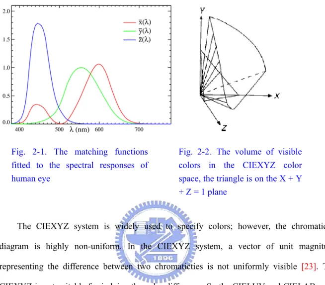
(25) device-independent color space, the same set of tri-stimulus values produces the same visual color on two different devices at the same viewing condition. As mentioned earlier, the color reproduction prefers to perform in the device-independent color spaces. The various device-independent color spaces are introduced in the following section.. 2.1.1 CIEXYZ color space In 1931, the CIE agreed on a device-independent standard color space called CIEXYZ, which was created in the need for describing colors in the mathematical equivalent way. The color was measured with tristimulus filters corresponding to the sensitivities of the receptors in the standard observer. The result was the functions of matching curves fitted to the detected wavelengths, as shown in Fig. 2-1. Then, the integrations of matching function multiplying the object and illumination reflectance were computed as tristimulus values: X, Y and Z. However, the tristimulus values were virtual tristimulus, and describing color in the three dimensions was not convenient. A derived color space specified by x, y, and Y was known as the CIE xyY color space. As shown in Fig. 2-2, the x and y is the coordinate of specific color on X + Y + Z = 1 plane by using the following equations: [22]. X X+Y+Z Y y= X+Y+Z Z z= X+Y+Z. x=. (2- 1). The third coordinate, z, can be omitted by providing Y parameter which is a measure of the luminance of a color. As a result, the chromaticity description of any color by using just two coordinates on the projecting locus of that plane, the CIE xy chromaticity diagram, is widely used in practice.. 14.

(26) Fig. 2- 1. The matching functions fitted to the spectral responses of human eye. Fig. 2-2 . The volume of visible colors in the CIEXYZ color space, the triangle is on the X + Y + Z = 1 plane. 2. 1. The CIEXYZ system is widely used to specify colors; however, the chromaticity diagram is highly non-uniform. In the CIEXYZ system, a vector of unit magnitude representing the difference between two chromaticties is not uniformly visible [23]. The CIEXYZ is not suitable for judging the color difference. So the CIELUV and CIELAB color spaces were developed for solving this problem.. 2.1.2 CIELUV color space The CIE 1960 u’,v’ (UCS) diagram was the first determined by the linear transformation of Yxy, in an attempt to produce a chromaticity diagrams, in which a vector of unit magnitude difference is equally visible at all colors as shown in Fig 2-3. Y is unchanged from XYZ or Yxy. The non-uniformity is reduced considerably, but the uniform brightness scale is not included.. 15.

(27) Fig. 2-3. The 1976 u’v’ chromaticity diagram and its color difference diagram Base on the CIE 1960 u’v’ diagram, the CIE developed the CIE 1976 UCS diagram transformed from Yxy and defined the CIE 1976 L*u*v*(CIELUV) space involves the uniform lightness scale. The transform was given by. ⎛Y ⎞ L* = 116 f ⎜ ⎟ − 16 ⎝ Yn ⎠. (2- 2). ⎧u * = 13L* (u '− un ') ⎨ * * ⎩ v = 13L (u '− un '). (2- 3). ⎧ f (k ) = 3 k if k > 0.08856 ⎪ ⎨ 16 if k ≤ 0.08856 ⎪ f (k ) = 7.87 k + 116 ⎩. (2- 4). 4X ⎧ ⎪⎪u ' = X + 15Y + 3Z ⎨ 9Y ⎪v ' = ⎪⎩ X + 15Y + 3Z. (2- 5). where. 16.

(28) 4Xn ⎧ = u ' n ⎪ X n + 15Yn + 3Z n ⎪ ⎨ 9Yn ⎪v ' = n ⎪⎩ X n + 15Yn + 3Z n. (2- 6). where Xn, Yn, and Zn are the tristimulus of the reference white. The u’ and v’ are the chromaticity coordinates of stimulus, the u’n and v’n are the chromaticity coordinates of reference white.. 2.1.3 CIELAB color space The CIE 1976 L*a*b* color space, abbreviated CIELAB, is another uniform color space that transformed from CIEXYZ color space and related to Munsell color system. Three color values L* (lightness), a* (red-green axis), b* (yellow-blue axis) calculated from the CIE tristimulus values. As shown in the follows:. L* = 116 f (. Y ) − 16 Yn. (2- 7). X Y ⎧ * ⎪ a = 500[ f ( X ) − f ( Y )] ⎪ n n for ⎨ Y Z * ⎪ b = 200[ f ( ) − f ( )] ⎪⎩ Yn Zn ⎧ f (k ) = 3 k if k > 0.08856 ⎪ ⎨ 16 f k ≤ 0.08856 ⎪ f (k ) = 7.87 k + 116 ⎩. (2- 8). where Xn, Yn and Zn are also the tristimulus values for the reference white, and L* ranges from 0 to 100, where 0 is perfect black, and 100 is the reference white. The counterclockwise angle between the positive a* axis and the vector from the origin to the color is referred to as hue angle. Hue angle hab and chroma C*ab are defined as follows:. 17.

(29) b* hab = arctan( * ) a C *ab = ( a*2 + b*2 ). (2- 9). The CIELAB color difference ΔE*ab between two points is calculated as the Euclidean distance:. ΔΕ*ab = (ΔL*2 + Δa*2 + Δb*2 ). (2-10). Since the CIELAB is the uniform device-independent color space, the color gamut and the gamut mapping process usually represent in the CIELAB space.. 2.2 Previous work - Wen’s method Although many of multi-primary displays were proposed for wider gamut representation, there were only few papers discussed its color gamut design and method. As previous noted, the shape and volume of device gamut will affect the color reproducibility. In addition, the MPDs offer the flexibility to adjust and exhibit possible CGV, and need the constraint to overcome the color conversion. So a previous method for design the relative luminance of four-primary display to decide its color gamut was proposed by Wen [24]. Wen had proposed two criteria to solve this problem, one was the Maximum White Point Luminance (display luminance) requirement, and the other was Maximum CGV requirement. Both of them were base on the basic white point requirement. A four-primary display was taken an example for showing the methods; it is the same condition with this thesis. For the maximum white point luminance requirement, first of all, the gamut setting was basically meeting the white point of the choosing system. For conventional three primary displays, the relative luminances of primaries were uniquely determined by the white point of display [25]. Utilizing the Grassman’s law, the white point tristimulus are the linear 18.

(30) combination of three primaries; the forward model refers to Eq. (1- 1) can be represented as follows:. ⎡Xw⎤ ⎡XR ⎢Y ⎥ = ⎢Y ⎢ w⎥ ⎢ R ⎢⎣ Z w ⎥⎦ ⎢⎣ Z R. XG YG ZG. X B ⎤ ⎡R⎤ YB ⎥⎥ ⎢⎢G ⎥⎥ Z B ⎥⎦ ⎢⎣ B ⎥⎦. (2-11). and refer to Eq. (1- 2) the relative luminance can be calculated by the backward model:. ⎡ xr ⎡ R ⎤ ⎢ yr ⎢G ⎥ = ⎢ 1 ⎢ ⎥ ⎢ ⎢⎣ B ⎥⎦ ⎢ zr ⎣ yr. xg yg. 1 zg yg. ⎤ ⎥ 1⎥ ⎥ zb yb ⎥ ⎦. xb yb. −1. ⎡ xyw ⎤ ⎢ w⎥ ⎢1⎥ ⎢ zw ⎥ ⎢⎣ yw ⎥⎦. (2-12). where (xr,yr), (xg,yg), and (xb,yb) are the color coordinates of red, green, and blue primaries; and (xw,yw) is the color coordinate of white point. For the four-primary LED display which Wen used, the additive fourth color is yellowish-green, which is denoted in Gy, enlarging the gamut about 130% NTSC in 1931 CIE xy chromaticity diagram and 137% NTSC in CIE 1976 uniform chromaticity scale (UCS) diagram. To achieve the white point, the forward model refers to Eq. (1- 3) as shown following:. ⎡Xw⎤ ⎡XR ⎢Y ⎥ = ⎢Y ⎢ w⎥ ⎢ R ⎢⎣ Z w ⎥⎦ ⎢⎣ Z R. XG YG ZG. ⎡R⎤ XB Xy ⎤ ⎢ ⎥ ⎥ G YB Yy ⎥ ⎢ ⎥ ⎢B⎥ Z B Z y ⎥⎦ ⎢ ⎥ ⎣⎢Gy ⎦⎥. (2-13). As previous noted, the backward model of four-primary in Eq. (2-13) can not be calculated. For solving the linear equations, there must add some constraint to reduce the. 19.

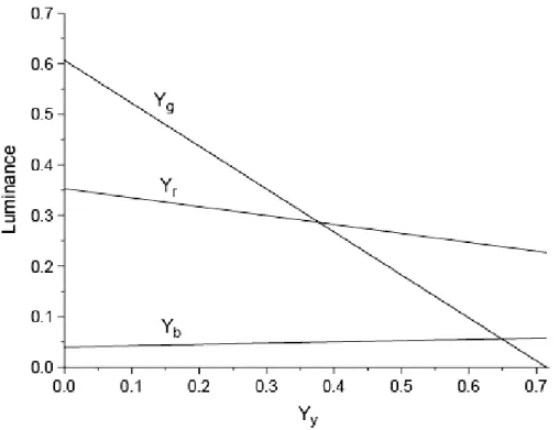
(31) column of matrix. As the definition of white point is the equal energy of each primary, it can be achieved by the R=B=G=Gy setting, where the normalized white point luminance is the sum of four primaries, as shown following:. Yr + Yg + Yb + Yy = Yw = 1. (2-14). where 0 ≤ Yr , Yg , Yb , Yy ≤ 1 , and Yr, Yg, Yb, Yy are the relative luminances of each primary. Furthermore, the simple tristimulus derived formula as shown following.. Z=. (1 − x − y ) x Y , X= Y y y. (2-15). As Eqs. (2-14) and (2-15) were applied for Eq. (2-13), the basic color conversion can get the backward model of relative luminance of four primaries: ⎡ xr ⎡Yr ⎤ ⎢ yr ⎢Y ⎥ = ⎢ 1 ⎢ g⎥ ⎢ ⎢⎣Yb ⎥⎦ ⎢ zr ⎣ yr. xg yg. 1 zg yg. ⎤ ⎥ 1⎥ ⎥ zb yb ⎥ ⎦. xb yb. −1. ⎡ xw − x y Yy ⎤ ⎢ yw y y ⎥ ⎢ 1 − Yy ⎥ ⎢z ⎥ x ⎢ yww − yyy Yy ⎥ ⎣ ⎦. (2-16). From Eq. (2-16), Yr, Yg, and Yb are dependent on linear function of Yy. The plotted curve of Yr, Yg, and Yb against Yy by increasing Yy, is shown in Fig. 2-4. The figure depicts that each combination of vertical line agrees with the white point setting, and the combination reduce to three primaries, when Yy at 0 and 0.715.. 20.

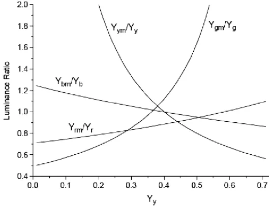
(32) Fig. 2-4. Luminance Yr, Yg, and Yb plotted against Yy under the white point requirement (S. Wen, Displays, 26, pp. 171-176, 2005). In addition, the requirement of the maximum display luminance is taken for a set of available primary luminances. Considering the available luminance of each LED Yrm, Ygm, Ybm, and Yym, the white point is satisfied when the. ar Yrm a g Ygm abYbm a yYym = = = =η Yr Yg Yb Yy. where 0 ≤ ar , ag , ab , a y ≤ 1 ,. Yim =. (2-17). Max luminance i k. ∑. i = r , g , b, y (2-18). Max luminance k. r , g ,b , y. In Eq. (2-17), ar, ag, ab, and ay are the turning factor of red, green, blue, and yellowish-green primaries. To meet the maximum efficiency, the desired ηis preferred as large as it can be. Therefore, the designed maximum efficiency of four LEDs ηmax is defined as. 21.

(33) ⎧⎪ Yrm Ygm Ybm Yym ⎫⎪ = = = ⎬ Yg Yb Yy ⎪⎭ ⎪⎩ Yr. ηmax (Yy ) = Min ⎨. (2-19). where Min { } is the minimum function. By using Eqs. (2-16) and (2-19), the changed relative luminance of yellowish-green Yy can get the curve plotted in Fig. 2-5 from which the maximum efficiency ηmax of 0.908 at Yy=0.44 can be derived. Thus, the initial four-primary color gamut with maximum white point luminance requirement is defined, when Yy=0.44, Yr=0.3, Yg=0.24, and Yb=0.05, respectively.. Fig. 2-5. Luminance ratios Yrm/Yr, Ygm/Yg, Ybm/Yb, and Yym/Yy plotted against Yy (S. Wen, Displays, 26, pp. 171-176, 2005) For the maximum CGV requirement, the gamut volume is present in the CIE Lab color space. By matching the white point setting, utilizing Eq. (2-16), the color gamut can be designed by the relative luminances of four-primary. In addition, the CGV can be calculated by the equation: CGV = ∫∫∫ G ( L* , a* , b* )dL*da*db* 22. (2-20).

(34) The color gamut volume is calculated in CIELAB color space when changing Yc value, which is plotted in Fig. 2-6 from which the maximum gamut volume of 1.61×106 at Yy =0.37 can be derived.. Fig. 2-6. The CGV (ΔΕ*ab3) of four-primary display plotted against Yy (S. Wen, Displays, 26, pp. 171-176, 2005) With these two proposed criteria, the four-primary display gamut can be achieved for its preferred application. Since the two criteria have two different settings, finally, Wen concluded that, in practice, the design of the relative primary luminances may be a compromised result of the two additional requirements. However, the criteria perform the largest CGV and maximum display luminance, but they do not consider the input CGV. So it may be not a suitable design for color reproduction.. 2.3 Proposed method Although the larger CGV can yield more colors, the mapping with input encoded CGV is 23.

(35) another key factor affecting the display color reproduction performance. Some paper [26] provides the metrics to judge the gamut volume of display, which depicts that the gamut volume characteristics is judged with the input encoding CGV. With this concept, the proposed new criterion is taking the input color gamut into account, which is the maximum intersectional CGV. Consequently, this thesis refers to the Wen’s method, with the maximum white point luminance requirement and adds the maximum input CGV intersection requirement. The method of designing the four-primary color gamut for reproducing maximum input encoded color was proposed. It compromised with the efficiency of maximum luminance, and performed the best gamut mapping resulted from input signal. A four-primary-LED backlight in FS-FC LCDs was constructed to verify the proposed method, will be introduced in next chapter. The four primaries are red, green, blue, and cyan, denoted in R, G, B, and C separately. To meet the white point, the forward model modified from Eq. (2-13) is shown as follows:. ⎡Xw⎤ ⎡XR ⎢Y ⎥ = ⎢Y ⎢ w⎥ ⎢ R ⎢⎣ Z w ⎥⎦ ⎢⎣ Z R. XG YG ZG. ⎡R⎤ X B XC ⎤ ⎢ ⎥ G YB YC ⎥⎥ ⎢ ⎥ ⎢B⎥ Z B Z C ⎥⎦ ⎢ ⎥ ⎣C ⎦. (2-21). The backward model of the relative luminance of four primaries modified from Eq. (2-16) is shown as follows: ⎡ xr ⎡Yr ⎤ ⎢ yr ⎢Y ⎥ = ⎢ 1 ⎢ g⎥ ⎢ ⎢⎣Yb ⎥⎦ ⎢ zr ⎣ yr. xg yg. 1 zg yg. ⎤ ⎥ 1⎥ ⎥ zb yb ⎥ ⎦. xb yb. −1. ⎡ xyw − xyc Yc ⎤ ⎢ w c ⎥ ⎢ 1 − Yc ⎥ ⎢ zw xc ⎥ − Y ⎣⎢ yw yc c ⎦⎥. (2-22). In addition, to consider the available luminance of each LED Yrm, Ygm, Ybm, and Ycm, the designed maximum efficiency of four LEDs, η max, modified from Eq. (2-19) is defined as: 24.

(36) ⎧⎪ Yrm Ygm Ybm Ycm ⎫⎪ = = = ⎬ Yg Yb Yc ⎪⎭ ⎩⎪ Yr. ηmax (Yc ) = Min ⎨. (2-23). According to the calculated result of Eqs. (2-22) and (2-23), the maximum white point requirement can be achieved by the specific relative luminance of four primaries. The proposed maximum input CGV intersection requirement which is calculating the CGV intersection with input CGV in the CIELAB color space. The test input CGV, the sRGB color space [27] and the “real world surface color” gamut by pointer [28], will be introduced in next section. Then, the 3D color gamut visualization and the intersectional CGV calculating simulation will be introduced in next chapter. In summary, the design flow of proposed method is shown in Fig. 2-7. First, the measurement data of four-primary color should be made to build a color database. Then, start designing the relative luminance of each primary. The first step is to meet the basic white point requirement by referring to the input color white point. Second, consult with the measurement database, the maximum available ratio also be calculated. With the maximum white point luminance design, the initial four-primary CGV can be determined by the relative luminance setting. Finally, the input CGV is taken to compare with the initial four-primary CGV. The maximum intersectional CGV will be found by shift-adjusting the initial setting. As a result, the new relative luminance setting decides the final four-primary CGV.. 25.

(37) no. Yes. Fig. 2-7. The design flow of proposed method. 26.

(38) 2.4 Test input color gamuts For the requirement of maximum input CGV intersection, the test color gamuts here, are the standard RGB (sRGB) color space and the “real world surface color”. The sRGB adopt the HDTV standard and is widely used in most monitor gamut management. Furthermore, the real surface database collected by pointer contains most of the colors that people can see in the real world.. 2.4.1 Standard RGB color space (sRGB) In 1996, Hewlett-Packard and Microsoft proposed a standard color space, sRGB, for the usage on monitors, printers, and the Internet. The aim of this color space was to complement the current color management strategies by enabling a third method of handling color in the operating system and device drivers. The sRGB is a single default color space acting as a bridge provides the good quality and backward compatibility with unambiguous and efficient transmission. Nowadays, the sRGB color space has been standardized by the International Electrotechnical Commission (IEC) as IEC 61966-2-1 in 1999 [29]. Such a standard can dramatically improve the color fidelity in the desktop environment The three major factors of the sRGB standard are the colorimetric RGB definition, the equivalent gamma value of 2.2 and the well-defined viewing conditions, along with a number of secondary details necessary to enable the clear and unambiguous communication of color. The sRGB standard used the ITU-R BT.709-2 reference primaries and the CIE standard illuminant D65 reference white. The ITU-R BT.709-2 defined the parameter values of the HDTV standards for production and international program exchange. The primaries and reference white of sRGB standard are given in Table 2-1.. 27.

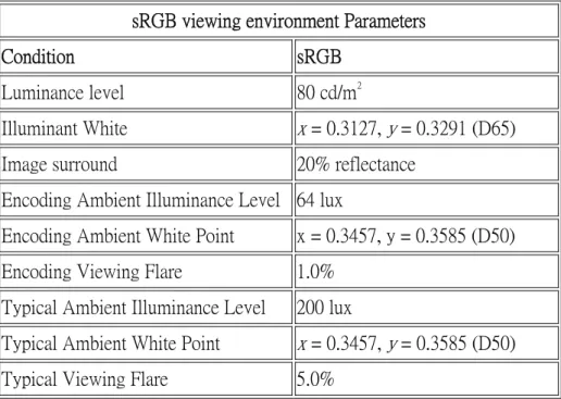
(39) Table 2-1 Parameters of sRGB chromaticties CIE chromaticities for ITU-R BT.709 reference primaries and CIE standard illuminant Red. Green. Blue. D65. x. 0.6400. 0.3000. 0.1500. 0.3127. y. 0.3300. 0.6000. 0.0600. 0.3290. z. 0.0300. 0.1000. 0.7900. 0.3583. Additionally, the standard adopted the transfer function (gamma 2.2) of typical CRTs. Gamma is the non-linearity of the electro-optical radiation transfer function of CRTs; This transfer function describes how much luminance results from voltages applied to the CRT, and often expressed by a mathematical exponential power function parameter. After defining the parameters of colorimetry, the sRGB color space is designed to match typical home and office viewing conditions rather than the darker environment typically used for commercial color matching. The viewing environment descriptions contain all the necessary information to provide conversions between the standard and target viewing environments, as shown in Table 2-2: Table 2-2 Parameters of sRGB viewing environment sRGB viewing environment Parameters Condition. sRGB. Luminance level. 80 cd/m2. Illuminant White. x = 0.3127, y = 0.3291 (D65). Image surround. 20% reflectance. Encoding Ambient Illuminance Level 64 lux Encoding Ambient White Point. x = 0.3457, y = 0.3585 (D50). Encoding Viewing Flare. 1.0%. Typical Ambient Illuminance Level. 200 lux. Typical Ambient White Point. x = 0.3457, y = 0.3585 (D50). Typical Viewing Flare. 5.0%. 28.

(40) 2.4.2 Real-world surface colors gamut In 1980, Pointer published an article titled “the gamut of real surface colours”, which collected 4089 measured surface color patches data enclosing most of the color in the real world. In this article all the data have been calculated using CIE Standard Illuminant C. The color patches contained the follows: (1) Munsell Color-Cascade (non-fluorescent) (2) Surface color objects measured by Trussel (3) DuPont paint samples (4) Graphic arts spot colors As show in Fig. 2-8, the measurement color data was plotted in the CIE1931 xy chromaticity diagram. In addition, the data were converted into CIELAB coordinates, sorted into groups according to the hue angle, hab, and then represented as plots of lightness, L*, as a function of chroma, Cab*. Similar calculations were made using the equivalent CIELUV coordinates. Both of these two coordinates collection used the convex hull, the smallest polygon that enclosed the sets of data to surround all these color data as a real-world surface color gamut.. 29.

(41) Fig. 2-8 The Pointer color gamut in CIE xy chromaticity diagram. This thesis used the sRGB and real-world surface color gamut in the CIELAB coordinate as input colors to evaluate the CGV setting of the four-primary LED backlight. Therefore, through the quantitatively evaluation of two input color gamuts, the four-primary gamut was able to represent the color chart with as much color fidelity as possible.. 30.

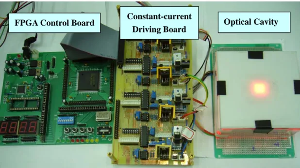
(42) Chapter 3. Experiment and Simulation This chapter has been divided into two sections: experiment and simulation. The experiment section includes four-primary-LED backlight platform, measurement equipment, and the measurement data, which will be firstly described for establishing a color database. In the simulation section, the simulation method for evaluating the gamut characteristic will be described.. 3.1 Experiment In this section, a four-primary-LED backlight in FS-FC LCDs has been constructed to verify the proposed method. The related measurement equipment and measurement data would be shown later.. 3.1.1 Four-primary-LED backlight platform The four-primary-LED backlight platform, as shown in Fig. 3-1, was composed of an optical cavity, a constant-current driving board, and a Field-programmable gate array (FPGA) control board. These parts would be introduced separately.. 31.

(43) FPGA Control Board. Constant-current Driving Board. Optical Cavity. Fig. 3-1. The photo of four-primary-LED backlight platform, which included (a) a optical cavity, (b) a constant-current driving board, and (c) FPGA control signal board. The optical cavity, a sample of LED-Direct-Backlight, which was composed of four high flux LEDs i.e. Luxeon Star LEDs. A set of diffusers were coverd on the four LEDs cavity. The main target was to mix the four-primary colors to obtain the best brightness and color uniformity in the center of the diffusers. The optical cavity and specifications of the selected LEDs from LUMINLEDS Corporation are shown in Fig. 3-2, where the peak wavelengths of red, green, blue, and cyan primaries were 625nm, 530nm, 470nm, and 505nm, respectively.. Fig. 3-2. The photo of simple optical cavity and the correlative specification of LED. 32.

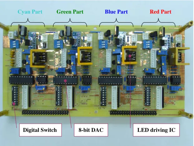
(44) The constant-current driving board designed to provide the constant current for each LED was expecting for the uniform color mixing result. As shown in Fig. 3-3, the circuit board was divided into four similar parts, and each part deriving one specific LED. The digital switch monitored the current which drives the LEDs, and the digital values were coded on eight bits digital/analog converter (DAC) resulting in 256 digital values. Moreover, the other circuits aided the LED driving IC providing different constant currents by the setting of each digit count.. Cyan Part. Green Part. Digital Switch. Blue Part. 8-bit DAC. Red Part. LED driving IC. Fig. 3-3. The photo of constant-current driving board and its description The FPGA control board produced the time-sequential signal allowing the switching of the driving current for each LED. This board was connected to the electronic driving board. By the Verilog coding, the digital count and the timing signal has been provided for each LED.. 33.

(45) 3.1.2 Measurement equipment The instrument used to realize the measurements was the Conoscope, as shown in Fig. 3-4. The Conoscope has different applications: luminance vs. viewing direction, chromaticity vs. viewing direction, response time, flicker-analysis, lateral homogeneity, interactive viewing cone analysis, and electro-optical characterization, etc.. Fig. 3-4. The photo of Conoscope. In this thesis, the interesting function is the ability of the Conoscope to realize the measurements of the color coordinates (x, y) and tristimulus on our sample backlight. In the Conoscope, the luminous information of measurement sample is sent to two different devices, as shown in Fig. 3-5, totally independent in their work. The first device is the photometer with the CCD camera, which allows the measurement of the color coordinates. The results of the experiments are displayed on the computer linked to the Conoscope. The second device is the spectrometer, which provides more accurate spectrum measurement. The main function of the spectrometer is to measure the wavelength of the light produced by the studied sample. Additionally, the tristimulus and CIE coordinates was calculated by this function. 34.

(46) Photometer +CCD. Spectrometer. Fig. 3-5. The luminous information path in Conoscope. The Conoscope is based on the conoscopic method. As shown in Fig. 3-6, a cone of elementary parallel light beams C, which is transmitted by a sample S that is located in the front of focal plane of the lens L1, is collected simultaneously over a large solid angle by the lens L1. A pattern IF1 is generated in the rear focal plane F’1 of the lens L1 by the transform lens. The intensity of each area element corresponds to the intensity of one elementary parallel beam with a specific direction of light propagation. In the pattern IF1, the directional intensity distribution of the cone of elementary parallel light beams C is transformed into a two-dimensional distribution of light intensity and color with each location in the pattern corresponding to exactly one direction of light propagation (θ, ψ). For the CCD detector, a second optical system L2 optionally projects the conoscopic figure IF1 on a two dimensional detector array for evaluation of the spatial intensity distribution, which corresponds to the directional intensity distribution of the light emerging from the measuring spot on the sample.. 35.

(47) Fig. 3-6. The principle diagram of Conoscope. 3.1.3 Measurement data The specifications of each LED were measured by Conoscope Spectrometer. The calculated color gamut was about 131% of NTSC color gamut in 1931 CIE xy chromaticity diagram and 147% of NTSC color gamut in CIE 1976 UCS diagram, as shown in Table 3-1.. Table 3-1 LED specifications and measurement data. LED Spec. Part num. Color LXHL-MD1D Red LXHL-MM1D Green LXHL-MB1D Blue LXHL-ME1D Cyan. Measurement Data Calculate Data x y 0.70 0.30 CIE xy 131% 0.16 0.71 color gamut NTSC. Peak λ 625 nm 530 nm 470 nm 505 nm. 0.14 0.08. 0.05 CIE u'v' 0.54 color gamut. 147% NTSC. The four-primary color gamut compared to other standard color gamuts in CIE 1976 UCS diagram is shown in Fig. 3-7 from which the designed color gamut was sufficient to reproduce the standard color gamut input.. 36.

(48) CIE 1976 uniform chromaticity scale diagram 0.6 0.5. v'. 0.4 0.3 0.2. Four-primary NTSC sRGB D65. 0.1 0.0 0.0. 0.1. 0.2. 0.3. 0.4. 0.5. 0.6. u' Fig. 3-7. Four-primary color gamut compared with standard color space in CIE 1976 UCS diagram In addition, the database of these LEDs was measured by the adjustable current driving circuit, as shown in Fig. 3-8. The luminances of four LEDs, which denoted in R, G, B, and C, are almost linear functions of the digital count. The measurement data are also plotted in CIE 1931 chromaticity diagram, as shown in Fig. 3-9. The coordinates are not varied with the digital count. Therefore, the database of these LEDs can be applied to the color gamut evaluation. 2000 1800. Digital count vs. Luminance. 1600. G. Luminance. 1400 1200 1000. R. 800 600. C. 400. B. 200 0 0. 32. 64. 96. 128 160 Digital Count. 192. 224. 256. 280. Fig. 3-8. Luminance of each primary plotted against digital count of control circuit 37.

(49) CIE 1931 xy chromaticity diagram 0.9 0.8 0.7 0.6 0.5 y 0.4 0.3 0.2 0.1 0.0 0.0. 0.1. 0.2. 0.3. 0.4. 255 gray level. .. 0.5. 0.6. 0.7. 0.8. 0 gray level. Fig. 3-9. The plot of different digital count (dived in to 8 level) in the CIE xy chromaticity diagram. 38.

(50) 3.2 Simulation The simulation includes the analysis of numerical parameters that above mentioned and the gamut visualization in three dimensions performed to observe the gamut intersection. In addition, the q-hull algorithm was also introduced in this section.. 3.2.1 Numerical analysis There are several parameters need to be simulated, included the max efficiency ηmax , maximum four-primary CGV, and the intersectional CGV (with input color gamut). As mentioned before, the four-primary would produce a set of combinations through different relative luminance setting. Therefore, the max efficiency ηmax was calculated by satisfying Eqs. (2-22) and (2-23). The maximum four-primary CGV and the intersectional CGV of four primaries and test input colors were calculated by Eq. (2-20), and both of them try to meet the maximum values by adjusting the relative luminance.. 3.2.2 Gamut visualization As mentioned earlier, the color gamut is usually visualized and processed in the CIELAB color space. Because there are lots of set colors, the visualization of the gamut volume should use a convex hull to enclose all these data. The convex hull is the smallest polygon that enclosing all sets of data. As shown in Fig. 3-10, the set of color data in CIELAB color space are denoted, S, and the convex hull is the set which contain all the data denoted, CH(S). There are many algorithms for solving the convex hull problem. This thesis used the q-hull algorithm for the high speed approach, and it would be introduced later.. 39.

(51) L*. b*. a* Output: CH(S). Input: S. Fig. 3-10. The concept of convex hull in gamut visualization. 3.2.3 Q-hull algorithm The q-hull algorithm is the abbreviation of quick hull, which can provide the fast process in practice. The method is similar to the quick sort algorithm, the average time complexity is O (n log n). The simple illustration of q-hull algorithm method is shown in Fig. 3-11. There are a set of points in the diagram. First, two points P1 and P2 are chosen and a line is drawn dividing the set of points in two parts i.e. X1, X2. In X1 part, the P3 is chosen to compose of the largest triangle area of P1P2P3. Further, keep doing the same procedure, in the end; the final convex hull will be given.. Fig. 3-11. The simple illustration of q-hull algorithm method. 40.

(52) Chapter 4. Results & Discussion The simulations of two input color gamuts, sRGB and real surface color gamut, are demonstrated and compared with the experimental data. Two commonly considered criteria and our proposed one will be examined in both input cases. These criteria include maximum white point luminance, maximum four-primary CGV and maximum intersectional CGV. The CGV is calculated in CIELAB space and depicted in three dimensions for direct comparison and clear visualization.. 4.1 sRGB color gamut as the input The input color gamut is sRGB color space, which was introduced in section 2.4.1, and the results from fulfilling of the three criteria will be shown separately.. 4.1.1 Maximum white point luminance The white point and the maximum available luminance of LEDs are required to meet the maximum white point luminance as proposed by Wen. For a standard ITU-R BT.709 (sRGB) input encoded color signal, the white point D65 decided by the maximum luminance and relative ratio of each primary is the starting point for defining the color gamut of a display. Using the measured database and Eq. (2-22), the white point shown in Table 2-1 can be achieved by different combinations of relative luminance setting. The varied Yc was applied to Eq. (2-22), and plotted curve, as shown in Fig. 4-1, was resulted. Each vertical line in the diagram is under the white point requirement, e.g. when the relative luminance is setting at. 41.

(53) vertical line 1, which is Yc=0.2, Yr=0.289, Yg=0.45, and Yb=0.061, the mixing result will agree with the D65 white point coordinates. It is noticed that the LED backlight reduces to three primaries for the cases of Yc= 0 and 0.63. Because Yc is the luminance of comprises of blue and green spectral components, the required luminance of blue and green primaries decrease as Yc increases. On the other hand, the required luminance of red primary is increased with Yc. Therefore, the varied Yc lies on the range of two boundaries.. 0.7 Vertical Line1. 0.6. Luminance. 0.5. Yg. 0.4 Yr. 0.3 0.2 0.1 0 0. Yb. 0.1. 0.2. X: 0.63 Y: 0.007043. 0.3. 0.4 Yc. 0.5. 0.6. 0.7. Fig. 4-1. Plots of luminances Yr, Yg, and Yb as functions of Yc under the white point requirement In addition, if considered the available luminance ratio of each LED at the white point, the luminance ratios as functions of Yc are shown in Fig. 4-2 by Eqs. (2-22) and (2-23). The minimum ratio is 0.9801 at Yc=0.2 which is the maximum efficiency. ηmax defined by Eq.. (2-23). The designed efficiency of four LEDs η is plotted in Fig. 4-3 by applying the varied Yc to Eq. (2-23) for the comparison. As shown in Fig. 4-3, the maximum efficiency of 0.98 at Yc=0.2 can be derived. Therefore, the initial four-primary color gamut with maximum white point luminance requirement is defined, when Yc=0.2, Yr=0.289, Yg=0.45, and Yb=0.061, respectively. 42.

(54) 1.8 1.6. Luminance Ratio. 1.4. Ybm/Yb. 1.2 1 X: 0.2 Y: 0.9801. 0.8. Yrm/Yr. Ygm/Yg 0.6 0.4. Ycm/Yc. 0.2 0 0. 0.1. 0.2. 0.3 Yc. 0.4. 0.5. 0.6. Fig. 4-2. Plots of luminance ratios Yrm/Yr, Ygm/Yg, Ybm/Yb, and Ycm/Yc as functions of Yc under the white point requirement 1.0. M a x efficiency. 0.9. Efficiency. 0.8 0.7 0.6 0.5 0.4 0.20 0.3. 0.0. 0.1. 0.2. 0.3 Yc. 0.4. 0.5. 0.6. Fig. 4-3. The available LED efficiency plotted against Yc under the sRGB gamut input. 4.1.2 Maximum four-primary CGV The maximum CGV of four-primary display was also considered in Wen’s method. The CGV was calculated in CIELAB color space by Eq. (2-20) with the varied Yc value, as shown 43.

(55) in Fig. 4-4. The maximum gamut volume of 1.7×106 at Yc=0.24 can be derived. As a result, the maximum four-primary CGV with white point requirement is defined, when Yc=0.24, Yr=0.291, Yg=0.409, and Yb=0.06, respectively. 6. 3. Four-primar CGV (ΔΕab ). 1.74x10. Max CGV. 1.67x10. 6. 1.61x10. 6. 1.55x10. 6. 0.0. 0.24 0.1. 0.2. 0.3. 0.4. 0.5. Yc. Fig. 4-4. The four-primary CGV plotted against Yc under the sRGB gamut input. 4.1.3 Maximum input CGV intersection According to the design flow of proposed method in Fig. 2-7, the initial four-primary CGV was achieved by fulfilling of the maximum white point luminance requirement. In addition, the initial four-primary CGV with different relative luminance setting was compared with the input gamut. Therefore, the intersectional CGV of four-primary LED backlight and sRGB color gamut was also derived by Eq. (2-20). Then, the intersectional CGV plotted against the shifted Yc value is shown in Fig. 4-5. Obviously, from this figure, the intersectional CGV value becomes larger when Yc value is reduced. The maximum value is achieved when the initial Yc value shift from 0.2 to 0.04. By using Eq. (2-22), the relative luminances are Yc=0.04, Yr=0.278, Yg=0.615, and Yb=0.067, respectively.. 44.

(56) Max Intersection. 5. 8.0x10. 5. Intersectional CGV. 7.5x10. 5. 7.0x10. 5. 6.5x10. 5. 6.0x10. 5. 5.5x10. shift 1.6. 5. 5.0x10. 5. 4.5x10. -2. -1. 0. 1. 2. 3. 4. Yc shifted value Fig. 4-5. Plot of intersectional CGV as a function of the shifted Yc value under sRGB gamut input. In order to observe the color gamut intersection, the 3D CGV visualization of initial four-primary and sRGB color gamut were presented in CIELAB color space by q-hull algorithm simulation, as shown in Figs. 4-6 and 4-7. Furthermore, the intersectional CGV visualization by combining the two color gamut is shown in Fig. 4-8 from which some part of sRGB CGV is not included in the four-primary CGV.. (a). (b). Fig. 4-6. 3D visualization of four-primary gamut in CIELAB color space with different angle of (a) top and (b) side view. 45.

(57) (a). (b). CGV=7.87+e5. Fig. 4-7. 3D visualization of sRGB color gamut in CIELAB color space with different angle of (a) top and (b) side view. Four-primary. sRGB. Fig. 4-8. 3D CGV Intersection of four-primary gamut and sRGB gamut. 4.1.4 Summary With sRGB color gamut as an input, the results of three criteria are performed by the value setting shown in Table 4-1. The relative luminance of each primary and the digital level setting were listed. Furthermore, the curves based on three criteria are plotted in Fig. 4-9 for the comparison.. 46.

(58) Table 4-1 The relative luminance setting of each criterion with sRGB gamut input Relative luminance Max White Point Ratio Luminance Level Ratio Max CGV Level The Proposed Ratio Design Level 100. Yr 0.289 255 0.291 220 0.278 180. Yg 0.45 254 0.409 197 0.615 255. Yb 0.061 209 0.06 175 0.067 168. Yc 0.2 248 0.24 255 0.04 36. Max intersectional CGV. Intersectional CGV. 95 90 85 80 75 70 65 0.3. 0.4. 0.5 6. 1.73x10. Max CGV 0.9. 6. 1.66x10. Efficiency. 0.8 0.7. 6. 1.60x10 0.6 0.5. 6. 1.54x10 0.04. 0.4 0.0. 0.1. 0.20. ). 0.2. 3. 0.1. Max efficiency. Four-primary CGV (ΔΕab. 0.0. 1.0. 0.24. 0.2. 0.3. 0.4. 0.5. Yc. Fig. 4-9. Efficiency, four-primary CGV, and the intersectional CGV plotted against Yc for comparison with sRGB gamut input The comparisons of computed data based on three criteria including the maximum efficiency, four-primary CGV, and intersectional CGV, are shown in Table 4-2. The first row is the computed results of maximum white point luminance requirement at Yc=0.22, the maximum efficiency is 0.98, the four-primary CGV is about 1.696 x 106, and the 47.