PATH PLANNING IN THE PRESENCE OF OBSTACLES BASED TASK REQUIREMENTS

Path Planning in

the

Presence

of

Obstacles Based

on

Task Requirements

...

. . .

Tzung-hsien Wu and Kuu-young Young* Department of Contvol Engineering Na f ional Chiao- Tung University Hsinchu 30039, Taiwan, R.O.C.

Received January 31, 1992; revised April 5, 1993,

accepted May 2, 1994

We propose a novel and efficient scheme for planning a kinematically feasible path in the presence of obstacles according to task requirements. By employing geometrical analysis, we derive expressions to describe the relationship between the planned path, kinematic constraints, and obstacles in the robot workspace. The freedom avail- able according to task requirements is then utilized to modify the infeasible portions of the planned path. We use a 6R (revolute) wrist-partitioned type of robot manipulator and a spherical obstacle as a case study to demonstrate the proposed scheme. We then extend our results to general wrist-partitioned types of robot manipulators and arbi- trarily-shaped or multiple obstacles. 0 2994 john wdey 6 Sons, Inc.

1. INTRODUCTION ferent constraints need to be satisfied, including

task specifications, the avoidance of obstacle; within the robot workspace, and the inherent limita- tions of the robot manipulator. These constraints are Robot trajectories are planned according to different

industrial tasks. To obtain feasible trajectories, dif-

*To whom all correspondence should be addressed. summarized in Table I-The task-level constraint arises

Journal of Robotic Systems 11(8), 703-716 (1994)

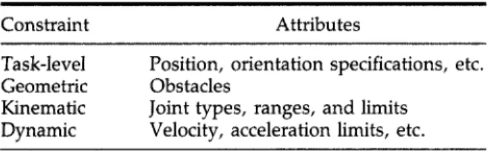
Table 1. Constraints for a feasible trajectory.

Constraint Attributes

Ta sk-level

Geometric Obstacles

Kinematic

Dynamic Velocity, acceleration limits, etc.

Position, orientation specifications, etc. Joint types, ranges, and limits

from different task requirements. For instance, if the task is to move a directionless object from one loca- tion to another, then only the starting and end posi- tions need to be considered, and the intermediate positions and orientations may be arbitrary. On the other hand, if the object to be moved is a cup of coffee, then the orientation specification also needs to be taken into account. The constraint due to the presence of obstacles inside the robot workspace, which is usually identified as the geometrical con- straint, is met by planning collision-free paths among obstac1es.l The kinematic constraint is due to joint types, ranges of motion, and other kinematic limitations of the robot manipulator used. Last, the dynamic constraint results from the velocity and ac- celeration limitations of the robot actuators. Plan- ning robot trajectories to meet these constraints gen- erally involves two steps: first, we find a feasible path that meets the task-level, geometric, and kine- matic constraints; second, we design a velocity pro- file along the planned path that satisfies the dy- namic constraints.2

The discussion in this article will focus on the first of the two stages just mentioned. There are several common approaches to planning a feasible path. One is to plan a path in Cartesian space by specifying both position and orientation for each

point on the The rationale for this approach

is that both position and orientation need to be spec- ified to find unique corresponding joint positions. The path planned by this approach tends to induce unnecessary infeasibility because extra constraints are imposed. Moreover, because knowledge of the kinematic constraints is not incorporated in the planning, kinematically infeasible paths cannot be modified and must be replanned. Even after replan- ning, the procedure is still one of trial-and-error, for the replanned path may still be infeasible.

Another approach to planning a feasible path is to search for a feasible path in the joint or configura- tion space according to the kinematic constraint or

obstacles. A famous method is the configuration

space (C-space) a p p r ~ a c h . ~ In the configuration

space approach, obstacles for a manipulator with n joints are formulated as C-space obstacles of n-di- mensional volume. To represent an n-dimensional C-space obstacle in C-space, the obstacle is recur- sively sliced into obstacles of fewer dimensions, un- til a union of onle-dimensional volumes is obtained, Feasible paths are then located by searching the free regions in tlhe configuration space to avoid ob- stacles and constraints from the kinematics. The main problem with this approach is the complexity of the C-space obstacle, especially when the dimen- sionality of the C-space is high. To reduce the com-

plexity of the C-space obstacle, in ref. 6 a sequential

search strategy was developed based on the as- sumption that tlhe motion of a proximal link does not depend on the motion of a distal link. One n- dimensional problem for an n-link manipulator arm

is reduced to an n - 1 two-dimensional planning

problem. However, this approach may not find a collision-free path in some cluttered environments even if one such path exists. In addition, mapping the task-level constraints in Cartesian space onto joint or configuration space is by no means an easy task.

We propose a novel and efficient approach, based on task requirements, to designing a kine- matically feasible path in the presence of obstacles. Instead of search.ing for a feasible path in the config- uration space, as, in ref. 5, we propose first to plan a path in a way similar to the approach in refs. 3 and

4, by specifying both position and orientation for

each point on the path. Then, according to different task requirements, we will modify the portions of the path that are infeasible due to kinematic con- straints and obstacles. As a result, a feasible path satisfying the task-level, geometrical, and kinematic constraints can be found in a smaller search space. To ensure that th.e modification part of our approach will succeed, we also develop representations of kinematic constraints and obstacles in the robot workspace and appropriate modification strategies. We use a geometrical approach to derive expres- sions that accurately describes the relationship be- tween the robot workspace and the planned ~ a t h . ~ , ~ Through this analysis, different geometrical regions corresponding to the kinematic constraints of the robot manipulator used and obstacles will be identi- fied in the robot workspace. For details on how to generate regions corresponding to kinematic con- straints inside the robot workspace, refer to ref. 9. A classification of inodification strategies correspond- ing to various task requirements can also be found

Wu and Young: Path Planning 705

cles inside the robot workspace are to be formulated and how modification strategies can be developed to cope with the presence of obstacles. We use the

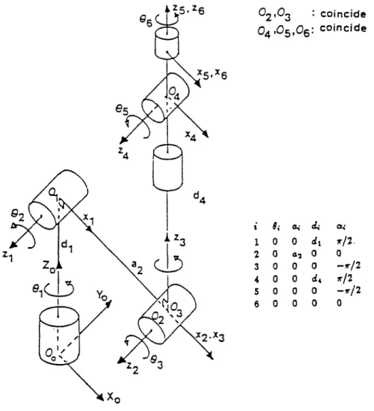
six revolute (R) joint wrist-partitioned type of robot

manipulator shown in Figure 1 and a spherical ob-

stacle as a case study. We then extend our results to general wrist-partitioned types of robot manipula- tors and arbitrarily-shaped or multiple obstacles. Simulations are performed to demonstrate the pro- posed schemes.

2. WORKSPACE ANALYSIS

The workspace of a robot manipulator can be sepa- rated into two parts: the positional and orientational

workspaces. A planned path is feasible if points on

the path are within the feasible regions of these two

workspaces. To take advantage of the wrist-parti- tioned structure of the 6R non-redundant robot ma- nipulator used in this study, we will select the wrist

position

1~~

space can be divided into the workspace of the wrist and that of the minor joints. There will then be two 3D (3-dimensional) workspaces to be analyzed in-

stead of a 6D workspace. consequently, 3D obsta-

cles can be easily formulated inside the workspaces. The positional workspace can be defined as that of the wrist constrained by the primary joints, de-

noted by PWK. Inside PWK, geometrical regions

corresponding to different kinematic constraints, such as feasible regions, areas of different configura- tions, and singular areas, can be determined. Here the feasible regions correspond to the joint variables within the joint ranges, the areas of different config- urations are defined as different sets of points with

i 8 ; s . h . cq' 3 0 0 0 - n p 5 0 0 0 -n/2 1 0 0 d t ~ / 2 . 2 0 a 2 0 0 4 0 0 d , r/2 6 0 0 0 0

the same arm configuration, and the singular areas are the vicinities of the boundaries of the feasible regions and positions where the corresponding joint variables are undefined.'O With these geometrical regions described in the robot workspace, the planned path can also be identified inside the work- space by mapping the sets of joint variables specify- ing the planned path onto corresponding traces in the regions. Using this geometrical approach, the mapping transforms the analysis of joint variables, represented numerically, into traces in the work-

spaces, represented geometrically. As a result, geo-

metric information related to kinematic constraints, obstacles, and neighboring points on the path in these workspaces can be derived.

It can be seen that each element within PWK

will not only determine a wrist position but also a wrist coordinate frame for mounting the minor

6.

0

- 2 -

-4 -

joints. Thus the orientational workspace, denoted

by OWK, consists of two parts: the orientational

workspace of the wrist as a function of the primary

joints, denoted by OWKP, and the orientational

workspace as a function of the minor joints, de-

noted by OWK". The feasible regions, areas of dif-

ferent configurations, and singular areas can all be

identified within OWK".

2.1. Positional Workspace

To identify OWK'" with three degrees of freedom (dof), we need to mount an end-effector with lengths in at least two different orientations upon the wrist.9 Without loss of generality, we may spec-

ify the end-effector to consist of two lengths, h, in

the ge direction and h, in the 0, direction. Using the lengths defined for the end-effector, we can derive

the wrist position

pm

end-effector's location, POS, as follows:

where

p e

ae]

Because the traces of links two and three due to the rotations of joints two and three are in the same plane in this case study, we need to further divide

the analysis of PWK into two subworkspaces: PWKl,

corresponding to joint one, and PWK23, correspond-

ing to joints two and three.

2.1.1. PWK, in the Presence of an Obstacle

The spherical obstacle, denoted by OBS, is specified

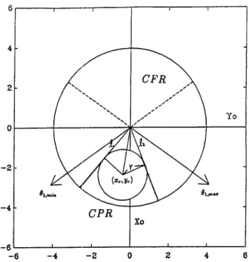
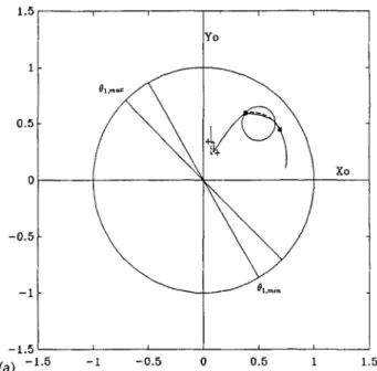
to be of radius r, with its center at (xr, yr, zr). PWKl -6

-6 -4 -2 0 2 4 6

Figure 2. Wo:rkspace of joint one with obstacle.

is divided into four regions of different configura-

tions by the lines corresponding to projections of

p.,

when joint one is at the maximum and mini-

mum (61,min) positions, re~pectively.~ By projecting

OBS onto the (xo, yo) plane, we can obtain PWKl in

the presence of O B S , as shown in Figure 2. Projec-

tions of OBS form a circle, OBS1, with radius r and

its center at (xr, yr). The slopes (tan

el)

lines tangential to OBS1,

el

e2,

mined by the following equation:

Using

el

t 2 ,

sion free region (CFR) and collision possible region (CPR), corresponding to the regions without and

with OBS1, respectively. OBS will not affect the fea- sibility of the projections of the wrist path within the

CFR. However, for projections within the CPR, it is

possible that the wrist may collide with the obstacle,

depending upon the feasibility analysis in PWKZ3.

2.1.2. PWKZ3 in the Presence of an Obstacle

To generate PW1<23, we derive

lpw(lx,,,

removing from

pw

joint one. Then iDWK23 can be obtained by rotating joints two and three from their minimums to maxi-

Wu and Young: Path Planning 707

-0.2

mums. Due to the geometries of joints two and

three, PWK23 depends not only on the limits of

e3

but also on its range. It takes four cases and five

circle equations to specify the boundaries of PWKZ3 .9

To analyze PWK23 in the presence of OBS, we

need to find the mapping of OBS on PWK23. We

propose slicing OBS by the planes containing the zo

axis and rotating the slices back to the (XI, yl) plane

of dl = 0, where PWK23 is located. Because OBS is a

sphere, the slices will contain circles with different radii. To avoid performing a separate analysis for each slice, we will choose the circle with the largest

radius rmax, OBS23, which covers all the others, as

the mapping of OBS on PWK23. The center of OBS23

is defined as (Ixr,

'yr).

means that we will be analyzing an obstacle that is

larger than OBS. This expanded obstacle is donut-

shaped. It can be seen that if a donut-shaped obsta-

cle with its circular side perpendicular to the (xl, yl)

plane is analyzed through the above procedure, it will turn out that we actually are not dealing with an expanded obstacle after all. This implies that a do- nut-shaped object may be a better representation of an obstacle than the spherical object used in this

approach. A further discussion of obstacle represen-

tation is in section 3.2.

Depending on the location of OBS23 in PWK23,

the path of link two will fall into one of three cases:

(a) Link two cannot reach OBS23; (b) Link two can

reach OBS23 and is tangential to it when contact oc-

curs; (c) Link two can reach OBS23 and is not tangen-

tial to it when contact occurs. In the following, we use case (a) as an example for demonstration; the other two cases can be tackled in a manner similar to

that used for case (a). Four circles, C1-C4, will be

employed in the analysis of case (a) (see Fig. 3):

C1: 'xf

+

+

e3,max

. .

- CI c2 c3 c4

where C1 and C3 represent the circles when joint two rotates throughout its range with joint three equal to

63,max and respectively; C2 the circle with ra-

dius equal to the length of link two u2; and C4 the

circle with radius u2

+

boundary of PWK23. In Figure 3, the portion of

PWK23 shown is in the middle range of 02, and it is assumed that

Illpwll <

II1pzL,ll

>

u2 when

e3

There are two kinds of configurations in PWK23,

elbow-flip (EF), and elbow-nonflip (ENF). With O3

specified to be -90" when links two and three are

along the same line, the EF configuration is obtained

when 6 3 E -90"], and ENF is obtained when

tI3

the presence of OBS23, the feasible region will be

reduced by the area not only of OBSz3 but also its

neighboring area.

To analyze how PWK23 is affected by OBS23, we

employ the end positions of links two and three, Pl(pl,, ply) and P z ( p z x , pzy). If we consider the ENF

configuration in Figure 3, curves Al and A2 are the

traces of P2 when link three is tangential to OBS23

from different sides. Curves A1 and A2 start from bl

and b2, where P2 contacts OBS23, and end when

links two and three are aligned along the same line.

The 62 and 63 corresponding to these curves can be

obtained as follows:

where u1 corresponds to O2 when P2 contacts OBS23

and u2 to 1 3 ~ when links two and three are aligned

configuration, curves A3 and A4 can also be ob-

tained, except that curve A4 will start from b5 instead

of b4, where b5 is the intersection of the tangential

curve and C3. With curves A1-A4, in Figure 3 the

area bounded by Al, A2, C4, and OBS23 cannot be

reached by the ENF configuration, while the area

bounded by A3, A4, C3, C4, and OBS23 cannot be

reached by the EF configuration. Based on the above analysis, four areas D1-D4 in PWK23 affected by the

presence of OBS23 can be identified: 0 1 becomes

only relevant to the ENF configuration; 0 2 becomes

only relevant to the EF configuration; and 0 3 and 0 4

are not feasible now.

2.2. Orientational Workspace

To analyze OWK, we employ the orientation Re =

[_ne CJ,

a,],

As indicated in Eq.

(€9,

dinate frame for mounting "Re. Because R, can be

determined after the analysis of

p w

fect of OWKP can be removed and "R, can be solved

from Consequently, the analysis of OWK be-

comes that of OWK". With the end-effector position

constrained by the limits and ranges of the minor joints, the analysis of OWK"' is equivalent to the positional feasibility analysis of the end-effectors9

The end-effector can be represented in the wrist

coordinates (x,

,

,

tions:

where "_n,, "gel and are the orientational vectors of "Re. In Figure 1, the workspace of "Iz, can be constrained only by the ranges and limits of joints

four and five. Therefore "_h, can be used to analyze

the workspaces of joints four and five. Because the rotations of these two joints are not about the same axis, two subworkspaces are formed corresponding

to joints four and five. The workspace swept by

,by,

on the other hand, is constrained by all three joints; however, after the analyses of the workspaces of joints four and five, their effects can be removed

and used to analyze the workspace of joint six

a10ne.~ In general, the end-effector is small com-

pared with the links corresponding to the major

joints. Therefore, to ensure that the presence of OBS

will not affect OWK", we propose expanding the

radius of OBS b'y all or a ortion of the length of

the end-effector,.

4

will depend on different modification strategies; we

will return to this problem in section 4.

3. EXTENSION TO GENERAL CASES

The analysis of the above case study can be ex- tended to (a) general wrist-partitioned types of ro- bot manipulators and (b) arbitrarily-shaped or mul- tiple obstacles.

3.1. General Wrist-Partitioned Types

of Robot Manipulators

To extend the results of the case study to general wrist-partitioned types of robot manipulators, we need to consider three major factors: offsets, pris- matic joints, and the different connections between the joints. First, the effect of offsets can be identified

as follows. For PWK23 of the case study, for exam-

ple, we assume that both offsets are present and that they are perpendicular and parallel to links two and three, respectively. If the traces of the links and offsets to the ( x l ,

yl)

about the zo axis and their projections are taken, the

projections of the offset perpendicular to the links will have no effect on the traces. The projections of the offset parallel to the links are stationary with respect to the links and can be viewed as parts of the links. The above reasoning can also be applied to PWKl. Thus, after the effect of the offsets is identi- fied, the proposed approach can also be utilized to analyze robot manipulators with offsets.

Second, it can be seen that workspace analyses involving prismatic joints are much simpler than

those involving revolute ones. This is because a

prismatic joint rnoves the link along a straight line, while a revolute joint moves it along a curve. Third, there are three non-redundant ways in which three major points may be connected: (a) last two joints in parallel, (b) first two joints in parallel, and (c) all three joints consecutively perpendicular. The first case is the same as that of the case study. The analy- sis of the second case will be similar to case (a) if it is performed by starting from the third joint, and then going on to the first two joints.

As for the third case, the wrist position alone cannot uniquely determine the corresponding posi- tions of the primary joints. More measured posi- tions or orientations besides the wrist position are

Wu and Young: Path Planning 709

1.4

needed to analyze PWK. The connection of OWK"

in the case study, on the other hand, is general, because the minor joints need to be consecutively perpendicular to be non-redundant.

- Y1

3.2. Arbitrarily-Shaped or Multiple Obstacles

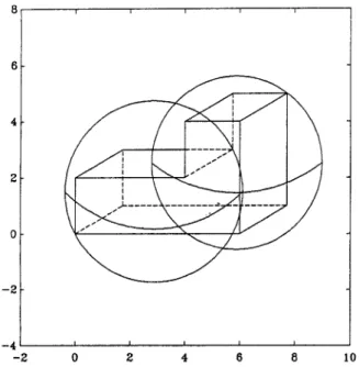
A spherical obstacle was used in the case study in this article. However, arbitrarily shaped or multiple obstacles may be present in an industrial process. To tackle an arbitrarily shaped obstacle utilizing our method, we divide and bound the obstacle by sev- eral spherical obstacles of equal or different radii.

Figure 4 depicts an obstacle bounded by two

spheres. The obstacle resulting from the dividing procedure should be the minimum expansion of the original one. When there are multiple spherical ob- stacles in the workspace, the resulting boundaries will be generated by merging the boundaries corre-

sponding to each obstacle. Taking PWK23 as an ex-

ample, we use two circular OBSZ3 in PWK23 to dem-

ontrate how the boundaries of D1 to D4 are to be

merged. There are three cases to consider: two ob- stacles (a) without intersections, (b) tangential to each other, and (c) overlapping. The merging result for case (a) is shown in Figure 5, and those for cases

(b) and (c) can be obtained similarly.

Obstacle shapes other than a sphere can also be used as the basic element in constructing an irregu- larly shaped obstacle. The choice of which shape to

1.2 1 - 0.8 0.6 0.4 0.2 0 - 6 6 4 2 0 -2 -4 - - - - - -2 0 2 4 6 8 10

Figure 4. Irregularly-shaped obstacles represented by several spheres.

-o.2

t

-0.4 I I I I

-0.5 0 0.5 1 1.5

Figure 5. PWK23 with two obstacles.

use involves a trade-off between a better representa- tion for geometrical analysis and a better element for constructing the target obstacles. For instance, un- like a spherical obstacle, when a donut-shaped ob- stacle is placed with its circular side perpendicular to the ( x l ,

yl)

require dealing with an expanded obstacle, as in the

discussion in section 2.1.2. This indicates that a do-

nut-shaped object may be a better representation for use with our method. However, when an irregu- larly shaped obstacle is constructed using several donut-shaped obstacles with certain orientations, many of the feasible regions may be discarded as a result. The choice of the basic element aforemen- tioned will depend on the shapes of the obstacles encountered during various tasks.

4. PATH PLANNING AND MODIFICATION

Through the above analyses of PWK and OWK, geo-

metric information about a planned path and the

workspaces can be derived for use in modifying in-

feasible portions of the planned path in the work- space. When no obstacle is involved, feasible paths

can always be found between two feasible points

due to the continuity of the workspace. This state- ment is no longer true, however, when certain con- straints due to task requirements and obstacles are imposed. Therefore, the freedom available for modi- fication will depend on task requirements, and ap-

propriate modification strategies will vary accord-

i n g l ~ . ~ With the derived geometrical information

and appropriate modification strategies, the path planning scheme described in the introduction can be utilized to design a kinematically feasible path in the presence of obstacles based on task require- ments. The algorithm for this scheme is as follows: Path Planning Algorithm: Plan a feasible path satis- fying task-level, geometrical, and kinematic con- straints.

Step 1: Design a path by specifying both posi- tion and orientation for each point on the path.

Step 2: Analyze the robot workspace using the

proposed geometrical approach and construct sub- workspaces corresponding to kinematic constraints, such as feasible regions, areas of different configura- tions, and singular areas.

Step 3: Formulate obstacles inside the work-

space constructed in step 2.

Step 4: Derive geometrical information about

the planned path and the robot workspace de- scribed in step 3. Then apply appropriate modifica- tion strategies based on task requirements to modify the infeasible portions of the planned path.

4.1. Path Modification

To accomplish the modification part of step 4 of the path planning algorithm, we need appropriate mod- ification strategies for cases where obstacles are present. For tasks with the position (orientation) limitation, the dof in the orientation (position) can

be utilized for modifi~ation.~ If there are no con-

straints for the given task, then the dof in both posi- tion and orientation can be used for modification. This situation can be taken to be an obstacle avoid- ance problem in the workspace by treating both ob- stacles and infeasible regions due to kinematic con- straints as obstacles. In cases where both position and orientation specifications have to be satisfied, only feasibility can be checked, because there are no dof for modification. We will attempt, then, to de- velop algorithms for modifying an infeasible path in the presence of obstacles by utilizing the dof in posi- tion and orientation, respectively.

4.1 ,I. Position Modification in the Presence of Obstacles

Position modification is intended for cases with the orientation limitation; thus we will use the dof in

position for modification. In general, the length of the end-effector is small compared with the links corresponding to the major joints. The proposed scheme for position modification will enlarge the radius of the obstacle by the length of the end-effec- tor. Hence OWK" will not be affected by the obsta- cle. Because the joint ranges for the minor joints of most industrial robots are quite large, OWK" is usu- ally kinematically feasible. For instance, the PUMA 560 has a range of 280" for joint four, 200" for joint five, and 532" for joint six. However, to avoid hitting itself, joint five cannot have a range greater than 360". This limitation generates infeasible regions in-

side the joint five workspace (OWK5). The infeasibil-

ity in OW& can be resolved by adjusting 81, 82

+

and &.I1 The workspaces of joints four and six are

feasible when their ranges are larger than

With a broad feasible range for 0WKrn, the proposed

scheme will first modify the traces in PWK to obtain

a feasible collision-free wrist path when possible.

Then, based on the new R, and the specified R, on

the planned path, new traces in OWK"' can be de-

rived and modified if necessary. Consequently, the planned path in Cartesian space can be obtained using these new traces. The algorithm is as follows: Collision-Free Position Modification Algorithm: Maintain the orientation specification by modifying the positions in the presence of obstacles.

Ste 1: Enlarge the radius of OBS by the length

Step 2: Find the wrist position

p.,

Derive the corresponding trace of

pu,

noted by trl.

Step 3: Obtain OBSl. Identify the portions of trl in PWKl within the CFR and CPR. For the portion

within the CFR, do the processing in PWK23 without

considering OBS; otherwise, OBS needs to be taken into account.

Step 4: Obtain OBS23. Derive the corresponding

trace of

pw

the infeasible portion of trZ3 to be within feasible

regions when possible. The modified trace is de-

noted by W 2 3 . Possible modifications can be to

move the infeasible portion to be along the bound- ary of feasible regions or just to connect the starting and end locations of the infeasible portion with an arbitrary feasible trace. If modification fails, declare that there is no feasible path available and exit. Note that due to the modification of t ~ 2 3 to '*tr23, trl will

deviate to a new trace Vrl, while trl and 'Yrl may

correspond to the same set of joint variables.

Wu and Young: Path Planning 71 1

Step 5: Find the new wrist orientation " R , corre-

sponding to and '1tr23. Derive the new traces tr"

in OWK"' using "Re derived from "R, and R, on the

initial planned path. Check the feasibility of the trace in OWK, and modify it when infeasible and

possible. If modification fails, declare that there is

no feasible path available and exit.

Step 6: Find the corresponding path in Carte-

sian space using these five newly derived traces.

4.1.2. Orientation Modification in the Presence of Obstacles

In contrast to position modification, orientation modification is developed for cases with the posi- tion limitation. With the position limitation, we need to design the tip path to be collision-free in

step 1 of the path planning algorithm. The dof in

orientation will then be used to modify the traces in the workspaces by maintaining the tip path. Unlike position modification, in orientation modification it is not uncommon for modification to be impossible. With a collision-free tip path, the necessary and suf- ficient condition for a successful modification is that every point on the path must correspond to at least one feasible wrist position and have feasible orienta-

tion(s) in OWK,I2 and all points on the tool need to

be collision-free. Because the tool-tip position is fixed, the feasible wrist positions will be on the sur- face of a sphere that is centered at the tool-tip with the length of the tool as the radius. Thus, to obtain feasible wrist positions, the sphere must intersect

PWK. In addition, at least one of the intersecting

points has to be feasible in PWK and correspond to

feasible orientation(s) in OWK that allows the desig- nated tip location to be reached.

To ensure that points on the tool are collision- free, not only must the wrist be moved away from the obstacle, but also a certain margin must be main- tained between the wrist and the obstacle to keep all the points on the tool collision-free. Because two lengths with different orientations are incorporated into the tool, two dof provide the fixed tip and wrist locations to be connected by these two lengths with various combinations of orientations. To avoid checking for all points on these two lengths with different orientations, we propose to enlarge the ra- dius of the obstacle, as in position modification, in the process of determining the margin kept between the wrist and the obstacle. The enlarged radius, however, will depend on the distance between the obstacle and the tool-tip, and it will be a portion of the tool length instead of the entire length. The rea-

son that the enlarged radius need not be the entire tool length is because the distance between the tool- tip and the obstacle is known in Orientation modifi- cation; consequently, their geometrical relationship can be analyzed and utilized. Thus less feasible re- gions are discarded in orientation modification, which now must satisfy more strict constraints than those for position modification. The enlarged radius

is defined as follows:

Definition 1. Enlarged Radius

(ER):

tool-tip position, the ER is the minimum distance

between the center of the obstacle and the wrist such that all the points on the tool will be collision-

free, no matter what orientations the two lengths of

the tool have.

To modify an infeasible modifiable path, we first find a "most infeasible point" (MIP) for the

points within the infeasible portion of the planned

path." The MIP is then modified into feasible re-

gions with the position of the MIP maintained by

varying its orientation. Among the feasible points

with the same position as MIP, a "most feasible

point" (MFP) is selected to be the modified MIP.

The MIP and MFP are defined as follows":

Definition 2. Most Infeasible Point (MIP):

Among those points within the infeasible portion of

the planned path, MIP is the point that moves the

greatest distance when it is moved into the nearest feasible collision-free location.

Definition 3. Most Feasible Point (MFP):

Among those feasible points with the same position as MIP, MFP is the point that moves the greatest

distance when it is moved to the nearest infeasible location due to kinematic constraints and obstacles. The path will now be replanned by interpolat- ing the orientational parts of the starting point, the

MFP, and the end point of the infeasible portion. If

infeasible portions are still present after replanning, they will be identified and the procedure repeated until a feasible path is found. Because the derivation of MIP and MFP implies that a "most infeasible"

point is modified to a "most feasible" location, the replanning tends to reduce much of the infeasible portion. Consequently, the number of modifica- tions may decrease. The algorithm for orientation modification is as follows.

Yo Collision-Free Orientation Modification Algo-

rithm: Maintain the position specification by modi- fying the orientations in the presence of obstacles.

200°), respectively. The obstacle was defined to be of radius 0.08 m.

Step 1: For each point on the path, find the en-

Iarged radius EX for OBS according to the distance

between the tool-tip and the center of OBS.

Step 2: Using the enlarged obstacle with ER, rotate the tool around the tool-tip to check if each

point on the path has intersecting points with PWK

where the tool is collision-free. If the result is nega- tive, then declare infeasible inputs and exit.

Step 3: For each point, check if at least one of the intersecting points derived in step 2 is feasible in PWK and corresponds to feasible orientation(s) in OWK that allows the designated tip location to be reached. The checking process is divided into sepa-

rate procedures for the CFX and CPR, similar to

those described in the previous section for position modification. However, the checking process here deals with the obstacle of the original radius, be- cause the checking for a collision-free tool has been

performed. If the result is negative, then declare

infeasible inputs and exit.

Step 4: Identify the infeasible portion of the

planned path. Then find the M I P and its corre-

sponding MFP.

Step 5: Replan the path by interpolating the ori-

entational parts of the starting point, the MFP, and

the end point of the infeasible portion.

Step 6: If the replanned portion is feasible, de-

-1.5

0 0.5 1 1.5

-1.5 -1 -0.5 (4

Figure 6. Traces in the positional workspace. (a) Joint one workspace.

maintain the fixed orientation by adjusting the posi- tions on the line. The obstacle was assumed to be

centered at (-0.5, 0.5, 1.5). Based on the discus-

sions in section 2, the initial path was mapped into

PWK and OWK; the traces corresponding to this

path are shown as dotted lines in Figures 6 and 7. Following the collision-free position modification al- gorithm given in the previous section, we enlarged Clare the modification successful and exit. Other-

wise, go back to step 4.

Wu and Young: Path Planning 713

,

Figure 7. Traces in the orientational workspace. (a) Joint

four workspace.

the radius of the obstacle to 0.15 m. In Figure 6a, the

trace, which is the mapping of the designed path on

PWKl, falls within both CFR and CPR. The portion

of the trace that falls within the CPR in PWKl and its

corresponding mapping in PWKZ3 are shown be-

tween two asterisks (*). Therefore, the portion be-

tween the two asterisks had to be modified in the

presence of OBS23 and the rest of the trade did not.

Modifications corresponding to these two regions

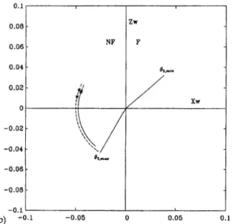
0.08 - 0.06 - 0.04 - NF -0.06 -0.08 -0.1 ~-

-

Figure 7. Traces in the orientational workspace. (b) Joint five workspace.

-.-

( c ) -0.1 -0.05 0 0.05 0.1

Figure 7. Traces in the orientational workspace. (c) Joint

six workspace.

are shown in Figures 8(b) and 9(b). New traces in

PWKl due to the modifications shown in Figures

8(b) and 9(b) are shown in Figures 8(a) and 9(a). The

resulting modified traces in PWKl and PWK23 are

shown as solid lines in Figures 6(a) and 6(b), respec- tively. In Figures 6-9, the modified traces corre-

sponding to the CFR are those between two plus

signs (+). Then, by utilizing the new wrist coordi-

nates obtained from the modified traces in PWK

along with the specified orientation of the initial

path, we obtained new traces in OWK"; they are

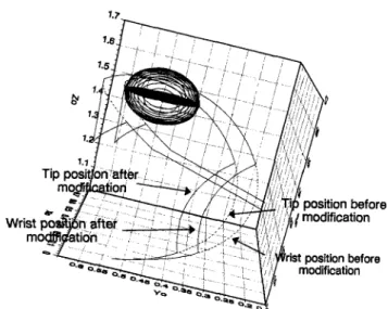
shown as solid lines in Figures 7(a)-(c). These traces were feasible and did not need modification. The resulting modified tip and wrist paths are shown in

Figure 10, where they overlay the original paths.

The scheme successfully modified the original infea- sible line into a feasible one while maintaining the original orientation.

We performed a second simulation to plan a path satisfying a position specification. First, we de- signed an initial path that allowed the robot's tool-

tip to follow a collision-free straight line from (0.87,

0.06, 1.31) to (0.42, 0.21, 1.53) with a fixed orienta-

tion. The obstacle was assumed to be centered at (0.68, 0.24, 1.46). The planned path was found to be infeasible and modifiable. Modification was then performed to maintain the specified positions by ad- justing the orientation on the line. The original and modified tip and wrist paths are shown in Figure 11. The modification scheme maintained the original straight-line path while modifying its orientation.

-1 -0.5 0 0.5 1 1.5

(a) -1.5

Figure 8. Modification for CFR in the positional work- space. (a) Joint one workspace.

Consequently, the original straight-line wrist path was modified to be a curved one.

6. DISCUSSION AND CONCLUSION

Our path planning scheme efficiently designs a kinematically feasible path in the presence of obsta-

- 1 51 &." I

-0.5 0 0.5 1 1.5

(b)-1.5

Figure 8. Modification for CFR in the positional work- space. (b) Joints two and three workspace.

Is------ --1.5 I I ' 0 -1.5 -1 -0.5 0 0.5 1 1.5 (a) Figure 9.

space. (a) Joint one workspace.

Modification for CPR in the positional work-

cles based on task requirements and can be ex- tended to general wrist-partitioned types of robot manipulators and arbitrarily shaped obstacles. In

addition, a merit of the proposed path planning

scheme is that task requirements are incorporated into the planning, which is not well explored in pre-

vious works. A quantitative analysis on the issue of

1.5 1 0 . 5 0 -0.5 -1

1

Figure 9. Modification for CPR in the positional work- space. (b) Joints two and three workspace.

Wu and Young: Path Planning 715

1.7

Wrist

m

plicated obstacle formulation in the robot work- space, the search for feasible paths is time consum- ing. Thus, in a sense, with the proposed obstacle formulation the efficiency in obstacle description and path planning improves at the expense of losing feasible regions in the process of approximation. In addition, we utilize modification strategies to assist in this task-dependent path planning, which in- volves a smaller local search space, and conse- quently demands less running time.

It can be seen that when an irregularly shaped obstacle is represented by several spheres, some of the feasible regions will be discarded in the approxi- mation. It is even more noticeable for those shapes that may not be suitable to be approximated by spheres as the basic element, e.g., a long rod. One resolution will be a trade-off between losing more feasible regions and spending more computation time in using more spheres for approximation. An-

Figure 10, Tip and wrist paths before and after position modification.

efficiency is not discussed in this article, such as complexity analysis or running time comparison with other approaches. Nevertheless, from the qual- itative point of view, the proposed scheme promises to be efficient in both obstacle formulation and path planning. In obstacle formulation, an arbitrarily shaped obstacle is approximated by several spheri- cal obstacles of equal or different radii. Thus simple and similar geometrical analysis can be imposed upon the same shape of obstacles of different sizes. For comparison, a close approximation of the obsta- cle can be achieved at the expense of computation time by applying the cell decomposition approach, or tree-based technique, e t ~ . ~ , ' ~ In turn, with com-

Wrist position

after modification

_...-

other resolution as mentioned in section 3.2 may be that obstacle shapes other than a sphere be used as the basic element in constructing various shapes of obstacles. The choice of which shape to use involves

another trade-off between a better representation

for geometrical analysis and a better element for constructing the target obstacles.

One of our future objectives is to resolve this difficulty by finding more appropriate geometrical representations for obstacles of various shapes. In other words, the representation should be time-effi- cient and result in losing less feasible region. One possible proposal is to perform obstacle formulation

according to the structure of the given robot and

geometrical properties of the link^.^,^^ In some

sense, obstacle formulation will be tackled on the basis of joints; in contrast, in this article the obstacle formulation is in Cartesian space. Note that certain feasible regions cannot be well utilized due to the structure of the links, e.g., the feasible regions in the zig-zag edges of an obstacle. Therefore, obstacle formulation according to the structure and move-

ments of the links may lead to losing less utilizable

feasible regions in the approximation and deserves further exploration.

This work was supported in part by the National Sci- ence Council, Taiwan, R.O.C., under grant NSC 81- 0422-E-009-09.

REFERENCES

figure 11. Tip and wrist paths before and after orienta-

tion modification.

1. E. G. Gilbert and D. W. Johnson, "Distance functions and their application to robot path planning in the

3. 4.

5.

6.

7.

presence of obstacles,” IEEE J. Rob. Autom., 1(1), 21- 30, 1985.

2. J. M. Hollerbach, “Dynamic scaling of manipulator

8. V. Lumelsky, ”Effect of kinematics on motion plan- ning for planar robot arms moving amidst unknown obstacles,” IEEE J. Rob. Autom. 3(3), 207-223, 1987.

modification,” J. Rob. Syst., 9(5), 613-633, 1992. 10. F. L. Litvin, Z. Yi, V. P. Castelli, and C. lnnocenti, trajectories,‘’

wn.

_c.

_wu,

R. P. Paul, “Manipulator Cartesian path control,” IE E E Trans. Sust. Man Cubern., 9(11), 702-711. 1979.

I \ ,I

R. H. Taylor, :‘Planning>nd execution of straight line manipulator trajectories,” IBM 1. Res. Dev., 23(4),

T. Lozano-Perez, “A simple motion-planning algo- rithm for general robot manipulators,” IEEE J. Rob. Autom., 3(3), 224-238, 1987.

K. K. Gupta, “Fast collision avoidance for manipula- tor arms: A sequential search strategy,” I E E E Trans. Rob. Autom., 6(5), 522-532, 1990.

C. S. G. Lee and M. Ziegler, “A geometric approach in solving the inverse kinematics of PUMA robots,”

I E E E Trans. Aerosp. Electron. Syst., 20(6), 695-706, 1984.

424-436, 1979.

”Singularities, configurations, and displacement functions for manipulators,” Int.

1,

11. K. C. Shao and K. Y. Young, ”Path feasibility and modification based on the PUMA 560 workspace analysis,”

1.

12. C. C. Jou, ”On the orientational feasibility of robot manipulators,” Int. Conf. Automation, Robotics, and Computer Vision, 1990, pp. 524-528.

13. J.-C.’ Latombe, Robot Motion Planning, Kluwer Aca- demic Publishers, New York, 1991.