On the Diagnosability of Some Networks by the Comparison Approach

全文

(1)On the Diagnosability of Some Networks by the Comparison Approach ∗ Pao-Lien Lai, Jimmy J. M. Tan † Department of Computer and Information Science National Chiao Tung University Hsinchu, Taiwan 300, R.O.C. Chang-Hsiung Tsai Department of Computer Science and Information Engineering Dahan Institute of Technology Hualien, Taiwan 971, R.O.C. Lih-Hsing Hsu Department of Computer and Information Science National Chiao Tung University Hsinchu, Taiwan 300, R.O.C.. Abstract The classical problem of diagnosability is discussed widely and the diagnosability of many well known networks have been explored. In this paper, we consider the diagnosability of a family of networks, called the Matching Composition Network (MCN); two components are connected by a perfect matching. The diagnosability of MCN under the comparison model is showed to be one larger than that of the component, provided some connectivity constraint. Applying our result, the diagnosability of Hypercubes Qn , Crossed cube CQn , Twisted cube T Qn , and Möbius cube M Qn can all be proved to be n, for n ≥ 4. In particular, we show that the diagnosability of the 4-dimensional hypercube, Q4 , is 4 which is not previously known. ∗ This work was supported in part by the National Science Council of the Republic of China under Contract NSC 90-2213-E-009-149. † Correspondence author: Professor Jimmy J. M. Tan, Department of Computer and Information Science, National Chiao Tung University, Hsinchu, Taiwan 300, R.O.C. e-mail:[email protected].. 1.

(2) Keywords: diagnosability, t-diagnosable, comparison model, Matching Composition Network, MM* model.. 1. Introduction. With the rapid development of technology, the need for high-speed parallel processing systems has continued increasing. The reliability of the processors in parallel computing systems is therefore becoming an important issue. In order to maintain the reliability of a system, whenever a process (node) is found faulty it should be replaced by a fault-free processor (node). The process of identifying all the faulty nodes is called the diagnosis of the system. The maximum number of faulty nodes that the system can guarantee to identify is called the diagnosability of the system. In this paper, we consider the diagnosability of the system under the comparison model, proposed by Malek and Maeng [4, 5]. The diagnosability of some well-known interconnection networks under the comparison model has been investigated. For example, Wang [11] showed that the diagnosability of an n-dimensional hypercube Qn is n for n ≥ 5, and the diagnosability of an n-dimensional enhanced hypercube is n + 1 for n ≥ 6. Fan [3] proved that the diagnosability of an n-dimensional crossed cube is n for n ≥ 4. We study the diagnosability of a family of interconnection networks, called the matching composition networks (MCN), which can be recursively constructed. MCN includes many well-known interconnection networks as special cases, such as Hypercubes Qn , Crossed cubes CQn , Twisted cubes T Qn and Möbius cubes M Qn . Basically, MCN and these mentioned cubes are all constructed from two graphs G1 and G2 with the same number of nodes, by adding a perfect matching between the nodes of G1 and G2 . We shall call these two graphs G1 and G2 as the components of MCN. Our main result is the following. Suppose that the number of nodes in each component is. 2.

(3) at least t + 2, the order (which will be defined subsequently) of each node in Gi is t, and the connectivity of Gi is also t, i = 1, 2. We prove that the diagnosability of MCN constructed from G1 and G2 is t + 1, for t ≥ 2. In other words, the diagnosability of MCN is increased by 1 as compared with those of the components. Using our result, it is straightforward to see that the diagnosability of Hypercube Qn , Crossed Cube CQn , Twisted Cube T Qn and Möbius cube M Qn are n for n ≥ 4. Some of these particular applications are all previously known results [3, 11], using rather lengthy proofs. Our approach unifies these special cases and our proof is much simpler. We would like to point out that the diagnosability of the 4-dimensional Hypercube Q4 is 4, which is not previous resolved [11]. The paper is organized as follows:Section 2 introduces the comparison model for diagnosis. Section 3 provides preliminaries. In Section 4, we present the Matching Composition Network and discuss its diagnosability. In Section 5, we propose that hypercube Q4 is 4-diagnosable. Finally, our concluding remarks are offered in Section 6.. 2. The Comparison Model for Diagnosis. For the purpose of self-diagnosis of a given system, several different models have been proposed in literature [1, 4, 5, 6, 7, 9, 10]. Preparata, Metze and Chien [6] first introduced a model, so called PMC-model, for system level diagnosis in multiprocessor systems. In this model, it is assumed that a processor can test the faulty or fault-free status of another processor. The comparison model, called MM model, proposed by Maeng and Malek [4, 5], is considered to be another practical approach for fault diagnosis in multiprocessor systems. In this approach, the diagnosis is carried out by sending the same testing task to a pair {u, v} of processors and comparing their responses. The comparison is performed by a third processor w that has directed communication link to both processors u and v. The third processor w is called a comparator of u and v. 3.

(4) If the comparator is fault-free, a disagreement between the two responses is an indication of the existence of a faulty processor. To gain as much knowledge as possible about the faulty status of the system, it was assumed that a comparison is performed by each processor for each pair of distinct neighbors with which it can communicate directly. This special case of MM-model is referred to as the MM*-model. Sengupta and Dahbura [8] studied the MM-model and the MM*-model, gave a characterization of diagnosable systems under the comparison approach, and proposed a polynomial time algorithm to determine faulty processors under MM*-model. In this paper, we study the diagnosability of M CN (which will be defined subsequently) under MM*-model. In the study of multiprocessor systems, the topology of networks is usually represented by a graph G = (V, E), where each node v ∈ V represents a processor and each edge (u, v) ∈ E represents a communication link. The diagnosis by comparison approach can be modeled by a labeled multigraph, called comparison graph, M = (V, C), where V is the set of all processors and C is the set of labeled edge. A labeled edge (u, v)w ∈ C, with w being a label on the edge, connects u and v, which implies that processors u and v are being compared by w. Under the MM-model, processor w is a comparator for processor u and v only if (w, u) ∈ E and (w, v) ∈ E. The MM*-model is a special case of the MM model, it is assumed that each processor w such that (w, u) ∈ E and (w, v) ∈ E is a comparator for the pair of processors u and v. Obviously, comparison graph M = (V, C) can be a multigraph, for the same pair of nodes may be compared by several different comparators. For (u, v)w ∈ C, the output of comparator w of u and v is denoted by r((u, v)w ), a disagreement of the outputs is denoted by the comparison results r((u, v)w ) = 1, whereas an agreement is denoted by r((u, v)w ) = 0. In this paper, we have the following assumptions: (1) All faults are permanent; (2) a faulty processor produces incorrect outputs for each of its given testing tasks; (3) the output. 4.

(5) of a comparison performed by a faulty processor is unreliable; and (4) two faulty processors with the same input do not produce the same output. Therefore, if the comparator w is fault-free and r((u, v)w ) = 0, then u and v are both fault-free. If r((u, v)w ) = 1, then at least one of u, v and w must be faulty. The set of all comparison results of a multicomputer system that are analyzed together to determine the faulty processors is called a syndrome of the system. For a given syndrome σ, a subset of nodes F ⊆ V is said to be consistent with σ, if syndrome σ can be produced from the situation that all nodes in F are faulty and all nodes in V − F are fault-free. Because a faulty comparator can lead to unreliable result, a given set F of faulty nodes may produce various syndromes. Let σ ∗ (F ) = {σ|σ is a syndrome which can be produced from the situation that all nodes in F is faulty and all nodes in V − F is fault-free}. Two distinct sets S1 , S2 ⊂ V are said to be indistinguishable if and only if σ ∗ (S1 ). T. σ ∗ (S2 ) 6=. Ø; otherwise, S1 , S2 are said to be distinguishable. And, a system is said to be t-diagnosable if for every syndrome, there is a unique set of faulty nodes that could produce the syndrome, provided the number of faulty nodes does not exceed t.. 3. Preliminaries. We need some definitions and previous results for further discussion. Let G be a graph with V (G) represent the node set of G and E(G) the edge set of G. Assume U ⊆ V (G). G[U ] denote the subgraph of G induced by the node subset U of G and U = V (G) − U . The vertex connectivity (simply abbreviated as connectivity) of a network G = (V, E), denoted by κ(G) or κ, is the minimum number of vertices whose removal leaves the remaining graph disconnected or trivial. Assume that V1 , V2 are two disjoint nonempty subsets of V (G). The neighborhood set of V1 in V2 , N (V2 , V1 ), is defined as {x ∈ V2 | there exists a node y ∈ V1 5.

(6) such that (x, y) ∈ E(G)}. A vertex cover of G is a subset K ⊆ V (G) such that every edge of E(G) has at least one end vertex in K. A vertex cover set with the minimum cardinality is called the minimum vertex cover. Given a graph G, let M be the comparison graph of G. For a node v ∈ V (G), we set S. Xv to be the set {u | (v, u) ∈ E(G)} {u | (v, u)w ∈ E(M ) for some w} and Yv to be the set {(u, w) | u, w ∈ Xv and (v, u)w ∈ E(M )}. In [8], the order graph of node v, is defined as Gv = (Xv , Yv ) and the order of the node v, denote by orderG (v), is defined as the cardinality of a minimum vertex cover of Gv . Let U ⊂ V (G). We use T (G, U ) to denote the set {u | (v, u)w ∈ E(M ) and w, v ∈ U, u ∈ U }. We observe that T (G, U ) = N (U , U ) if G[U ] is connected for U ⊂ V (G) and |U | > 1. This observation can be extended to the following lemma. Lemma 1 Let U be a subset of V (G) and G[Ui ], 1 ≤ i ≤ k, be the connected components of G[U ] such that U =. k [. Ui . Then T (G, U ) =. i=1. k [. {U , Ui ) | |Ui | > 1}.. i=1. 0. 3 4. 7. 5. 6. 1. 2. Figure 1: Example for T (G, U ) of Q3 . In Fig. 1, taking Q3 as an example, we have T (G, U ) = {4, 5, 6, 7}, where U = {0, 1, 2, 3}. The next lemma follows directly from the definition of connectivity of G. Lemma 2 [2] Let G be a connected graph and U be a subset of V (G). Then |N (U , U )| ≥ κ(G) if |U | ≥ κ(G), and |N (U , U )| = |U | if |U | < κ(G). 6.

(7) There are several different ways to verify a system to be t-diagnosable under the comparison approach. In this paper, we need three theorems given by Sengupta and Dahbura [8]. The first two are necessary and sufficient conditions for ensuring distinguishability, the third one is a sufficient condition for verifying a system to be t-diagnosable. Theorem 1 [8] For any two distinct subsets S1 ,S2 of V (G) is a distinguishable pair if and only if at least one of the following conditions is satisfied: (See Fig. 2) S. (i) ∃i, k ∈ V − S1 − S2 and ∃j ∈ (S1 − S2 ) (S2 − S1 ) such that (i, j)k ∈ C, (ii) ∃i, j ∈ S1 − S2 and ∃k ∈ V − S1 − S2 such that (i, j)k ∈ C, or (iii) ∃i, j ∈ S2 − S1 and ∃k ∈ V − S1 − S2 such that (i, j)k ∈ C.. S2. S1. (i). (i) (ii). (iii). V. Figure 2: Description for distinguishability.. Theorem 2 [8] A system G is t-diagnosable if and only if (1) orderG (v) ≥ t for any node v in G and (2) at least one of the conditions of Theorem 1 is satisfied for each distinct pair of sets S1 , S2 ⊂ V such that |S1 | = |S2 | = t. Theorem 3 [8] A system G with N nodes is t-diagnosable if (1) N ≥ 2t + 1; (2) orderG (v) ≥ t for any node v in G; 7.

(8) (3) |T (G, U )| > p for each U ⊂ V (G) such that |U | = N − 2t + p and 0 ≤ p ≤ t − 1. According to the above three theorems, we observe that condition (3) of Theorem 3 restricts G satisfying the first condition of Theorem 1 and ignores conditions 2 and 3. Hence, we present a hybrid theorem to test whether a system is t-diagnosable. Theorem 4 A system G with N nodes is t-diagnosable if and only if (1) N ≥ 2t + 1; (2) orderG (v) ≥ t for any node v in G; (3) for any two distinct subsets S1 , S2 ⊂ V (G) such that |S1 | = t and |S2 | = t either (a) |T (G, U )| > p, where U = V (G) − (S1. S. S2 ), and |S1. T. S2 | = p. or (b) S1 and S2 satisfy condition (ii) or (iii) of Theorem 1. Proof: Conditions (1) and (2) are same as conditions (1) and (2) of Theorem 3, and condition (3) includes condition (3) of Theorem 3 and all cases of Theorem 1. Consider condition (3.a). S1 and S2 are distinct subsets of V (G) with |S1 | = |S2 | = t, U = V (G) − (S1. S. S2 ), and |S1. T. S2 | = p. Then 0 ≤ p ≤ t − 1 and |U | = N − 2t + p. If |T (G, U )| > p,. it implies that S1 and S2 satisfy condition (i) of Theorem 1. Combining condition (3.a) and (3.b), by Theorems 1 and 2, this theorem follows.. 4. 2. Diagnosability of Matching Composition Networks. Now, We define the Matching Composition Network(MCN) as follows. Let G1 and G2 be two graphs with the same number of nodes. Let L be an arbitrary perfect matching between the nodes of G1 and G2 ; i.e., L is a set of edges connecting the nodes of G1 and G2 in a one to one fashion, the resulting composition graph is called a Matching Composition Network (MCN). For convenience, G1 and G2 are called components of the MCN. Formally, we use 8.

(9) the notation G(G1 , G2 ; L) (simply abbreviated as G1L2 ) to denote a MCN, which has node set V (G(G1 , G2 ; L)) = V (G1 ). S. V (G2 ) and edge set E(G(G1 , G2 ; L)) = E(G1 ) ∪ E(G2 ) ∪ L.. See Fig. 3. What we have in mind is the following: Let G1 and G2 be two t-connected networks with the same number of nodes and orderGi (v) ≥ t for any node v in Gi ,where i = 1, 2, and let L be an arbitrary perfect matching between the nodes of G1 and G2 . Then the degree of any node v in G(G1 , G2 ; L) as compared with that of node v in Gi for i = 1, 2, is increased by 1. We expect that diagnosability of G(G1 , G2 ; L) is also increased to t + 1. For example, Hypercube Qn+1 is constructed from two copies of Qn adding a perfect matching between the two and the diagnosability is increased from n to n + 1 for n ≥ 5. Other examples such as Twisted cube T Qn+1 , Crossed cube CQn+1 , Möbius cube M Qn+1 are all constructed recursively using the same method as above.. v. v'. G1. v". G2. Figure 3: Description of orderG1L2 (v).. Theorem 5 Let G1 and G2 be two networks with the same number of nodes, and t be a positive integer. Suppose that orderGi (v) ≥ t for any node v in Gi , where i = 1, 2. Then orderG1L2 (v) ≥ t + 1 for node v in G(G1 , G2 ; L). Proof: See Fig. 3. Let v be a node of G(G1 , G2 ; L). Without loss of generality, we 0. 0. 0. assume that v ∈ V (G1 ), v ∈ V (G2 ) and (v, v ) ∈ L. Of course, node v is connected to 9.

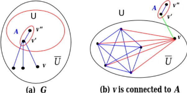
(10) 00. at least one node v in V (G2 ). Let G(v, G1 ) and G(v, G(G1 , G2 ; L)) be the order graph of v in graph G1 and G(G1 , G2 ; L), respectively. We observe that G(v, G1 ) is a proper 0. 00. subgraph of G(G1 , G2 ; L), both v and v are in the latter, none of them in the former, 0. 00. and (v , v ) is an edge in G(G1 , G2 ; L). Therefore, every vertex cover of the order graph G(v, G(G1 , G2 ; L) contains a vertex cover of the order graph G(v, G1 ). Besides, any vertex 0. 00. cover of G(v, G(G1 , G2 ; L)) has to include at least one of v and v . Thus, orderG1L2 (v) ≥ orderGi (v) + 1 for any node v in G1L2 and Gi , where i = 1, 2, repectively. This completes the proof.. 2. We need the following lemma later in Theorem 6. Lemma 3 [3] Let G be a t-connected network, and orderG (v) ≥ t for any node v in G. Suppose that U is a subset of nodes of V (G) with |U | ≤ t. Then |T (G, U )| = |U |. Proof: By assumption |U | ≤ t and κ(G) ≥ t, we prove the lemma by two cases; the first for |U | < κ(G) and the second for |U | = κ(G). If |U | < κ(G), by Lemma 1 and Lemma 2, |T (G, U )| = |N (U , U )| = |U |. This case holds. Now, suppose that |U | = κ(G). We observe that, adding any node v of U to U , the S. induced subgraph G[U {v}] forms a connected graph. It implies that every node v of U is adjacent to every connected components of G[U ]. We claim that the subgraph induced by U contains a connected component A with cardinality at least 2 (See Fig. 4(a)). Then, the connected component A is adjacent to all nodes in U and, so |T (G, U )| ≥ |U |. Now, we prove the claim. Suppose on the contrary that every connected component of the subgraph induced by U is an isolated node. Let v be an arbitrary node in U , and let Gv = (Xv , Yv ) be the order graph of v in G. Then U − {v} is a vertex cover of Gv , because every connected component of G[U ] is an isolated node v. Since |U | ≤ t, we have |U − {v}| ≤ t − 1. Therefore, the cardinality of a minimum vertex cover of the order graph 10.

(11) Gv is at most t − 1. This contradicts to the hypothesis of orderG (v) ≥ t for any node v in G. So G[U ] has a connected component A with cardinality at least 2 (See Fig. 4(b)). This proves the claim, and the lemma follows.. 2. U. U. v". A v'. v". A. v. v'. v. U. U. (b) v is connected to A. (a) G. Figure 4: Example of the T (G, U ) when |U | = t .. We are now ready to state and prove a theorem about the diagnosability of Matching Composition Network under the comparison model. As an illustration, the conditions of the following theorem are applicable to some well-known interconnection networks, such as Q n , CQn , T Qn and M Qn for n = t ≥ 3. Theorem 6 For t ≥ 2, let G1 and G2 be two graphs with the same number of nodes N , where N ≥ t + 2. Suppose that orderGi (v) ≥ t for any node v in Gi and the connectivity κ(Gi ) ≥ t, where i = 1, 2. Then MCN G(G1 , G2 ; L) is (t + 1)-diagnosable. Proof: Since |V (G1 )| = |V (G2 )| = N , 2N ≥ 2(t + 2) > 2(t + 1) + 1. By Theorem 5, orderG1L2 (v) ≥ t + 1 for any node v in G1L2 . It remains to prove that G(G1 , G2 ; L) satisfies condition 3 of Theorem 4. Let S1 and S2 be two distinct subsets of V (G) with the same number t + 1 of nodes , and let |S1. T. S2 | = p, then 0 ≤ p ≤ t. In order to prove this theorem, we will prove that S1. and S2 are distinguishable, i.e., they satisfy either condition (3.a) or (3.b) of Theorem 4.. 11.

(12) Let G = G(G1 , G2 ; L), U = V (G) − (S1 U = U1. S. U2 with Ui = U. T. S. S2 ), then |U | = 2N − 2(t + 1) + p. Let. V (Gi ) and Ui = V (Gi ) − Ui , i = 1, 2. Without loss of generality,. we assume that |U1 | ≥ |U2 |. Let |U1 | = n1 , |U2 | = n2 , n1 + n2 = 2(t + 1) − p, and n1 ≤ n2 . Since 0 ≤ n1 ≤. 2(t+1)−p . 2. The maximum value of n1 is equal to t + 1 when p = 0 and. n2 = t + 1. According to different values of n1 and n2 , we divide the proof into two cases. The first case n2 ≤ t which implies n1 ≤ t. The second case n2 > t, and this case is further divided into three subcases n1 < t, n1 = t and n1 > t. Case 1: n1 ≤ t and n2 ≤ t. By Lemma 3, we have |T (G, U )| ≥ |T (G1 , U1 )| + |T (G2 , U2 )| = |U1 | + |U2 | = n1 + n2 = 2(t + 1) − p. We know that 0 < p ≤ t, |T (G, U )| ≥ 2(t + 1) − p > p and condition (3.a) of Theorem 4 is satisfied. Case 2: n2 > t. We discuss the case as three subcases, (2a)n1 < t, (2b)n1 = t and (2c)n1 > t. Subcase 2a: n1 < t. Since κ(G1 ) ≥ t and |U1 | = n1 < t, G[U1 ] is connected. By lemma 1 and lemma 2, T (G1 , U1 ) = N (U1 , U1 ) = n1 . There are n1 and n2 nodes in U1 and U2 , respectively, and n2 = 2t + 2 − p − n1 (See Fig. 5). If all the nodes in U1 are adjacent to some n1 nodes in U2 , there are still at least n2 − n1 = 2t + 2 − p − 2n1 nodes in U2 such that each of them is adjacent to some node in U1 under the matching L. So, |T (G, U )| ≥ |T (G1 , U1 )|+(n2 −n1 ) = n1 + (n2 − n1 ) = n2 . Because n2 > t ≥ p, the proof of this subcase is complete. Subcase 2b: n1 = t. We know that n1 + n2 = 2(t + 1) − p, 0 ≤ p ≤ t, n2 > t and n1 = t, the only two valid values for n2 are t + 1 and t + 2. n2 = t + 1 implies p = 1, and n2 = t + 2 implies p = 0. By 12.

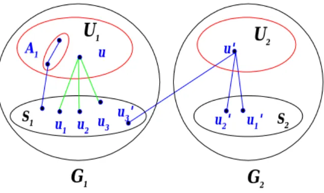
(13) U1. U2. U1. U2. G1. G2. Figure 5: Illustration of Subcase2a. Lemma 3, |T (G1 , U1 )| = |U1 | = t ≥ 2 > p for p = 0 or 1. Then the subcase holds. Subcase 2c: n1 > t. Observing that 0 ≤ n1 ≤. 2(t+1)−p , 2. where 0 < p ≤ t and n2 ≥ n1 > t, so n1 = n2 = t + 1.. It also implies p = 0. Here, we will prove that the subcase satisfies either condition (3a) or condition (3b) of Theorem 4. First, if the subgraph induced by U contains a connected component A1 with cardinality at least 2 (See Fig. 6) and it is adjacent to some node in U . Then |T (G, U )| > 0 = p, and condition (3.a) of Theorem 4 is satisfied. Otherwise, every connected component of U contains a single node only. We know that S1 and S2 are distinguishable if there exists a path hu1 → u → u2 i such that u ∈ U , and u1 , u2 ∈ S1 − S2 or u1 , u2 ∈ S2 − S1 . If p = 0, it implies S1. T. S2 = φ, any node u in G[U ]. with degree more than 2 must be connected to at least two nodes in S1 or S2 (See Fig. 6). By Theorem 5, orderG1L2 (v) ≥ t + 1 for any node v in G1L2 , therefore deg(v) ≥ t + 1 for any node v. Since t ≥ 2, condition (3.b) of Theorem 4 is satisfied. Hence, the subcase holds.. 2. 13.

(14) U1. A1. S1. u1 u2 u3. U2. u'. u. u3'. u2'. G1. u1'. S2. G2. Figure 6: Example of Subcase 2c. Corollary 1 Let G1 and G2 be two graphs with the same number of nodes N . Suppose that both G1 and G2 are t-diagnosable and have connectivity κ(G1 ) = κ(G2 ) ≥ t, where t ≥ 2. Then MCN G(G1 , G2 ; L) is (t + 1)-diagnosable.. 5. Hypercube Q4 is 4 − diagnosable. In [11], D. Wang has proved that the diagnosability of hypercube-structured multiprocessor systems under the comparison model is n when n ≥ 5. However, the diagnosability of Q4 is not known to be 4. We now prove it. We observe that Q3 is 3-connected, orderQ3 (v) = 3 for any node v in Q3 , and the number of nodes of Q3 is 8, 8 ≥ t + 2 = 5 for t = 3. It is well-known that Q4 can be constructed from two copies of Q3 by adding a perfect matching between these two copies. Therefore, by Theorem 6, Q4 is 4-diagnosable. However Q3 is not 3-diagnosable. In Fig. 7, there is a Q3 , let S1 = {0, 5, 7} and S2 = {2, 5, 7}. Then, by Theorem 1, S1 and S2 are not distinguishable as shown in the next figure.. As we observe that most of the related results on diagnosability of multiprocessors systems 14.

(15) 0. 1. 3 4. 7. 5. 6. (a) Q3. 0. 2. 4. S1. 7. 3. 5. S2 2. 1. 6. (b) Q3. Figure 7: S1 = {0, 5, 7} and S2 = {2, 5, 7} are not distinguishable. [3, 11] are based on a sufficient theorem, namely Theorem 3. Not satisfying this sufficient condition, such as hypercube Q4 , it does not necessarily imply that it is not 4-diagnosable. Therefore, we propose a hybrid condition, 3(a) and 3(b) of Theorem 4, to check the diagnosability of multiprocessor systems under the comparison model. It is a necessary and sufficient condition and it is more powerful to use. Applying our Theorem 4 and Theorem 6, we show that the diagnosability of Q4 is indeed 4.. 6. Conclusion. In this paper, we propose a necessary and sufficient theorem to verify the diagnosability of multiprocessor systems under the comparison-based model. The conditions of this theorem include all the cases of the original necessary and sufficient condition stated in Theorem 1. Therefore, it is more suitable for verifying the diagnosability of a system. Then we propose a family of interconnection networks which are recursively constructed, called matching composition networks. Each member G(G1 , G2 ; L) of this family are constructed from a pair G1 and G2 of lower dimensional networks with the same number of nodes, joining by a perfect matching L between the two. Applying Theorem 6 in this paper, we show that the diagnosability of G(G1 , G2 ; L) is one larger than those of the G1 and G2 , provided some regular conditions stated in Theorem 6. 15.

(16) Many well-known interconnection networks, such as the Hypercubes Qn , the Crossed cubes CQn , the Twisted cubes T Qn , and the Möbious cubes M Qn , belong to our proposed family. We note here that these special cases all satisfy the condition of Theorem 6 for n ≥ 4. Thus, their diagnosabilities are n, for n ≥ 4. In particular, the diagnosability of the 4dimensional hypercube Q4 is 4.. References [1] Evangelos Kranakis and Andrzej Pelc, ”Better Adaptive Diagnosis of Hypercubes,” IEEE Trans. on Computers, vol. 49, no. 10, pp. 1013-1020, Oct. 2000. [2] J. Fan, “Diagnosability of Crossed Cubes under the Two Strategies,” Chinese J. Computers, vol. 21, no. 5, pp. 456-462, May 1998. [3] J. Fan, “Diagnosability of Crossed Cubes under the Comparison Diagnosis Model,” manuscript. [4] M. Malek, ”A Comparison Connection Assignment for Diagnosis of Multiprocessor Systems,” Proc. 7th Int’l Symp. Computer Architecture, pp. 31-35, 1980. [5] J. Maeng and M. Malek, “A Comparison Connection Assignment for Self-Diagnosis og Multiprocessors Systems,” Proc. 11th Int’l Symp. Fault-Tolerant Computing, pp.173175,1981. [6] F. P. Preparata, G. Metze, and R. T. Chien, ”On the connection Assignment Problem of Diagnosis Systems,” IEEE Trans. on Electronic Computers, vol. 16, no. 12, pp. 848-854, Dec. 1967. [7] Sasidhar Koppolu and Abhijit Chatterjee, ”Hierarchical Diagnosis of Identical Units in a System,” IEEE Trans. on Computers, vol. 50, no. 2, pp. 186-191, Feb. 2001. [8] A. Sengupta and A. Dahbura, “On Self-Diagnosable Multiprocessor Systems: Diagnosis by the Comparison Approach,” IEEE Trans. on Computers, vol. 41,no 11, pp. 13861396, Nov. 1992. [9] Stefano Chessa and Piero Maestrini, ”Correct and Almost Complete Diagnosis of Processor Grids,” IEEE Trans. on Computers, vol. 50,no 10, pp. 1095-1102, Oct. 2001.. 16.

(17) [10] Toru ARAIK and Yukio SHIBATA, ”Diagnosability of Butterfly Networks under the Comparison Approach,” IEICE Trans. Fundamentals, vol. E85-A, no. 5, pp. 1152-1160, May 2002. [11] D. Wang, “Diagnosability of Hypercubes and Enhanced Hypercubes under the Comparison Diagnosis Model,” IEEE Trans.Computers, vol.48, no.12, pp. 1369-1374, 1999.. 17.

(18)