Application of Cesàro Mean and the L-curve for the Deconvolution Problem

(1)

Please cite this paper as follows:

L.Y. Chen, J.T. Chen, H.-K. Hong and C.H. Chen, Application of Cesàro Mean and the L-curve for

the Deconvolution Problem.

,

Soil Dynamics and Earthquake Engineering, Vol.14, pp.361-373, 1995.

(2)

E L S E V I E R 0 2 6 7 - 7 2 6 1 ( 9 5 ) 0 0 0 0 3 - 8

Soil Dynamics and Earthquake Engineering 14 (1995) 361-373

Application of Ces/kro mean and the L-curve for the

deconvolution problem

L. Y. Chen

Department of Civil Engineering, Kao Yuan Jr. College of Technology and Commerce, Taiwan

J. T. Chen*

Department of Harbor and River Engineering, National Taiwan Ocean University, Keelung, Taiwan

&

H.-K. Hong & C. H. Chen

Department of Civil Engineering, National Taiwan University, Taipei, Taiwan (Received 15 September 1994; accepted 5 December, 1994)

N O T A T I O N an A ( f ) C(k, r) c[,

f

Cn

Hs

I,:;

I';u( t - ~-)

N r

Sn

t rbg(f) Tgb(f) T(t)

In this paper, the Cesfiro mean technique is applied to regularize the divergent problem which occurs in ground motion deconvolution analysis in geotechnical engineering. To deal with this ill-posed problem, we use the corner of the L-curve as the compromise point to determine the optimal order of Cesfiro mean so that the high frequency content can be suppressed instead of engineering judgement using the concept of a cutoff frequency. The fractional order of Ces~ro mean has been derived and used to fulfill this purpose. From the examples shown, it is found that the wave form including maximum acceleration can be accurately predicted and that both the high frequency content and divergent results can be avoided by using the proposed regularization technique.

Key words: Cesfiro mean, L curve, deconvolution

~P(f) the nth term o f series

Amplitude o f transfer function

Cesaro m e a n o p e r a t o r o f order r with k terms binomial coefficient

exciting frequency

nth frequency in the Fourier t r a n s f o r m thickness o f soil layer

complex wave n u m b e r

reproducing kernel (Fejer kernel) total n u m b e r in Fourier transform order o f Cesfiro m e a n

partial sum time

transfer function o f devonvolution transfer function o f convolution

traction on the ground surface in the time d o m a i n * Correspondence to J. T. Chen. u

up(t)

~g(t)

ub(t)

~b(t) Ub(f) Up(f) U ( f )

v~

w;

r(x)

traction on the ground surface in the frequency domain

displacement

displacement o f the ground surface

contaminated displacement o f the ground surface

displacement o f the basement

calculated displacement deconvoluted from ~g (t) Fourier coefficient o f u b

Fourier coefficient o f Ug

Fourier coefficient o f u

shear wave velocity o f the soil layer ith weight o f Cesgtro mean with r order G a m m a function o f x

hysteretic d a m p i n g ratio o f the soil layer

361

1. I N T R O D U C T I O N

Inverse problems are presently becoming m o r e impor- tant in m a n y fields o f science and engineering. The deconvolution p r o b l e m can be seen as one inverse

(3)

contaminated

+--- ground mot/on ground motion

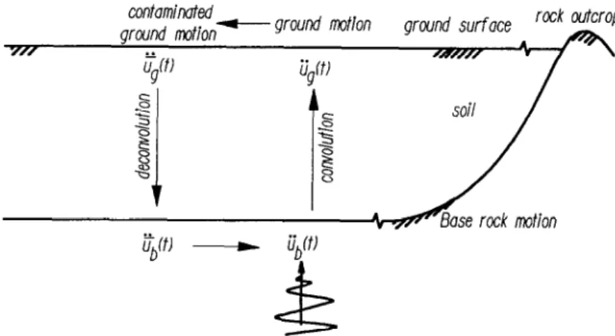
Fig. 1. Single layer soil model.

problem. Sometimes, unreasonable results occur in deconvolution analysis due to the damping mechanism and contaminated errors in the input motion. For example, the SHAKE program7 has too much high frequency response, and in some cases divergent results, in deconvolution analysis as mentioned by Chen.’ Mathematically speaking, the deconvolution problem is ill-posed since the solution is very sensitive to the given data. This phenomenon will become more serious when either the deconvolution depth is deeper or the damping ratio is larger. Although the damping model of soils is not clearly understood, it is always assumed to be hysteretic damping in engineering practice. This paper focuses on a treatment for divergence due to noise. The material properties are assumed to be known, i.e. the source identification is considered instead of system parameter identification. Such a divergent problem could be avoided by using a cutoff frequency in the SHAKE program or using by regularization methods. The former method utilizes a rectangular window to eliminate all the high frequency contents larger than the cutoff frequency. Nevertheless, how to choose a suitable cutoff frequency depends on the engineering judgement in engineering practice. Furthermore, the side lobe of the rectangular window is large. To find an optimum window with a general rule is a key step in solving such problems. The regularization techniques have been successfully

10'

- Convolution ;'

- 10' --- Deconvolution ,’

A ,,,’

applied to circumvent the influence of noise. For example, three regularization techniques have been applied to direct problems by Chen and Hong*-5 when the solution is contaminated with noise. The three methods can effectively suppress noise propagation.

In this paper, we shall employ one of the regularization methods, the Cesaro regularization technique,8 to circumvent the ill-posed problem. In other words, an optimum Cesaro window will be introduced. The Cesdro window can redistribute the amplitude of frequency content in the system kernel; therefore, an ill-posed problem can be transformed into a well-posed one by choosing the appropriate order of the Cesaro mean. The appropriate order is determined according to the compromise between regularization error (due to data smoothing) and perturbation error (due to noise disturbance).’ The corner of the L- curve can provide the compromise point and will be elaborated on later. Finally, two examples, single layer soil with artificial noises and multiple layer soils at the LSST site in Lotung, Taiwan with measured data, will be shown to illustrate the validity of the proposed technique.

2. FORMULATION OF THE DECONVOLUTION PROBLEM

In general, the deconvolution problem can be described

10 Cesaro Order k Y.- 1s s g10 -21 ‘I; E 2 10 -1 2f

10 -'1 Total number n = El192

._

O.'l

Exciting Frequenc:‘(Hz) 160

Fig. 2. Transfer functions of convolution and deconvolution.

10 100 1000 1oc

Number of Terms i

(4)

Application of Ceshro mean and the L-curve for the deconvolution problem

363 14 12 iO 8

Klv(t

-

r)

6

4

2 o

i - 3 - 2 - 1 N=10 ! = 7 i = 6 1 2 3 (t - ~)

for increasing number N.

o f its generality, a h o m o g e n e o u s soil layer underlain by a horizontally extended basement can be used• It is assumed that the soil is linearly elastic with d a m p i n g o f the hysteretic type• F o r a SH wave vertically p r o p a g a t i n g in the soil layer, the frequency domain transfer function between the surface motion and basement m o t i o n in the frequency domain can be derived and represented as

T g b ( f ) _ Ug(f)

Ub(f )

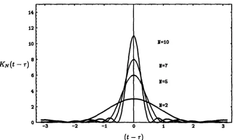
(1)

Fig. 4. The reproducing kernel as shown in Fig. 1, where the b o u n d a r y condition o f traction

T(t)

and displacement

u(t)

in the time domain or 2P(f) and

U ( f )

in the frequency domain are prescribed over the surface o f the ground, but the stress and displacement fields under the ground surface are b o t h unknown.

Conventionally, as used in S H A K E analysis, deconvolution analysis is performed in the frequency domain. We can formulate the associated transfer function to investigate the p r o b l e m of high frequency divergency o f this analysis• As a simple example but without loss

(a) 0.20 Base Motion A m a x --= 0.I00 g | O.lO o "~ - 0 . 0 0 g "~ -0.10 - 0 . 2 0 0 10 20 30 40 Time (see) (b) 0.002 J B a s e M o t i o n ! o 0.001

5

0.000 0 10 20 30 40 Frequency (Hz) 0.20 -_ 0 . 1 0 - O ~ -0.00 - '~ - 0 . 1 0 - 0 . 2 0 0.008 (a) S u r f a c e Motion Amax = 0.162 g Depth = 0 m 10 20 30 40 Time (sec) (b) , ~ 0 . 0 0 6 o 0.004 0.002 0.000 S u r f a c e Motion Depth = 0 m , , , , , , , , i , , , , , , J J , l , l , , , , , , , i , , i , , , , , , 10 20 30 40 Frequency (Hz)

Fig. 5. The original input motion given at the basement level. Fig. 6. Ground surface motion convoluted from the given base- (a) Time history. (b) Fourier coefficient spectrum, ment motion. (a) Time history. (b) Fourier coefficient spectrum.

(5)

0 . 2 0.1 e!

.2

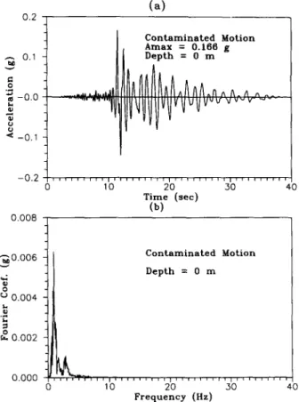
~ - o . o - 0 . 1 - 0 . 2 0 . 0 0 8 (a) C o n t a m i n a t e d M o t i o n A m a x = 0 . 1 6 6 g D e p t h = 0 m 0 10 2 0 30 40 T i m e (see) (b) " ~ 0 . 0 0 6 o 0.004 0.002 0 . 0 0 0 C o n t a m i n a t e d Motion D e p t h = 0 m

I

i i , ~ l j l , l , l l , , , l , l l , , l j , , , l , l , , , l l l , , , 0 I 0 2 0 3 0 4 0 F r e q u e n c y (Hz)

Fig. 7. Contaminated ground surface motion. (a) Time history. (b) Fourier coefficient spectrum.

4 0 0 2 0 0 e., o ~

o.

ID -200 (a) C e s a r o Order = 0 A m a x = 3 4 6 . 4 4 g D e p t h = 50 m -400 0 1 0 2 0 3 0 4 0 T i m e ( s e e ) ( b ) 0 . 0 0 2 Cesaro Order = 0 Depth = 50 m o ~ 0 . 0 0 1 0 . 0 0 0 0 10 2 0 30 4 0 F r e q u e n c y (Hz)

Fig. 8. Basement motion without using rcgularization decon- voluted from the contaminated ground surface motion. (a)

Time history. (b) Fourier coefficient spectrum.

~'~ 1 0 0

; ~ L - c u r v e for D e p t h 0 - 50 m

Order at the corner = 4 . ~

0.01 I , , , : . . . , . . .

1 10 1 0 0

Order of Cesaro M e a n

Fig. 9. The constructed L-curve of a single layer example. o r

l

Tgb(f)

- -

cos(K/Hs)

(2)

The amplitude function is defined by

Agb(f)

=

I Tgb(f)l.

(3)

In the above equation, Hs is the thickness of the soil layer, and K s is the complex wave number expressed by

= 2~sf (1 +

2i~s) -1/2

(4)

x;

where Vs is the shear wave velocity of soil, (~ is the hysteretic damping ratio of soil, and f is the frequency of ground excitation.

From eqns (1)-(3), it is seen that Tg b depends on the material properties and exciting frequency. When Ub ( f ) is given, the ground surface response,

Ug(f),

can be calculated accordingly. This procedure is usually called the 'convolution process', and

Tgb(f)

is 'the transfer function of convolution of the soil layer'•

On the other hand, the transfer function of deconvolution can be defined as

Ub(f)

Tbg(f)- Ug(f)

(5)

10 6 o o 10 r. E.-, 10 0.01

... O0; rrO Or4 r r :

o:0

/ 6 j

/ ' / " \ i .-'"'""'/'"i

. . . 0'/1 . . . I 10 100

E x c i t i n g F r e q u e n c y (Hz)

(6)

Application of Cesitro

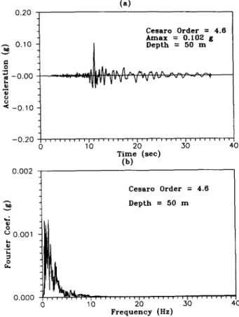
mean and the L-curve f o r the deconvolution problem 365 0.20 (a) 0.10 .9 ~ - 0 . 0 0 - O l O - 0 . 2 0 0 . 0 0 2 C e s a r o O r d e r = 4.6 A m a x = 0 . 1 0 2 g 0 10 20 30 40 T i m e ( s e e ) (b)

0

0.001 ..,. o 0.000 l C e s a r o O r d e r = 4.6 = 0 10 20 30 40 F r e q u e n c y (Hz)

Fig. 11. Basement motion deconvoluted from the contaminated ground surface motion by using Cesfiro regularization. (a)

Time history. (b) Fourier coefficient spectrum. o r

Tbg(f)

= cos(KsHs)• (6)

The amplitude function is defined by

Abg(f ) = ITbg(f )l.

(7)

When Ug(f) is given, the basement motion, Ub(f),

can be calculated by

Ub(f) = Ug(f) cos(gsHs)

(8)

and the time domain response, Ub(t), can be obtained by

FA1-5NS o //,~x\\ DHB06NS p=l.9g/cm 3 V,=68m/sec ~ , = 1 5 % o 0 m 6 m 1 1 m t 7 m 47 m D H B t t N S p=l•9g/cm 3 V=82m/sec ~,=10% O

oDHB17NS

p=l.g5g/cm' V,=159m/see ~ , = 7 % p=2.0g/cm 3 V=213m/sec {.=5% DHB47NS O Profile of LSST

Fig. 12. Soil profile of the far-field at the LSST site.

Fourier transform represented by

Ub(t ) = ~

Ub(fn) ei21rf"'•

(9)

1 1 = - - 0 0

In practical calculation, only the finite length of summation is taken, represented by

N

Ub(t)= Z eb(fn) ei2nf"'" (10)

n= -N

Comparing eqn (1) with (5), it can be seen that Tgb is the inverse of Tbg. A typical relationship of their amplitude vs frequency is shown in Fig. 2. The amplitude of convolution transfer function is greater than 1.0 in the low frequency range and decreases rapidly as the frequency becomes higher. On the other hand, the amplitude of deconvolution transfer function is lower than 1.0 in the low frequency range and becomes very large as the frequency becomes higher. Chen et al. l° defined the least frequency which

makes the amplitude of deconvolution transfer function always larger than one as the threshold frequency, shown in Fig. 2. Since the transfer function of convolution analysis has confined values, no serious errors will occur when the input motion is contaminated with noise. However, the deconvolution transfer function has very high amplitudes in the range where the frequency is much larger than the threshold frequency. This means that the transfer function can amplify any

(a) 0.3 0.2 0.1 .2 i 0.0 ",~ -0.1 -0.2 - 0 . 3 0 0.004 ~ 0 . 0 0 3 0.002 -= o.ool 0.000 Station : FAI-5NS Depth : 0 . 0 m 5 10 15 20 25 30 35 40 T i m e ( s e e ) (b) S t a t i o n : F A I - 5 N S D e p t h : 0•0 m

L~;III,I,II,I,I,I,,I,~,,I,I, I

0 5 10 15 20 25 30 35 40 F r e q u e n c y (Hz•)

Fig. 13. The input motion of the multilayered case• (a) Time history. (b) Fourier coefficient spectrum.

(7)

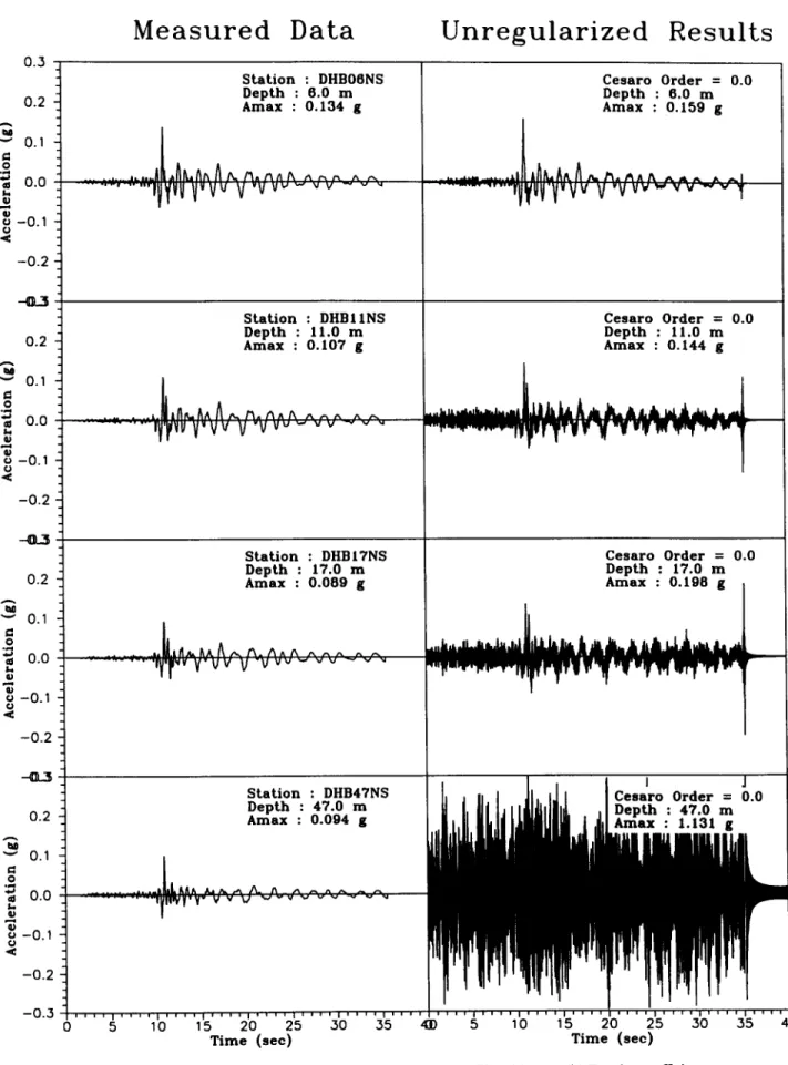
0.3

M e a s u r e d

D a t a

U n r e g u l a r i z e d

R e s u l t s

0 . 2 "~" 0.1 0 0 . 0 t., I0 o - 0 . 1 0 - 0 . 2 0 . 2 "-" 0.1 0 0 . 0 t.. ¢g o --0.1 - - 0 . 2 0 . 2 v 0.1 m 0 . 0 L I0 o - 0 . 1 0 S t a t i o n : D H B O 6 N S D e p t h : 6 . 0 m A m a x : 0 . 1 3 4 g . . .

I.J,ALAA A A.

f a ^ n ^ a ^ . . . . ' . . . wIyvv V ' v '~ V 'v ~ " ~ " , ' - ~ S t a t i o n : D H B I 1 N S D e p t h : 1 1 . 0 m A m a x 0 . 1 0 7 g

I

^

, . I I / ~ A ^ , ' , . . / % A ^ A ^ , - , ^ a ,-. wV~v V ' V V V "v v,, "-" " , ' ~ " " S t a t i o n : D H B I T N S D e p t h : 1 7 . 0 m A m a x : 0 . 0 8 9 g

..,.~tl1,,t,

ttxA,,~.A^hlJ

^ , - , , - ^ Iy, r , ,

V'VV

V " v v , , - - v v - . . ,, C e s a r o O r d e r = 0 . 0 D e p t h : 6 . 0 m A m a x : 0 . 1 5 9 g i . . . . "q'uV'V' v v V "v v , , , - , , , , - , , , , 'I C e s a r o O r d e r = O.O D e p t h : 1 1 . 0 m A m a x 0 . 1 4 4 g C e s a r o O r d e r = 0 . 0 D e p t h : 1 7 . 0 m A m a x : 0 . 1 9 8 g

"~'"~'"" ", trTtwW~l"Ir~l"'t w~"~

- 0 . 2 S t a t i o n : D H B 4 7 N S C e s a r o O r d e r = 0 . 0 D e p t h : 47.0 m Depth : 47.0 m ~ - 0 , 1 - 0 . 2 - 0 . 3 0 5 10 15 2 0 2 5 3 0 3 5 41) 5 10 15 2 0 2 5 3 0 3 5 T i m e ( s e c ) T i m e ( s e c )

Fig. 14. Comparison of m e a s u r e d d a t a a n d u n r e g u l a r i z e d results. (a) Time history. (b) Fourier coefficient spectrum.

(8)

Application of Ceshro mean and the L-curve for the deconvolution problem 3 6 7

Measured Data

0 . 0 0 4

,•.0.003

~ 0 . 0 0 2 I~ 0 . 0 0 1 0 . 0 0 0

"~0.003

1

L

0.002 o . o o l 0.00@ - - STATION : D H B O 6 N S D e p t h : 6 . 0 m S T A T I O N : D H B I I N S D e p t h : l I . O m

U n r e g u l a r i z e d R e s u l t s

C e s a r o O r d e r = 0 . 0 D e p t h : 6 . 0 m C e s a r o O r d e r : 0 . 0 D e p t h : I I . 0 m L _ , _ - _ : . . . , . . . . . ~ . ~ STATION : D H B I 7 N S D e p t h : 1 7 . 0 m

"-~o.oo3

v lg 0 0.002 i _ o 0 . 0 0 1 0.000 STATION : DHB47NS D e p t h : 4 7 . 0 m

~o.oo~

O 0.002

" k

0 . 0 0 1 0.000 . . . I ~ , ~ . . . I I I ! I I I l l l 5 10 15 2 0 2 5 3 0 3 5 ' F r e q u e n c y ( H z . ) C e s a r o O r d e r = 0 . 0 D e p t h : 1 7 . 0 m C e s a r o O r d e r = 0 . 0 D e p t h : 4 7 . 0 m 4]0 Fig. 14. C o n t i n u e d . 5 I 0 15 2 0 2 5 3 0 3 5 4 0 F r e q u e n c y ( H z . )

(9)

I v e~ o o9 ~> o 0 . 1 0 . 0 1 O r d e r a t t h e c o r n e r = 4 . 4 \ . . . . Order of Cesaro M e a n

Fig. 15. The constructed L-curve of the multilayered case. high frequency noise o f the contaminated input motion in deconvolution analysis.

In practical solutions, very few downhole records are available. Therefore, deconvolution analyses are usually used to calculate underground motions. The problem of high frequency amplification can not be avoided in the analysis. The next section will introduce a new regularization method to overcome the difficulty of high frequency amplification in deconvolution analysis.

3. R E G U L A R I Z A T I O N WITH T H E CESJ~RO M E A N T E C H N I Q U E

F o r the above mentioned ill-posed problem, regularization techniques, e.g. the T i k h o n o v method, 6 are often employed to transform the original problem into a well- posed one. The T i k h o n o v method can be used when the system is formulated in terms o f convolution type; however, it will introduce a double integral in the formulation. To avoid a large number o f calculations, the frequency domain approach is used in this paper, and hysteretic damping can be easily included. Therefore, we will propose a new regularization technique based on the theory o f the Cesfiro mean to regularize the ill-posed problem in the frequency domain. In the mathematical modelling for a physical problem, the series representation or integral representation for the solution is often assumed, and the governing equation in another domain can be equivalently obtained. Because some errors or the Dirac Delta function may be included in the solution, contaminated errors in the representation for solution will be present. In order to represent the solution more accurately, a regularization technique can reproduce the unknown solution more approximately. This is the reason why the Ces~ro mean is related to the reproducing kernel (Fejdr kernel)) 2

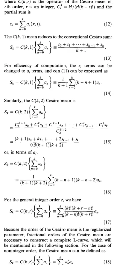
The general Ces~ro mean is defined as 2-5'8

Sk = C(k, r an

r t - ~ r - 1 S

_ c L + ( - ' s o + c L + ( - % + . . . + +

C~ +r

(ll)

where C(k, r) is the operator o f the Ces~tro mean o f rth order, r is an integer, C k = k t / ( r ! ( k - r)!) and the partial sum is

k

sk = Z an(x, t). (12)

n = 0

The C(k, 1) mean reduces to the conventional Ces~iro sum:

Sk = C(k, 1 an - k + l

(13) F o r efficiency of computation, the si terms can be changed to ai terms, and eqn (11) can be expressed as

S k = C ( k , 1) an = k + l E ( k - n + l ) a n '

n = 0

(14) Similarly, the C(k, 2) Ces~tro mean is

S k = C(k, 2 an

+ ' so + c s, + % + . . . + c?sk_ , + C: sk

C 2 k + 2

(k + 1)s o + kSl + . . " + 2Sk_ l + Sk

0.5(k + 1 ) ( k + 2) or, in terms o f ai,

Sg = C(k, 2) a n

k n = 0 )

1 k

-- ( k + 1 ) ( k + 2 ) Z ( k - n + 1 ) ( k - n + 2 ) a n .

n = 0

F o r the general integer order r, we have

{ kn~__

° } +(k)!(k+r-n)!

Sk = C ( k , r ) an - ~=o(-~C_n-~.(k~-~)!an.

(15)

(16)

(17) Because the order o f the Cesgro mean is the regularized parameter, fractional orders of the Cesfiro mean are necessary to construct a complete L-curve, which will be mentioned in the following section. F o r the case o f noninteger order, the Ces~ro mean can be defined as

Sk =-- C ( k , r ) a, = w~a,

t n = l n = l

(18) in which the weight is represented by

r ( k + 1)F(k + r - n + 1) (19)

w~ -- r ( k - - n + 1 ) P ( k + r + 1)

where P(x) is the G a m m a function of x. Equation (19) can be reduced to the weight in eqn (17) where r is an

(10)

Application of Ceshro mean and the L-curve for the deconvolution problem

369 integer. To understand the effect of the weight for each

basis

an,

the Cesfiro means of order 1, 5, 10, 20, 100 are shown in Fig. 3. It is seen that the Cesfiro mean has the physical meaning of a window function. The larger the order is, the lower is the weighting of a n treated. Therefore, if the Ces~ro window is applied for frequency domain deconvolution analysis, the amplitude of high frequency content can be suppressed, and the solution will be insensitive to the high frequency input error. From the viewpoint of signal processing, this method is the model of moving average (MA). Applying the Ces~tro mean to deconvolution analysis, eqn (10) can be replaced by

n=N

Ub(t)= Z WrUb(fn) ei27rf"t

(20)

n=-g

where

ub(t)

is a regularized solution instead of the unregularized solution

ub(t )

in eqn (10). Using the Fej~r theorem, 12 eqn (20) can be transformed to

1 f

Ub(t) = ~-~ J_~ K N ( t -

T)Ub(T )dT- (21)

where the reproducing kernel

Ku(t --

T) is

n=N

KN(t-- T) = Z

wr eiZTrfn(t-2)"

(22)

n=-N

For the case of order 1, the reproducing kernel is reduced to the Fejrr kernel as shown below:

1 sinZ((u + 1)(t - 7-)/2) (23)

Ku(t - 7-) = (N +

1) sin2((t - 7-)/2)

The diagram of the reproducing kernel is shown in Fig. 4 for increasing values of N. In application in the frequency domain, eqn (20) is used instead of eqn (21).

4. THE L-CURVE AND ITS APPLICATIONS Most numerical methods for treating ill-posed problems seek to overcome the problems associated with an ill-conditioned system by replacing the problem with a 'nearby' well-conditioned problem, whose solution approximates the required solution and, in addition, is a more satisfactory solution than the ordinary solution. The latter goal is achieved by incorporating additional information about the sought after solution, and often the computed solution should be smooth. Such methods are called regularization methods, and they always include a so-called regularization parameter, which controls the degree of smoothing. Now the order of the Cesfiro mean is chosen as the parameter of smoothness. A very convenient way of displaying the judgement of the optimal parameter is the L-curve, which was first presented by Lawson and Hanson. 9 In the L-curve, the

x-axis is the solution norm, and the y-axis is the residual norm. The former is the index of how smoothly the solution is treated, and the latter is the distance index between the predicted output and the real output. In the deconvolution of site response analysis, the order of the Ces~ro mean can be the index of smoothing, and the maximum acceleration of predicted output motion can be the index of closeness to the real output, i.e. using the order of the Cesfiro mean as the x-axis and the maximum acceleration as the y-axis. In this way, we can easily get a compromise between the regularization errors due to data smoothing and perturbation errors in measurements or other noise. According to the L-curve, the corner region is the appropriate choice for regularization parameter, i.e. the order of the Cesfiro mean.

5. NUMERICAL EXAMPLE - - SINGLE LAYER SOIL MODEL WITH ARTIFICIAL RANDOM ERRORS

To illustrate application of the Cesfiro mean and the L-curve on the ground motion deconvolution problem, the single layer ground model, shown in Fig. 1, is chosen as a representation example. It is assumed that the soil layer has a thickness of 50 m, a mass density of 2.0 g/cm 3, a shear wave velocity of 200m/s and a hysteretic damping ratio of 10%. According to eqns (1)-(7), the amplitude for convolution and deconvolution transfer functions can be plotted as shown in Fig. 2. From this figure, it can be seen that in the first, the second and the third modal frequencies of the system are located in the valleys of the amplitude curve of the deconvolution transfer function, which are equal to 1, 3 and 5 Hz, respectively. However, for frequencies larger than the threshold frequency (about 5.4 Hz), the deconvolution transfer function always has an amplitude greater than 1, and this increases very rapidly for higher frequencies. This is the cause of high frequency amplification in deconvolution analysis. Under these circumstances, even a small amount of high frequency noise contamina- tion in the input motion will result in serious error in the deconvoluted motion.

Suppose a normalized basement motion fib(t) is given as shown in Fig. 5(a). Its Fourier amplitude is shown in Fig. 5(b). The maximum acceleration of fib(t) is set equal to 0.1 g. By the direct convolution technique, the surface motion,

i~g(t),

and its Fourier spectrum can be obtained as shown in Fig. 6. The maximum acceleration of

i~g(t)

is 0.1615g. Comparing Fig. 5(b) with 6(b), it is found that the surface motion has larger amplitude in the low frequency range, concentrated at the modal frequencies of 1 and 3 Hz, and less high frequency content as compared to the basement motion.

To see the influence of high frequency noise in deconvolution analysis, the obtained surface motion,//g (t), was

(11)

0 . 3

M e a s u r e d

D a t a

R e g u l a r i z e d

R e s u l t s

0 . 2 " ' " 0.1 0.0 L., ca - 0 . 1 0 - 0 . 2 0 . 2 "G " - " 0.1 O 0 . 0 L . qD - - 0 . 1 - 0 . 2 0 . 2 " - " 0.1 I= .o m 0 . 0 L . o - 0 . 1 c a - 0 . 2 0.2 "-" 0.1 .o ,a 0.0 l,,, ca - 0 . 1 ¢.,) - 0 . 2 - 0 . 3 S t a t i o n : D H B O 6 N S C e s a r o O r d e r = 4 . 4 D e p t h : 6 . 0 m D e p t h : 6 . 0 m A m a x : 0 . 1 3 4 g A m a x : 0 . 1 3 7 g ... "'"*vq yvu V v v v V "v v,, - ,, ,, - v ~ ... rIVuv V ~ v v v "v v,, ,-- ,, ,, ~ v S t a t i o n : D H B I I N S D e p t h : 1 1 . 0 m A m a x : 0 . 1 0 7 g . . . Ll,n,,. ^^ A ~ ,-,. ,~,, ,, ,, . . . . . . . vIy'~v V'VV V "v v~ ~- ~ ~ ~ v S t a t i o n : D H B I T N S D e p t h : 1 7 . 0 m A m a x : 0 . 0 8 9 g . . . . a ~ a . t ~ x ~ A A . ^ ^ ^ i l ^ ^ ^ ^ .~ - " ~ ' r ' v ' v v v - v v,, - ~ v - ~ S t a t i o n : D H B 4 7 N S D e p t h : 4 7 . 0 m A m a x : 0 . 0 9 4 g C e s a r o O r d e r = 4 . 4 D e p t h : 1 1 . 0 m A m a x 0 . 1 1 3 g . . . ,,,,.. l ~ t , . L , . / ~ , , . A . ^ ^ A .,. . . . . . . .

'vv'F,v

y"

v v V -v vv

, - , , , , - - , C e s a r o O r d e r = 4 . 4 D e p t h : 1 7 . 0 m A m a x : 0 . 0 9 5 g . . . .LII~,.&A,,-.. ~. A . ^ ~. ^ ~ ~ ~ . ... l l ' " ~ r Y ' v v V V V V " " ' ~ ~ • C e s a r o O r d e r = 4 . 4 D e p t h : 4 7 . 0 m A m a x : 0 . I 0 0 g 1' ~IWV['V" V v V " " ' v v i i i i | 1 i i = i , i = | 1 i , W l iil~,ll , i i i v i , 0 g' % '~'5 '2b' '2'5' '~b' ' ~ ' ' ~ ' % " '1~" '2b" '2'5' '~b" '3~" '40 T i m e ( s e c ) T i m e ( s e c ) F i g . 16. C o m p a r i s o n o f m e a s u r e d d a t a a n d r e g u l a r i z e d r e s u l t s . (a) T i m e h i s t o r y . (b) F o u r i e r c o e f f i c i e n t s p e c t r u m .

(12)

0.004 '~0.003 "~°~0.002 ,~ o.oo~ O.OOO

~0.003

0.002 0.001 O.OOg

~0.003

v 0 0.002 k 0.001 O.OOO ' ~ 0 . 0 0 3

0

0.002 k = o.oo1 0.000

Application of Ceshro mean and the L-curve for the deconvolution problem

Measured Data

R e g u l a r i z e d R e s u l t s

371

!

S T A T I O N : D H B O 6 N S D e p t h : 6 . 0 m S T A T I O N : D H B I I N S D e p t h : tJ.0 m S T A T I O N : D H B I 7 N S D e p t h : 1 7 . 0 m C e s a r o O r d e r = 4 . 4 D e p t h : 6 . 0 m C e s a r o O r d e r = 4 . 4 D e p t h : 1 1 . 0 m C e s a r o O r d e r = 4 . 4 D e p t h : 1 7 . 0 m S T A T I O N : D H B 4 7 N S D e p t h : 4 7 . 0 m

L ~

l l l l l ' l l l [ ' l ' ' l ' l ' l l l l l l l l l l l l l l l l l l l l I ] l l l l

I I

0 5 10 15 20 25 30 35 C e s a r o O r d e r = 4 . 4 D e p t h : 4 7 . 0 m F r e q u e n c y ( H z . ) " i - ~ , ~ - ; , + i , ' ; , , T v ~ , , Y , ' , ' : - ; , . . . . ~,-,,'~ 4aD 5 10 15 20 25 30 35 40 F r e q u e n c y ( H z . ) Fig. 16. C o n t i n u e d .

(13)

superimposed by 3% r a n d o m error to simulate the probable errors in measurement, l° The contaminated surface motion, ~g(t), and its Fourier spectrum are shown in Fig. 7(a) and 7(b), respectively. To the naked eye, the difference between ~lg(t) and

iJg(t)

can not be seen. When the contaminated surface motion, ~g(/), is

used for deconvolution analysis if no regularization is considered, the basement motion obtained is as shown in Fig. 8. T o o much high frequency content is present, and the solution obtained is unrealistic.

When the above mentioned Cesfiro mean regularization technique is applied in deconvolution analysis with contaminated surface motion, ~g(/), we can construct the relationship between the maximum basement acceleration obtained and the order o f the Cesfiro mean, i.e. the L-curve, as shown in Fig. 9. In construct- ing the L-curve, the integer order o f the Cesfiro mean is used for the whole region at first, and the noninteger orders are then applied for the region near the corner o f the L-curve to reduce the computational effort. As expected from a mathematical point of view, a corner is present in the L-curve. When the Cesfiro order is at the left hand side of the corner, the maximum acceleration grows very fast and deviates very far from the accurate basement motion. If the Cesfiro order is larger than the corner value, the lower frequency content o f the deconvoluted motion will be over-decayed, and the maximum acceleration will become smaller. T o find a compromise between the smoothing and perturbation errors, the corner o f the L-curve is chosen as the optimal point. The appropriate order is 4.6. The original and regularized amplitude o f transfer functions are shown in Fig. 10. It can be found that the low frequency region o f the original transfer function is just slightly reduced by using the Cesfiro window while the high frequency region o f the transfer function has been suppressed very much. Therefore, the deconvolution result will be regularized to approximate the exact solution o f

ilb(t )

as shown in Fig. 11. Comparing Fig. 11 with Fig. 5, the two motions are almost the same except for a small difference in high frequency content. The application o f the Cesfiro mean in conjunction with the L-curve for the deconvolution problem is satisfactory.

6. N U M E R I C A L E X A M P L E - - M U L T I P L E LAYER S O I L M O D E L W I T H M E A S U R E D DATA

In this section, the deconvolution analysis o f the multilayered soil profile in Lotung, Taiwan, will be examined. The unregularized and regularized results computed by the S H A K E program will be compared with measured data from down-hole records from the LSST testing site in Lotung, Taiwan.

The soil profile o f the farfield at the LSST site was simplified to four layers as shown in Fig. 12, and the soil

properties o f shear wave velocities and damping ratios were deduced from the acceleration records measured by using the spectral ratio method in the study o f Chen. 1 These properties represent the equivalent parameters in the earthquake of 20 May, 1986 due to the nonlinear behavior of the soils. Station FA1-5 is located on the ground surface, and the downhole array o f DHB06, D H B l l , DHB17 and DHB47 is arrayed below the ground surface at depth 6, 1 l, 17 and 47 m. The NS component o f station FA1-5NS in the earthquake o f 20 May, 1986 was selected to be input motion. The regularized and unregularized motions underground were compared with the measured data o f down-hole stations for the same event.

The time history and Fourier spectrum o f the F A I - 5NS component are shown in Fig. 13. The wave form from Fig. 13(a) shows a major shock o f about 0.2g at time 11.3 s and periodic vibration between time 20 and 35 s. Figure 13(b) shows that the major frequency contents are lower than 5 Hz, and that the minor frequency contents are spread over 5-20 Hz. There is only a small contribution for frequencies larger than 20 Hz. The time histories of the down-hole array are shown in the first column o f Figs 14(a) and 16(a), the Fourier spectra are shown in the first column of Figs. 14(b) and 16(b), and the wave forms are similar to FA1-5NS in Fig. 13(a) with lower amplitude and lower frequency contents. This p h e n o m e n o n indicates that the ground record is highly contaminated with noise, which might not be convoluted from the basement. Based on the measured data at FA1-5NS as input motion, both regularized and unregularized solutions of the down-hole array can be deconvoluted by the S H A K E program in conjunction with or without the proposed regularization technique.

The unregularized deconvoluted results are shown in the second column o f Fig. 14. Figure 14(a) shows that tremendous errors occur in the motions at depths greater than 6m. These errors come from high frequency contents as shown in Fig. 14(b). It shows that the frequency contents are similar to the measured data while the high frequency contents deviate greatly with increasing depth. The tendency in this case is the same as that found by Chen. 1 F r o m the results of unregularized deconvolution analysis, the importance of the regularization technique is more obvious, and the results of regularized analysis are shown in the following. The regularization technique is incorporated into the S H A K E program to modify the transfer function of deconvolution. The L-curve is constructed according to the max acceleration at the deepest station, DHB47, as the y axis. The L-curve is shown in Fig. 15, and the order at the corner o f L-curve is 4.4. The regularized results using Cesfiro order 4.4 are shown in the second column o f Fig. 16(a) and 16(b). F r o m Fig. 16(a), we can find that the wave form can be simulated satisfactorily in comparison with the measured data when the depth o f calculation is not greater than 17m. Although the

(14)

Application o f Cesitro mean and the L-curve f o r the deconvolution problem 373 regularized results at station D H B 4 7 are similar to the

measured data including maximum acceleration and wave form, a few high frequency contents are still amplified as shown in Fig. 16(b). Comparing Fig. 16(b) with Fig. 14(b), we find that the high frequency contents have been suppressed by the Ces~ro mean.

7. C O N C L U S I O N S

The Cesdro regularization technique presented in this paper, together with the L-curve, plays a role in determining the optimal window which can maintain the system characteristics and make the system insensitive to the contaminating noise. Therefore, the long standing abstrusity o f determining the window by engineering judgement is solved by a theoretical window in conjunction with the L-curve. Two examples, a numerical case with artificial errors and a field case with data measured in Lotung, Taiwan, have been given to demonstrate the validity o f the proposed method.

A C K N O W L E D G E M E N T S

The authors are grateful to Dr. Yang-Jye Lee for valuable discussions.

REFERENCES

1. Chen, L. Y. Vertical propagation of seismic waves in soil layers. Master Thesis, 1988. Department of Civil Engineer- ing, National Taiwan University.

2. Hong, H.-K. & C h e n , J. T. On the dual integral representation and its application to vibration problems. In eds C. A. Brebbia and J. J. Rencis, Proc. 15th Int. Conf.

on B E M in Engineering, Worester, Massachusetts, 1993, pp. 377-392.

3. Chen, J. T. & Hong, H.-K. On the relations of hyper- singular kernel and divergent series in heat conduction problem using BEM. In Boundary Element Technology

VIII, eds H. Pina and C. A. Brebbia, Computational Mechanics Publication, Southampton, 1993, pp. 115-124. 4. Yeh, C. S., Hong, H.-K. & Chen, J. T. The application of

dual integral representation on the shear beam subjected to random excitations, Proc. 16th National Conf. Theoretical

and Applied Mechanics, Keelung, Taiwan (1992) (in Chinese), pp. 767-774.

5. Chen, J. T., Hong, H.-K., Yeh, C. S. & Chyuan, S. W. Integral represenations and regularizations for divergent series solution of a beam subjected to multi-support motion, in revised version, Earthq. Engng Struct. Dynamics, 1995.

6. Tikhonov, A. N. Regularization of incorrectly posed problems. Soviet Math. Dokl., 1963, 4, 1624-1627. 7. Schnabel, P. B., Lysmer, J. & Seed, H. B. SHAKE - - A

computer program for earthquake response analysis of horizontally layered sites. EERC Report-72/12, 1972 University of California.

8. Hardy, G. H. Divergent Series, (1949) London, Oxford University Press.

9. Hansen, Per Christian, Analysis of discrete ill-posed problems by means of the L-curve. S I A M Rev., 1992, 34(4), 561-580.

10. Chen, L. Y., Lee, Y. J. and Chen, C. H. Application of Cesdro mean and the concept of threshold frequency for ground motion deconvolution analysis. J. Chinese Inst. Civ.

Hydraul. Engng, 1994 (in Chinese).

11. Radziuk, J. The numerical solution from measurement data of linear integral equations of first kind. Int. J. Num.

Meth. Engr., 1977, 11, 729-740.

12. Korner, T. W. Fourier Analysis, 1988, Cambridge University Press, Cambridge.