Cooperation protocols in multi-agent robotic systems

Cooperation Protocols in Multi-Agent Robotic Systems

Department of Computer Science and Information Engineering, National Taiwan University, Taipei, Taiwan, R.O.C.

[email protected] [email protected]

Abstract. Multi-agent robotic systems are useful in many practical applications. For some tasks, such as holding a conference, cooperation among agents are necessary. For other tasks, such as cleaning a room, multiple agents can work in parallel for better performance. This paper provides help-based (HCP) and coordination-based (CCP) protocols for controlling agents to accomplish multi-agent tasks. The HCP utilizes efficient negotiation to coordi-nate agents into groups. The CCP improves overall performance by exchanging local knowledge among agents and making decisions in parallel. A reactive and modularized agent architecture was employed to implement the proto-cols. Since each protocol is embedded into the architecture, it is efficient and effective. In addition, the protocols are deadlock-free. The protocols were utilized to solve the Object-Sorting Task, which abstracts two characteristics of tasks: parallelism and cooperation. The experimental results showed that 1) both HCP and CCP are stable under different workload; 2) the protocols can effectively utilize the agent-power to achieve super-linear improvement; 3) The CCP is better than the HCP in both performance and speedup.

Keywords: multi-agent cooperation, deadlock handling, multirobot systems, multi-agent tasks, distributed auto-nomous robotic systems

1. Introduction

Multi-agent systems employ multiple agents to solve problems. Nuclear power plants, space or undersea ex-ploration, and manufacturing systems are typical ap-plication domains. The advantages of a multi-agent system include cost, parallelism, fault-tolerance, and modularity. In particular, parallel performance and co-operation inside tasks are the main interests of the emerging multi-agent robotic systems.

Some tasks can be executed in parallel for better performance. Tasks such as painting a wide wall or cleaning rooms can be partitioned into several parts, each of which is then assigned to an agent. If all agents work independently, i.e., no resource contention or goal conflicts, the performance is linearly speeded up. Otherwise, if there is resource contention (e.g., short of paintbrushes or brooms) or conflicts (e.g., agents have different favorite colors), the performance speedup will be sublinear. On the other hand, some other tasks

re-quire explicit cooperation among the agents, e.g., con-ferences and moving a heavy equipment.

In order to move a heavy equipment, a robotic agent must call for help and wait for the arrival of its partners, then they can start to move the equipment. For telecon-ferences, a couple of communication channels must be reserved and kept available for discussion among the attendants. In the information retrieval domain, a query may require many information servers to provide their information or knowledge. The query engine waits to collect all the information, then prepares the answer for users. All the situations explicitly require the coopera-tion among agents. The Object-Sorting Task described in the paper is an abstraction of these tasks. It consists of both parallelism and cooperation characteristics in which explicit cooperation is required to accomplish the task.

There has been much research in multi-agent ro-botic systems. Hackwood and Beni’s research on swarm robotics demonstrated large scale cooperation

176 Lin and Hsu

in simulation (Hackwood and Beni, 1992). Brooks et al. (1990) developed the lunar base construction robots by using a set of reactive rules implemented on subsumption architecture (Brooks, 1986). By us-ing the schema-based architecture (Arkin, 1989), Arkin (1992) demonstrated that cooperation between robotic agents was possible even in the absence of communi-cation. It simplified the design of an agent because there was no communication between agents. On the other hand, it may be inefficient due to the lack of communication. Arkin et al. (1992, 1993) assessed the impact on performance of a society of robots in a forag-ing and retrieval task when simple communication was introduced.

Some researchers proposed mechanism to create the foundation of multi-agent robotic systems. Fukuda’s CEBOT system (1989) showed the self-organizing be-havior of a group of heterogeneous robotic agents. Asama et al. (1989) proposed the ACTRESS archi-tecture for connecting equipment, robots, and com-puters together to compose autonomous multi-agent robotic systems by designing underlining communica-tion architecture. Wang (1995) proposed several dis-tributed functional primitives on disdis-tributed robotic systems.

Some other researchers worked on solving multi-agent tasks. Mataric (1992) addressed the problem of distributing a task over a collection of homogeneous mobile robots. Collective homing and flocking tasks were experimented. Balch and Arkin (1994) investi-gated the importance of communication in robotic so-ciety. They evaluated the performance of three generic multi-agent tasks (forage, consume, and graze) un-der different types of communication. Alami et al. (1995) coordinated the multiple-robot navigation with a plan-merging paradigm for the task of transporting containers in harbors. All the mentioned tasks can be accomplished with one agent alone. However, there are many real world tasks that require explicit cooperation among agents and cannot be achieved by any single agent alone, such as moving a heavy equipment. Agah and Bekey (1995) studied the effects of communica-tion by simulated robot colonies on the fetch-and-carry task in which an object may require one or two robots for movement. Their work addressed the communica-tion radius issue rather than cooperacommunica-tion issues such as coordination and deadlocks. On the contrary, Lin and Hsu (1995a) proposed a cooperation protocol with deadlock-handling schemes for tasks that may require any number of agents.

Since these tasks require cooperation and coordina-tion among agents, the achievement of tasks will be accidental if agents work independently. Tasks cannot be done unless agents cooperate and coordinate their behaviors. Therefore, it is necessary to have a cooper-ation protocol that allows multiple agents to help each other in the problem solving process.

To solve a multi-agent task, either centralized or distributed approaches can be employed. A central-ized model uses a powerful agent to plan and sched-ule the subtasks for every agent. This control agent has global knowledge concerning the environment and the problems. It can deliberately plan for better perfor-mance, e.g., optimal solutions. However, for tasks with NP complexity, the centralized approach is impracti-cal. Furthermore, the control agent must be powerful enough to achieve satisfactory performance. High de-sign complexity, high cost and low reliability are the other drawbacks of centralized approach.

On the other hand, a distributed approach decreases design complexity and cost, while increasing the reli-ability. Agents are autonomous and equal. An agent plans for itself and communicates with the others in order to accomplish the global task. Since every agent interacts directly with the environment, it is reactive. However, each agent has only local knowledge of the task and the environment. Hence, it cannot make the best decision of the global task alone. Furthermore, ne-gotiation and social cooperation rules for conflict res-olution are required to coordinate among them.

One distributed approach is to let each agent work alone. Whenever an agent cannot achieve its goal by itself, it requests help from the others. Moreover, every agent always offers help when it can. This is help-based cooperation. It is simple and effective in achieving the overall task. Its problems include: too many helpers for an agent is a waste; too many agents requiring help will cause a deadlock; some agents obtain help more often than the other agents (unbalanced load) ; and local knowledge limits the system performance.

Another approach is to let agents work together. For a given task, agents coordinate a global plan for per-forming the task by exchanging their local knowledge. It is coordination-based cooperation. With enough in-formation, a task can be optimally achieved. Moreover, each agent can optimize its decisions. The problems of this approach include overhead due to coordina-tion, complexity in choosing optimal decisions, and the amount of storage for saving the exchanged infor-mation.

In this paper, two distributed approaches, the help-based cooperation protocol (HCP) and the coordi-nation-based cooperation protocol (CCP), were uti-lized to solve multi-agent tasks with a modularized and reactive agent architecture. The Object-Sorting Task (OST) was applied to demonstrate the approaches. Section 2 introduces and discusses the OST. The agent architecture for implementing the protocols is pre-sented in Section 3. The HCP, CCP, associated dead-lock handling, and implementation are described in Sections 4 through 6. Finally, simulation and exper-imental results are shown in Section 7. In addition, Section 8 provides several issues for implementing the proposed protocols to real robots.

2. The Object-Sorting Task (OST)

The Object-Sorting Task provides an abstraction model for the type of tasks which consist of both parallelism and cooperation characteristics in which explicit coop-eration is required to accomplish the task. The OST was showed to be a NP-complete problem for finding the optimal performance (Lin and Hsu, 1995b). This section presents its definition, search complexity, and problem analysis.

2.1. Definition

Let O = {o1, . . . , oM} be a set of stationary objects that are randomly distributed in a bounded area. Every object, oi = (li, di, ni), is associated with an initial location li, a destination location di, and the number ni of agents for movement. An object oi can be moved only if there are at least niagents available to move it. An object is a large object if ni > 1, or it is a small object if ni = 1. Let R = {r1, . . . , rN} be the set of agents and nmaxbe the maximal number of agents to

move any single object, an object-sorting task can be completed only if N is not less than nmax. Agents search

for objects and move them to their destinations. When all the objects have been moved to their destinations, the task is finished.

Typical application examples of OST are foraging and retrieval, explosives detection and handling, AGV dispatching for components transportation in FMS, and surveillance, etc.

There are many models associated with different strategies to do the task, e.g., any object is assigned to agents at random, the movement of objects are

con-trolled by a predefined precedence, and the action of agents are all central-controlled, etc. No matter what operational model and strategies are arranged, its so-lution can be represented by the sequence of objects moved by each agent. This sequence is called Agent-Object Sequence (AOS). For each agent ri, let si j∈ O represent the j th object moved by ri(and its partners). An AOS is represented by the form:

r1: s11s12· · · s1k1

r2: s21s22· · · s2k2 · · ·

rN : sN 1sN 2· · · sN kN

For example, the number of objects that r1 involved

to move is k1 and the sequence is s11s12· · · s1k1. Let

I(si j) be the initial location of si j, and D(si j) be the destination of si j. The cost of si jis defined as

ci j= ai j+ wi j+ mi j where

ai j: the cost of ri moving from I(ri) to I (si 1) when j = 1, or the cost of ri moving from D(si( j−1)) to I(si j) when 1 < j ≤ ki.

wi j: the cost of riafter reaching I(si j) and waiting for enough agents to move si j.

mi j: the cost of ri moving si jfrom I(si j) to D(si j). All ai j, wi j, and mi j are defined by its model, e.g., a model may use distance to define them. Let fi be the cost of ri moving from D(si ki) to I (ri), i.e., return to

its initial location. The cost of agent ri is defined as

CRi= Ã X j ci j ! + fi

For example, CR1 is the cost of r1 spent on its k1

objects and returning to its initial location. Obviously, the maximum CRi(1 ≤ i ≤ N) is the maximum cost to achieve the AOS. Hence, the cost of the AOS is defined as

Cost= Max CRi, 1 ≤ i ≤ N

Generally speaking, an agent searches for objects, co-ordinates with the other agents for handling objects, and cooperates to move objects. The cost of an applied model is the maximum cost among all the agent costs.

178 Lin and Hsu

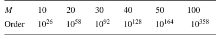
Table 1. The order of search space for N= 10 agents.

M 10 20 30 40 50 100

Order 1026 ₁₀58 ₁₀92 ₁₀128 ₁₀164 ₁₀358

2.2. Search Complexity

Finding an optimal solution of OST is an NP-complete problem. The search space can be depicted from the search process of Algorithm Optimal-OST. It lists all object sequences, then assign agents to the objects for each sequence. There are M! object sequences from M objects, and C(N, ni) assignments for each ob-ject oi, where C(k, r) is the number of r-combinations from k. Hence, the search space is M!(PC(N, ni)),

1 ≤ i ≤ M. Let E(C(N, i)) be the mean of

C(N, i), 1 ≤ i ≤ N. The search space becomes M!(E(C(N, i)))M. Table 1 lists the order of search spaces for different number of objects when N = 10 agents.

Algorithm. Optimal-OST.

1. FOR each permutation of objects o1, . . . , oMDO (1) Let the object sequence be s1, . . . , sM. (2) FOR each si = (li, di, ni) in s1, . . . , sMDO

a) Let C(r) represent all the r-combinations from the agent set{r1, . . . , rN}.

b) FOR each combination of C(ni) DO Assign the agents to the object si. (3) Compute the cost of s1, . . . , sM.

2. The optimal solution is the object sequence com-bined with the assigned agent, which has minimal cost.

2.3. Assumptions

The system assumptions are the following: 1. Agents are homogeneous mobile robots.

2. Agents have no prior knowledge about the environ-ment. They know the environment around them only after they have detected it.

3. Agents are cooperative.

4. Agents can communicate through reliable broadcast or point-to-point channel.

5. Every agent is autonomous and has the basic capa-bilities:

• object recognition. It can identify the other

agents, the obstacles, and the target objects.

• navigation and obstacle avoidance. It can move

from one location to a specified location.

• object handling. It can move an object alone or

with the other agents. 2.4. Problems

To solve the OST, several problems need to be ad-dressed.

1. Search. All the objects must be found in order to achieve the task. The most intuitive way is to let agents search the entire area so that they can find all the objects. How do they search efficiently? 2. Coordination. How do agents coordinate each other

for assigning themselves to any found object? That is, for a given object, which agents should work together to move it? and who makes the decision? 3. Deadlocks. When each agent autonomously selects

an object and none of the selected object has enough agents for movement, a deadlock occurs. A coordi-nation solution must solve the problem.

4. Load balance. How is all the load of the task dis-tributed to agents? If some agents are busying in search or handling objects while other agents are idle, the performance will be poor. More load bal-ance stands for better performbal-ance.

5. Cost balance. The smaller the maximum cost of the agents is, the better performance is. Intuitively, more balanced cost may reduce the maximum cost of the agents.

6. Termination. How do every agent realize that the global task has been accomplished?

The OST consists of two subtasks: search for objects and object movement. Moreover, the OST includes two types of task characteristics: parallelism and coopera-tion. The search subtask can be easily paralleled. Let the entire area be equally partitioned into N subar-eas, then each subarea is assigned to one agent. The movement subtask also can be paralleled if multiple agents can move multiple objects simultaneously. Ob-viously, This is a cooperation problem because agents must coordinate themselves to control the parallel per-formance. Another characteristic is cooperation: an object may require several agents for its movement. Hence, it is necessary to have cooperation protocols that allow multiple agents to help each other in the problem solving process.

Many protocols can be utilized for the OST. One effective and reactive protocol is the help-based proto-col. In this model, every agent searches the objects in its subarea. When an agent finds a large object, it calls for the other agents’ help. Then, it selects its partners from the agent willing to offer help. After the arrival of its partners, they start to move the object.

Another improved protocol is the coordination-based protocol which lets an agent broadcast the object data when it finds an object. After having searched the entire area, agents coordinate to plan an agent-object sequence for object movement. This model stores ob-ject data for obtaining better performance through coor-dinating overall object movement. Although response of object movement may be slower, the global perfor-mance is better than the help-based protocol.

All the proposed protocols are designed and imple-mented on the agent architecture described in the next section.

3. Agent Architecture

At the bottom of the agent architecture, each agent has the basic behaviors such as navigation, object handling, etc. Based on the behaviors, the architecture presented in the section focus on functionality. The overall func-tion of each agent is controlled by cooperafunc-tion proto-cols which are realized by finite state automata (FSA). Furthermore, the global FSA is distributed into sev-eral functional modules which perform subsets of the global FSA simultaneously.

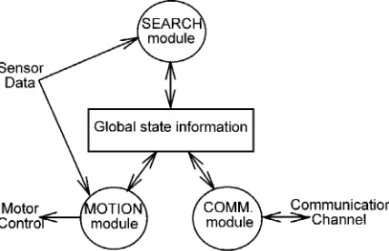
For the OST, the system architecture of each agent is shown in Fig. 1. The search module, communica-tion(comm.) module and motion module are all finite

Figure 1. The architecture of each agent.

state automata coordinated through a global state. They share and change the state information according to their state functions. The search module searches for objects, identifies their destinations and required num-ber of agents. The motion module performs the function of object movement alone or with other agents. The communication module communicates with the other agents in order to cooperate with them.

Advantages of the architecture are described in the following:

• Simplicity. The global FSA is very complex.

Com-pared with a central module controlling all the state transition, the architecture is more simple, clear and fast for implementation.

• Reactivity. Agents react and cooperate quickly

be-cause cooperation protocols are realized into state transition functions and each module handles only a subset of the global FSA.

• Intra-agent Distributed Control. Functional

separa-tion for each agent makes the intra-agent distributed control. All state transitions are distributed into the modules and a single transition is done only by one module. The modules can run concurrently or simul-taneously based on multiprocessor or uniprocessor platform. The communication between modules is through the shared global state information.

• No fixed Inter-agent Control. Agents communicate

with each other only through the communication system. The inter-agent control can be designed for different kinds of purpose. Depending on ap-plications, it may be central control or distributed control.

• Flexibility. It is ease to add a new functional

mod-ule to the agent architecture. Additional functions can be performed by the agents if the corresponding modules are included in the architecture.

4. Help-Based Cooperation Protocol (HCP) The HCP defines how and when an agent requests help, how and when the other agents offer help, as well as deadlock handling, in order to coordinate the agents for accomplishing the task.

The working area is partitioned into disjoint N sub-areas, and each subarea is assigned to an agent. Each agent exhaustively searches its subarea. It requests help once it finds a large object, then selects its partners from the agent willing to offer help. After there are enough agents arriving at the found object, they carry the object

180 Lin and Hsu

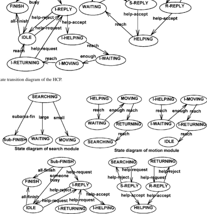
Figure 2. State transition diagram of the HCP.

Figure 3. Each module’s state diagram of the HCP.

to its destination. Since each agent is independent and autonomous, simultaneous selection of partners by sev-eral agents may cause a deadlock. Sevsev-eral schemes are utilized to handle deadlocks.

The global state diagram representing the HCP is showed in Fig. 2, and the state diagrams of each mod-ule are showed in Fig. 3. Each circle is a state and

a thread represents the state transition driven by the event on the thread. The I-states in the figures are uti-lized to distinguish the agents having finished their sub-tasks from the agents not having finished their subsub-tasks. For example, an agent is in RETURNING state or in I-RETURNING state after it has helped out. The agent will be in SEARCHING after RETURNING state while

it will be in IDLE state after I-RETURNING state when it reaches its destination.

4.1. Cooperation Strategies

An overview of the HCP is described with the following cooperation strategies:

1) Request-help strategy. An agent broadcasts a help message when it finds a large object. It is called a requiring-help agent.

2) When-help strategy. The strategy determines when to offer help. An agent accepts a help message only when it is in SEARCHING, (I-)RETURNING or IDLE states (whose states will be described in next subsection). Otherwise the message is queued for later processing.

3) Select-help strategy. It enables an agent to decide which agent has the most urgent need for help when there are many agents requiring help. An agent se-lects the nearest to offer help. That is, select the agent with minimum approaching cost. An agent that responds to a help message is called a will-help agent.

4) Select-partner strategy. A requiring-help agent ri must choose suitable partners if there are more will-help agents. The selected partners are called will- help-ing agents, and ri is called helped agent. An agent chooses the nearest will-help agents as its partners, i.e., the agents with minimum approaching cost. 5) Load-balancing strategy. It is considered in two

parts. One part is to uniformly distribute agents into equal-partitioned area. Another part is embed-ded in the select-partner strategy. When an agent needs help from n agents, there may be m will-help agents such that m is greater than n. The load-balancing strategy enables the agent to select the first n nearest agents, who will receive an accept message. The other will-help agents will be rejected by reject messages.

6) Deadlock-free strategy. Deadlocks are the situa-tion that all the agents are in WAITING state or I-WAITING state. First, the agents in(I-)WAITING state detect the deadlocked situation (which will be discussed in detail in Section 5), then they broadcast blocked messages to exchange their state informa-tion and break down the blocked situainforma-tion by com-paring their priorities. The lower priority agents will enter(I-)HELPING state and go to help the highest priority agent.

4.2. Search Module

The search module searches for the objects and iden-tifies their destinations in the SEARCHING state. It changes the state to MOVING if the object is small, or to WAITING and broadcasts a help message if the object is large.

Since agents are independent, they don’t know in which situation the others are. When an agent has com-pletely searched its subarea, it does not mean the system task is done. It is necessary to have a protocol to let agents know when the task is done. When an agent r has accomplished its subarea, it broadcasts a sub-fin message and comes into Sub-FINISH state. Any other agent whose subtask is not yet finished will reply a busy message to the agent r . If r receives a busy message, it enters into IDLE state. Otherwise, it means all the subtasks are finished and r will broadcast an all-finish message. All the agents in IDLE come into FINISH state after receiving the finish message, i.e., the system task is finished.

4.3. Motion Module

Agents in MOVING state is moving an object to its destination, and will change the state to RETURNING after having moved the object to its destination. When in RETURNING state, an agent is returning to its sub-area and the motion module will change the state to SEARCHING after arrival. An agent in HELPING state is walking toward a helped agent, and will change the state to WAITING when arrival. If there are enough agents for carrying the object, the agents in WAITING will change the state to MOVING.

After an agent has finished its subtask, it enters IDLE state and returns to its base location. The agent will be in I-HELPING when it is moving to a helped agent, and will change the state to I-WAITING when arrival. If there are enough agents to move the objects, the agents in WAITING state will change the state to I-MOVING. When it has moved the object to the desti-nation, the agent comes into I-RETURNING, then the state is changed to IDLE when it has returned to its base location.

4.4. Communication Module

When receiving a help message in SEARCHING or RE-TURNING states, the communication module replies a

182 Lin and Hsu

will-help message and changes its state to S-REPLY or R-REPLY. If the requiring-help agent accepts the will-help message, it sends back an accept message to the agent, otherwise, it sends a reject message to reject the help. When receiving an accept message, the commu-nication module changes the state to HELPING. When receiving a reject message, the communication module returns to its previous state.

An agent in IDLE state stays in its base location and waits for help message in order to help the others. The mechanism is the same as described above.

5. Deadlock-Handling Schemes

Here is a deadlock situation using the HCP. There are 4 agents R= {r1, r2, r3, r4} and two objects o1, o2with n1 = n2 = 3. If r1 finds object o1 and r2 finds

ob-ject o2 at the same time, r3 and r4 will receive help

message from both r1and r2. If r3 chooses to help r1

and r4chooses to help r2according to the select-help

strategy, all the agents will enter the WAITING state. A deadlock occurs. We say{o1, o2} causes the system coming into a deadlock. Here is a fact coming from the strategies used.

Fact 1. If a set of objects will cause the system com-ing into a deadlock, they are large objects and found at the same time.

Explanation: Assume there is a set of objects K =

{oi| oi ∈ O, ri∈ R, oiwas found by riat time ti} such that the system comes into a deadlock. Since a small object requires only a single agent to move, it will not cause a deadlock. So oiis a large object if oi ∈ K . For any oi, oj ∈ K, i 6= j,

Case 1: ti< tj. Since rj was in SEARCHING before tjaccording to the state diagram, rjmust have been a will-help agent to ri and rejected by ri according to the when-help strategy and the state diagram. So rihad enough partners to move oi. The result is that oi should not be in L. So this case is impossible. Case 2: ti> tj. Similar to Case 1, it is impossible also.

So ti = tj. That is, the large objects causing system blocked are found at the same time.

Since the small objects will not cause a deadlock, we fo-cus on the large objects. Let Lt= {oi| oi ∈ O, rj∈ R, s.t., oi was found by rj at time t}, |Lt| = k, be a set of large objects, and rt(oi) denote the agent rj such that oi ∈ Lt and oi was found by rj at time t. Gt =

{rt(oi) | oi ∈ Lt}. Remember oi = (li, di, ni), and ni is the required number of agent to move oi. Let Ft =

{r | r ∈ R, r 6∈ Gt} be the set of agents which don’t find large object at time t . Since the objects causing a deadlock must be found simultaneously, the following discussion uses a fixed t . Ltis referred to as L, rt(oi) is referred to as r(oi), and Gtis referred to as G. We as-sume N ≥ nmax. If k= 1, the other agents can help the agent in G and the system will not come into a deadlock. So a deadlock may occur if k> 1. It is obvious that a deadlock will occur if for all oi ∈ Lt, ni > |F| + 1.

There are three approaches for handling deadlocks: deadlock prevention, deadlock avoidance, and dead-lock detection. Which deaddead-lock-handling approach is suitable greatly depends on the application. Based on the strategies provided in previous section and a lit-tle modification, we propose three schemes to handle deadlocks for the object-sorting task.

5.1. Deadlock Detection

In what follows, we will present the analysis for any agent in(I-)WAITING state to detect the deadlock situ-ation. Lemma 1 shows that a deadlock can be detected by checking the number of objects causing agents to stay in the (I-)WAITING states if global knowledge about the agent state is available. In a distributed en-vironment, Theorem 1 allows each agent to identify a deadlock based only on local information.

Let MTT be the maximum travel time between any two locations in the bounded area, and Wt,u = {o | o

∈ Lt, some agent is in WAITING or I-WAITING state at time t+ u due to o}, so Wt,0= Lt·Wt,uis referred to as Wuin the following discussion.

Lemma 1. Given|Wu| > 0, the system is deadlocked iff

|Wu+2MTT| = |Wu|.

(That is, the system is not deadlocked iff |Wu+2MTT| < |Wu|.)

Proof: The “only if” part is trivial and obvious. Next we consider the if part: given|Wu+2MT T| = |Wu|. The agents are partitioned into the following sets according to their current states, except the FINISH state which means that the task has been finished:

MOVE= {r ∈ R, r’s

HELP= {r ∈ R, r’s

state is HELPING or I-HELPING} WAIT= {r ∈ R, r’s

state is WAITING or I-WAITING} AVAIL= {r ∈ R, r’s

state is SEARCHING or

RETURNING or I -RETURNING or IDLE} TEMP= {r ∈ R, r’s

state is S-REPLY or R-REPLY or I-REPLY or SUB-FINISH}

Each state in TEMP is a transit state and can be ignored. Given|Wu| > 0, i.e., WAIT set is not empty, if the system was not deadlocked at time t+ u, the agents in AVAIL can offer help immediately and the agents in MOVE or HELP may offer help in the future. If they can help to move an object at time t+ u + v other than enter WAIT, then|Wu+v| < |Wu|. We consider the case in each set starting from the time t+ u: 1) HELP set: When an agent in HELP set reaches the

object, either it enters MOVE set if there are enough agents to move the object or enters WAIT set. Ob-viously, an agent stays in HELP state no more than one MTT. So the maximum time for these agents to reach and move an object in Wuis one MTT. 2) AVAIL set: Every agent in the set is a will-help

agent. If the agents in AVAIL are accepted by the requiring-help agents, they enter HELP set. So the maximum time for these agents to reach and move an object in Wuis a MTT.

3) MOVE set: The time that an agent stays in MOVE and enters AVAIL set is no more than one MTT. Af-ter that, the agent enAf-ters HELP set immediately if there is requiring-help agent. So the maximum time for these agents to reach and move an object in Wu is 2MTT.

So the maximum time for the agents not in WAIT to reach and move an object in Wu is 2MTT. On the other hand, they all enter the WAIT set if they cannot move any object in Wuin 2MTT. That is, the system is

deadlocked if|Wu+2MT T| = |Wu|. 2

Theorem 1. For object-sorting tasks, a deadlock is that all agents keep staying in WAITING or I-WAITING states. Let MTT be the maximum travel time be-tween any two locations in the bounded area. When any agent stays in WAITING state or I-WAITING state for 2(N − 1) MTT, the system is deadlocked.

Proof: The system is deadlocked if all the agents find large objects at the same time, i.e.,|W0| = N. If it is not the case, i.e.,|W0| < N. From Lemma 1, the sys-tem is not deadlocked at t+ 2MTT if |W2MTT| < |W0|. In the worst case:|W0| = N − 1, |W2_(N−1)MTT| = 0 if the system is not deadlocked at t+ 2(N − 1)MTT. That is, all the objects in L have been moved, and there is no agent in WAITING or I-WAITING due to the objects.

So if an agent stays in WAITING state or I-WAITING state for 2(N − 1)MTT, all the agents must be in either WAITING state or I-WAITING state and the system is

deadlocked. 2

This scheme is very simple and effective. How-ever, it may be inefficient because the deadlock detec-tion time is propordetec-tional to the number of agents. The system performance will degrade when the number of agents increases. To avoid unnecessary waiting, let an agent r broadcasts an is-blocked message every 2MTT when staying in(I-)WAITING, and the other agents not in(I-)WAITING reply with not-blocked message. If r receives any not-blocked, it keeps waiting, otherwise, it has detected a deadlock situation. This improvement can detect a deadlock quickly once a deadlock occurs. Nevertheless, it introduces redundant message trans-mission.

5.2. Object Priority

This scheme prevents deadlocks by the following parts:

• It assigns a unique priority to each object.

• Select-help strategy is modified. An agent selects

the agent having found the highest priority object.

• Select-partner strategy is modified. An agent selects

its partners by first considering their states are not in

(I-)WAITING, then shorter distance.

• When-help strategy is modified. An agent in (I-)

WAITING state also can offer help if it is not the agent having found the object with the highest priority. An object has a higher priority if it is nearer to its destination. In our two-dimensional experimental en-vironment, for example, the priority of an object is determined by comparing the following order: 1. the distance between the object and its destination, 2. x-coordinate of the object,

184 Lin and Hsu

Since there is no more than one object having the same

(x, y) coordinates, different object has different

pri-ority. The scheme guarantees that the selection of a requiring-help agent to offer help will not cause a deadlock when an agent is available to offer help. The modified when-help strategy is for the situation when ni > |F| + 1 for all oi∈ L.

This scheme is very simple and easy for implementa-tion. Nevertheless, many redundant messages are trans-ferred for replying to the help coming from higher priority agents, or rejecting the will-help agents which are more than required.

5.3. Feasible Sequence

This scheme utilizes the concept of feasible sequence and associated algorithms in order to guarantee that se-lecting an agent to offer help doesn’t cause a deadlock. Meanwhile, it has additional advantages:

• It eliminates the redundant messages transferred. • It is load-balancing.

• It can improve the system performance.

Definition: Feasible sequence. A feasible sequence is a permutation sequence s1, . . . , si, . . . , skof L, si∈ L, 1 ≤ i ≤ k, such that s1is moved to its destination by the agents in F and r(s1), then s2 is moved to its destination by the agents in F, r(s1), and r(s2), . . ., and finally skis moved to its destination by all agents.

For example, assuming R = {r1, r2, r3, r4}, L =

{o1, o2}, G = {r1, r2}, n1 = 3, n2 = 2, a feasible

se-quence may be o1, o2or o2, o1. If n1= 3, n2= 4, the

feasible sequence is o1, o2only.

Theorem 2. For object-sorting tasks, a deadlock is that all agents keep staying in WAITING or I-WAITING states. Let L be the set of objects found at the same time. Any deadlock which may be caused by L can be avoided if there is a feasible sequence in L.

Proof: Fact 1 states that L may cause a deadlock. However, there is a feasible sequence in L. Assume s1, . . . , sk is the feasible sequence, we can let s1 be

moved to its destination first, then s2, . . . , and let sk be moved to its destination at last. Since all the ele-ments in L are moved to their destinations, the deadlock which may be caused by L has been avoided. 2

If there is a feasible sequence in L, the agents can moved these objects according to the sequence. Fur-thermore, they can distribute themselves to different objects such that more than one object can be moved simultaneous and increase the performance. It is im-plemented in Algorithm load-balancing.

If there is no feasible sequence in L, the select-help strategy must be modified to avoid coming into a deadlock. In addition, the agents in G may need to exit WAITING state to help each other. For exam-ple, assume R = {r1, r2, r3, r4}, L = {o1, o2}, G =

{r1, r2}, r(o1) = r1, r(o2) = r2, n1 = 4, n2 = 4, and

the sorted sequence of L is o1, o2. Though there is no feasible sequence, both r3 and r4 can select r1 as

the helped agent. Besides, r2must exit WAITING state

and go to help r1to avoid a deadlock. After o1having

been moved to its destination, the agents can continue to move o2. In order to implement the scheme, the

select-help strategy is modified to the following: Step 1. If k= 1, the agent in G is the selected agent.

Otherwise, continue the next step.

Step 2. Use algorithm find-feasible-sequence to check if there exist a feasible sequence in L.

Step 3. If there is a feasible sequence in L, use al-gorithm load-balancing to select the helped agent. Otherwise, select the agent according to the order of the sequence s1, . . . , sk sorted in algorithm find-feasible-sequence. That is, if will-help r(s1) is re-jected, try r(s2), etc.

Let I(oi) = i be an index function for oi ∈ L. Algorithm find-feasible-sequence will find a feasible sequence in L if there is a feasible sequence in L. Algorithm. Find-feasible-sequence.

Step 1. Sort L by keys ni and agent priority to an sequence s1, . . . , sk. First sort by key ni with non-decreasing order. If ni = nj, compare the agent priorities of r(oi) and r(oj) to determine their order. Step 2. C= N − k. FOR 1≤ i ≤ k DO j= I (si); IF C+ 1 ≥ nj THEN C = C + 1. ELSE

mark si+1, . . . , skas the unsatisfied sequence, the result is no feasible sequence,

exit.

Algorithm. Load-balancing.

Step 1. Initialize the current number of agent, Ci, for all oi ∈ L to 1. Step 2. j= 1. FOR 1≤ i ≤ N DO IF ri ∈ F THEN l= I (sj); IF Cl< nlTHEN

IF i is equal to my id. THEN rlis the selected agent, exit. ELSE

Cl= Cl+ 1; IF Cl= nlTHEN

j = j + 1.

The agents in F also need some modification for their behavior when they stay in(I-)WAITING state. If there is a feasible sequence, they can stay(I-)WAITING state and wait for help. While there is no feasible sequence, the agents in G must exit(I-)WAITING state to help each other in order to avoid a deadlock.

Step 1. Use algorithm find-feasible-sequence to check if there is a feasible sequence in L.

Step 2. If there is no feasible sequence in L, and the object found by itself is in the marked unsatisfied objects si+1, . . . , sk, select the helped agent accord-ing to the order of the sequence si+1, . . . , sk. That is, if will-help r(si+1) is rejected, try next one in the sequence, etc.

The sorted sequence is kept by all agents and is referred when they can help the others till all objects in L are moved.

6. Coordination-based Cooperation Protocol (CCP)

The HCP utilized simultaneous subarea search for par-allel performance, and cooperation protocol for solving the coordination, deadlocks, and termination problems. The protocol is realized into each agent’s state tran-sition function so that agents reacted and cooperated quickly. Nevertheless, the performance of OST can be further improved.

One characteristic, mentioned in Section 2.4, of the OST is parallel movement of objects. In HCP, an ob-ject is processed immediately once it is found, which

limited the global knowledge of agents. Hence, the de-gree of parallel movement depends on the dynamics of environment. That is, agents cannot make cost-optimal decisions. The CCP has been developed to address this issue.

Like HCP, the CCP uses equal partition of the work-ing area for parallel search. However, instead of re-questing help once an object is found, every object information is broadcast and saved when received. With the overall object information, each agent makes its optimal decision and negotiates with the others for a global agent-object sequence (AOS) which defines ev-ery agent’s object sequence. Then, each agent moves objects according to its object sequence. In order to efficiently resolve conflicts, social rules are employed into a coordination algorithm from which decisions are obtained by each agent independently so as to minimize negotiation overhead.

6.1. Coordination Points

A coordination point specifies the time when agents should start coordinating the AOS for the found objects. The simplest way is to start a coordination process after having searched the entire area. Since the CCP requires every agent to save the information of found objects, the storage demand will expand with the increasing number of objects.

However, coordination can start during subarea search under storage constraints or in order to reduce storage demand. Several events can be utilized to ac-tivate a coordination process, such as having found a certain number of objects, a part of area searched, or a fixed time interval if there is a common clock. The frequency of coordination is specified by the coordina-tion interval (CI), e.g., coordinacoordina-tion is activated every 100 time units (CI= 100) or every 20 objects found (CI= 20). The unit of CI employed in the paper is a certain number of objects found, since it is more natural to the OST.

Since it is possible that more than one object are found at the same time, the actual number of objects found may be more than the CI when a coordina-tion process begins. Agents must have the same object set for each coordination process. Under such circum-stance, either the exactly CI number of higher priority objects or all found objects attend the current coordi-nation process. Object ID can help to determine the object priority.

186 Lin and Hsu

6.2. Object Identifications

In order to clearly identify objects during coordina-tion, a consistent representation of objects is necessary. Generally, assigning a unique ID for each object is appropriate. However, various assignment methods should be suitably applied under different situations. Several methods are discussed:

1) Predefined attributes: Object IDs are predefined so that it can be identified by agents. An object can be identified from its outside look, size, sym-bol, or initial location. For example, a two dimen-sional coordinate can determine the order of object IDs by comparing x-coordinate then y-coordinate in order.

2) Coordinator: Where there is no way to specify a predefined object ID, this method can be applied. Every object found is reported to the coordina-tor, then the coordinator broadcasts the ID to the others.

3) Other more complicated distributed algorithms (e.g., Lamport, 1986; Wang, 1993) concerning the order of discrete events may be employed when the coordinator method is unsuitable.

6.3. Coordination Algorithm

The OST is a NP-complete problem, thus there is no polynomial time algorithm for overall optimal AOS. The utilized coordination strategy is based on balanced cost and greediness. Algorithm Coordination depicts it. All agents invoke this algorithm to coordinate their individual object sequence.

At first, every agent selects a local cost-optimal ob-ject and broadcasts its selection. Among the selected objects, the best cost-optimal object is scheduled, i.e., enough agents are assigned to it. Finally, every assigned agent updates its cost and location. The process is re-peated until all objects are scheduled.

Algorithm. Coordination

1. Every agent selects its current cost-optimal object, and broadcasts to the others. Let the selected objects be s1, . . . , sk, 1 ≤ k ≤ N.

2. Select the best cost-optimal object, Opt, among the selected objects.

(1) FOR each object in s1· · · skDO

• Let the current object be oi = (li, di, ni).

• FOR each agent rj DO

Let C Aj be the accumulated cost of rj, and C Rj be the cost of rjto reach oi. Ci j= C Aj+ C Rj

• Mi= the nith smallest cost from Ci 1, Ci 2, . . . , Ci N

(2) Opt= the object with minimum Mi 3. Assign agents to Opt, and update data.

Let Opt be op= (lp, dp, np).

Assigned agents are the npagents with smaller cost Cpi, 1 ≤ i ≤ N.

IF I am one of the assigned agents THEN (1) append Opt to my object schedule;

(2) accumulate my cost with (Mp+ the cost from l to d);

(3) my location= d.

4. Repeat from Step 1 until all object has been sche-duled.

Obviously, this approach is cost balance because selec-tion strategy is to choose the agents with smaller cost. Besides, it is deadlock-free from the two facts: there is a consistent object order in every agent’s object se-quence and there are enough agents assigned to every object.

Since every agent selects one object for coordina-tion at a time, the number of selected objects is at most N . For each selected object, it requires time complex-ity O(N) to calculate all costs of agents. So, the cost for scheduling an object is O(N2). Since there are M objects, the complexity of algorithm Coordination is O(M N2).

There are several differences between the HCP and CCP.

1. Task partition: The HCP partitions objects and as-sign each part to an agent while the CCP partitions the search task only.

2. Object assignment: An object is assigned to which agents is determined by cooperation strategies in HCP while by coordination strategy in CCP. 3. Handling objects found: An agent deals with an

object at a time ( request help, select partners, then move object) in HCP while an agent broadcasts the object information in CCP when an object is found.

For the CCP, negotiation of the object sequence is delayed till having found a number of objects or having finished the search task.

4. Sequence of handling objects: The sequence of han-dling objects in HCP is determined by the order that an agent finds an object while by negotiation in CCP. The exhaustive search algorithm determine the or-der of object found.

5. Knowledge: The HCP makes decision with local knowledge other than global knowledge in CCP. 6. Object data: The CCP requires that every agent

keep all the object data while not in HCP.

6.4. Implementation

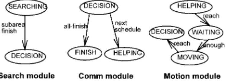
The transition diagram of CCP is shown in Fig. 4; and Fig. 5 shows the transition diagrams of each mod-ule. At first, agents start searching in SEARCHING state, broadcast the information (initial location, desti-nation location, and required number of agent) of each object found. After an agent has finished its search sub-task, it broadcasts this message and enters DECISION state. During searching, agents will start a coordina-tion process if they reach a coordinacoordina-tion point, then exchange local optimal selections and run

Coordina-Figure 4. State transition diagram of the CCP.

Figure 5. Each module’s state diagram of the CCP.

tion algorithm to obtain the global AOS. Coordination and object handling can perform simultaneously. Ev-ery agent’s object sequence is stored in its object queue. When an agent enters DECISION state, it picks the next object from its object queue and changes to HELPING state for going toward the target object. When the agent arrives at the object, its state becomes WAITING. If there are enough agents for carrying the object, they enter MOVING state and move the object to its desti-nation. They each repeat the movement cycle until all assigned object tasks having been accomplished.

If the object queue is empty when an agent in DECI-SION and not all objects are scheduled in the AOS, the agent will wait for an assigned object task. This is for considering the cases when agents are in coordination or specially when CI= M, i.e., coordination will start only if all the area has been searched. An agent enters FINISH state when all objects have been scheduled and its object queue is empty.

7. Simulation

The object-sorting task was simulated in a multi-strategy simulator developed on Sun workstation with graphic user interface showing the task execution. The simulator is a testbed for testing different cooperation protocols on the OST. Figure 20 shows a sequence of snapshots for a task execution before its start, during the execution, and after its completion.

7.1. Simulation Environment

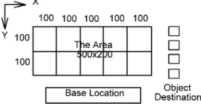
The working area was equally partitioned into N sub-areas, and each subarea was assigned to an agent. The area is represented in a two-dimensional coordinate system, e.g., 500× 200. The partition of the area is represented by a m× n notation, m in x-axis direction and n in y-axis direction. For example, 5× 2 parti-tion means that the area is equally partiparti-tioned into 5 subparts in x-axis direction and 2 subparts in y-axis direction, as showed in Fig. 6. In the experiment, the area was 500× 200. Figure 6 shows the map used in the simulation for N = 10 agents with 5 × 2 partition. The partitions for different number of agents N used in the experiment are shown in Table 2.

Each agent searches for the objects in its subarea and moves the objects to their destinations. The per-formance was evaluated with the number of time steps. The following code fragment describes the actions per-formed by the agent at each time step.

188 Lin and Hsu

Table 2. Partition and the number of agents.

N 1 2 4 8 10 20 30 40 50

Partition 1× 1 1× 2 2× 2 4× 2 5× 2 5× 4 6× 5 8× 5 10× 5

Figure 6. The simulation map for 5× 2 partition.

Figure 7. Move directions.

Figure 8. Sensor ranges.

for each agent i ,

do the search module of agent i ; do the motion module of agent i ; do the communication module of agent i . The area is a grid area, and the agents can only move to one of the four locations from a location in a time unit as the Fig. 7. The agents can sense the objects located in the grids adjacent to the agents as the Fig. 8. The agents may use any exhaustive search method to search their subarea. In this experiment, a row-major method was used. They start search from the initial location,

the (0, 1) location of their subarea, to the right side boundary, and search the first three rows which are under the sensor range. When they have reached the right side boundary, they search the second three rows and change the search direction from right to left. When they has reached the left side boundary, they change the search direction from left to right and start searching the next three rows. The search repeats until the subarea has been searched.

Each message has one time unit delay, i.e., a message sent at time t will be received at t+ 1. Computation can be performed with movement of agents, thus the computation time is ignored in performance evaluation. Each object was randomly generated for its destina-tion, initial locadestina-tion, and the number of required agents. This experiment generated 10 sets of object data for each number of object M using nmax= 10. All object

sets were run for N = 10, 20, 30, 40, and 50. When the object sets were applied to N = 1, 2, 4, and 8, then nmax was set to N and all the ni were proportionally adjusted in order to accomplish the task.

The experiment was run by varying the number of agents N , and the number of objects M. For a given number M of objects, the execution time was the av-erage of the execution time run from the 10 generated object sets of M. The performance was evaluated by comparing the execution time under different number of agents and different number of objects. The actual execution time performed by the HCP was represented by H , and C for the CCP. The reference execution time were the upper bound, U , and the estimated lower bound, L.

The upper bound is the execution time of the pro-fessional furniture movers (PFM) which is a centrally-controlled model. In PFM, all the agents start together searching the area for objects. When they find an ob-ject, a group of agents are assigned to move the object. The remaining agents continue searching objects and assigning groups. If the main search group is too small to move an object, they will wait. After the assigned groups have delivered their objects, they return back to join the main search group. The main group would finally become large enough to move the object after the assigned groups return one after another. In or-der to simplify the problems of group separation and

combination for the model, each assigned group is as-sumed to return to the location where its object was found. When a group returns to the previous location, it follows the same search path of the main group so that the two groups will meet eventually. The process is repeated till they have searched the entire area and delivered all the objects.

The estimated lower time is the execution time un-der the operation model that the other agents are always available for offering help when an agent finds a large object. The available agents are assumed to be in the central point of their subareas. An agent chooses its partners which are closer to it, i.e., with minimum cost. The execution time of each agent is its subarea search time and all the processing time for the objects located in its subarea. The processing time of the object j lo-cated in the agent i is the wait time for the arrival of all its partners, the movement time for object j , and the return time from the destination of the object j to the initial location of j . So, the estimated lower bound is the maximum time among the execution time of all the agents. L = Max TAi TAi = TSi+ X j TOi j TOi j = TWi j+ TMi j+ TRi j where

L: estimated lower bound.

TAi: the total execution time of agent i . TSi: the time for agent i to search its subarea. TOi j: the processing time of object j located in

the subarea of agent i .

TWi j: the maximum wait time of object j for all the helping agents of agent i .

TMi j: the time that agent i moves object j to its destination.

TRi j: the time that agent i returns from the

destination of object j to the previous location.

7.2. Simulation Results of HCP

The experimental results of HCP showed that 1) The protocol is stable and reliable under a spectrum of workload. 2) The execution time increases linearly with the number of objects. 3) Increasing the number of agents can significantly decrease the waiting time and improve the performance.

Figure 9. The execution time of HCP for N= 10 agent.

At first, the actual execution time, H , was com-pared with the estimated lower bound and upper bound. Figure 9 shows the relationship between the execution time and the number of objects for N= 10 agents. Intu-itively, as the number of objects to be moved increases, the execution time, either estimated or actual, will in-crease. In general, the upper bound model needs more time to do the task because it moves the objects sequen-tially.

When the workload is light, it takes less time to wait for help. As a result, the performance of the coopera-tion protocol approaches the lower bound. The agents search their subareas simultaneously and move objects simultaneously if they don’t need to wait for the others. Under heavy workloads, there are more demands for agents and each agent must spend more time to wait for help. Since every agent is often busy, the de-gree of concurrency is decreased. The agents have a tendency to group together and move objects sequen-tially. If most objects require a large number of agents to move, the system behavior will approach the upper bound in which objects are moved one by one. Further-more, most agents will find objects and need help when they return to their subareas due to heavy workloads. Under this situation, agents will waste time in return-ing to subareas and goreturn-ing to help move the next object. Hence, the performance of HCP will be equal to (even worse than) the upper bound under heavy workload situations, e.g., 200 objects.

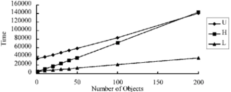
In comparison, the HCP is much better than the upper bound model in the experiments summarized in Fig. 10 which shows the U , H , and L for N= 50 agents under different number of objects. When using more agents, the performance of all three models has been improved. The more agents do the task, the faster the task is fin-ished. Moreover, the HCP is better than the upper bound model even under heavy workloads. It showed that the HCP can effectively utilize the agent power.

Second, the execution time for different number of agents under the same object sets were compared.

190 Lin and Hsu

Figure 10. The execution time of HCP for N= 50 agents.

Figure 11. The execution time of HCP for N= 1, 2, 4, 8, and 10 agents.

Figure 11 shows the execution time for N = 1, 2, 4, 8, and 10 agents. The workload is proportionally adjusted for any M by adjusting the number of required agents for each object. When the number of objects increases, the execution time increases linearly with it for all N . It shows that the cooperation protocol is very stable under different workloads. When the estimated upper bound and lower bound are considered again, we can find that U , H and L overlap when N = 1. It is very clear that both the upper bound model and the lower bound model work the same as the proposed model if there is only one agent to do the task and nmax= 1.

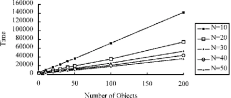
Finally, Fig. 12 shows the speedup effect of the HCP. When the generated object sets are applied to N ≥ 10 agents, the execution time decreases with the increasing number of agents. It shows that the protocol can effec-tively utilize the benefit from increased agent-power. The speedup is high when N is changed from 10 to 20, and it is low when N is changed from 40 to 50. Ini-tially the waiting time is significantly decreased when using more agents. If there are usually enough agents available to help out whenever a large object is found, the benefit from increasing N will be a smaller subarea for each agent.

The deadlock handling schemes have been tested on the cases with deadlocks and without deadlocks,

res-Figure 12. The execution time of HCP for N = 10, 20, 30, 40

and 50 agents.

pectively. In the cases with no deadlocks, the deadlock detection scheme (DD) spends less time than the object priority (OP) scheme on 56% of the cases with 0∼ 3% faster. On the other hand, in the deadlock cases, OP is a little bit better than DD with 1∼ 4% faster in 72% of the deadlock cases. The results indicate that choosing the nearest partners is better for general cases. However, the strategy does not prevent deadlocks, and therefore must pay for the overhead of deadlock detection, e.g., 2MTT. Selecting a highest priority object can prevent deadlock but it loses the geometric advantages, e.g., shorter distance.

Since the feasible sequence (FS) scheme exchange object data and assigned themselves with a load-balancing approach, it has the best performance in the three deadlock handling schemes. FS is faster than DD in 83% deadlock cases with relative 0∼ 2.5% im-provement. On the other hand, the scheme has a higher complexity for implementation. In summary, none of the three sets of strategies is better for all cases. In cases with rare deadlocks, the deadlock detection scheme is adequate. For a frequent deadlock situation, either ob-ject priority or feasible sequence scheme is better.

7.3. Simulation Results of CCP

The experiment includes: the performance comparison between the HCP and CCP in both execution time and speedup, and the comparison of different coordination intervals. The results showed that 1) The CCP has the same features as the HCP, i.e., stable behavior and speedup effect. 2) The performance of CCP is better than the HCP, and the CCP has better speedup effect. 3) Furthermore, CI is flexible in choice.

Figure 13 shows the execution time of CCP when N = 2, 4, 8, and 10 agents. When the number of ob-jects increases, the execution time increases linearly with it for all N . It shows that the CCP is very stable

Figure 13. The execution time of CCP for N = 2, 4, 8, and 10 agents, with CI= 1.

Figure 14. The execution time of CCP for N= 10, 20, 30, 40, and 50 agents, with CI= 1.

under different workloads. When the generated object sets are applied to N≥ 10, the execution time decreases with the increasing number of agents as showed in Fig. 14.

Table 3 further lists the speedup ratio relative to the execution time of N = 10 agents. Let the execution time of N agents be CN. The speedup ratio SN is:

SN = (C10/CN)(10/N)

Compared with the HCP’s speedup ratio showed in Table 4, the CCP has significant effect on speedup. It shows that the CCP can effectively utilize the increased agent-power.

For most cases with M> 30, the speedup is linear or superlinear. There is obvious improvement on jects movement because more agents make more ob-jects movement in parallel. For example, assume there are three objects requiring 5, 6, and 7 agents respec-tively. They will be moved in sequence when N = 10 while moved in parallel when N= 20. The speedup ratio is 3. On the other hand, for small number of ob-jects, e.g., M= 1, more agents decrease the search time

Table 3. The CCP speedup ratio relative to

N= 10. Number of object, M Number of agents, N 10 20 30 40 50 1 1 0.82 0.67 0.61 0.53 10 1 0.95 0.88 0.85 0.82 20 1 1.01 0.96 0.92 0.88 30 1 1.04 1.02 0.99 0.93 40 1 1.05 1.03 1.04 1.00 50 1 1.04 1.04 1.04 1.00 100 1 1.08 1.09 1.12 1.09 200 1 1.09 1.14 1.15 1.15

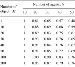
Table 4. The HCP speedup ratio relative to

N= 10. Number of object, M Number of agents, N 10 20 30 40 50 1 1 0.81 0.65 0.57 0.48 10 1 0.88 0.69 0.68 0.59 20 1 0.89 0.83 0.75 0.61 30 1 0.93 0.80 0.76 0.65 40 1 0.91 0.84 0.76 0.67 50 1 0.91 0.85 0.72 0.69 100 1 1.00 0.90 0.83 0.76 200 1 0.95 0.87 0.79 0.76

due to smaller subarea. But, there is no obvious im-provement on object movement since there is no sig-nificant increasing parallelism. Hence, the results also provide a useful reference when adding more agents for speedup. Where there is a superlinear speedup, adding more agents can be beneficial. Under sublinear speedup condition, the benefit of adding more agents is not as significant.

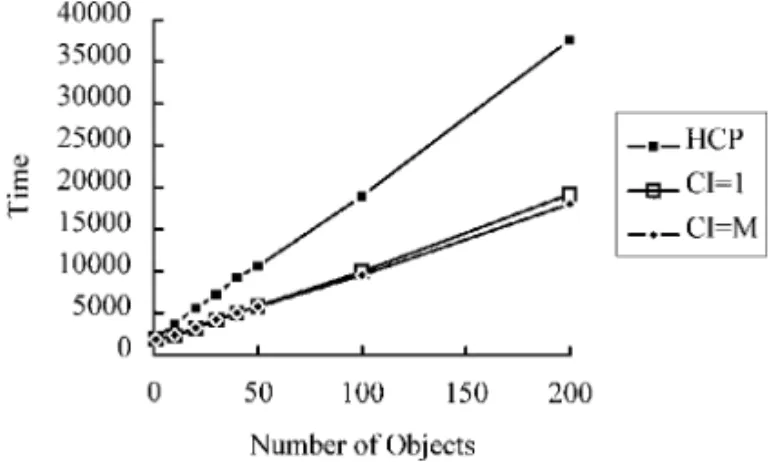
Next, Figs. 15 and 16 typically present the com-parison between HCP and CCP under N= 10 and 50 agents, respectively. The CCP results include both CI= 1 and CI = M, i.e., coordination activated once finding an object or after having searched the entire area. No matter what CI value is chosen, the CCP is always superior to the HCP. In addition, the CCP is obviously better than the upper bound model by com-paring Figs. 15, 16 with Figs. 9, 10. Through global coordination and cost-balanced strategy, the CCP can efficiently perform the OST.

192 Lin and Hsu

Figure 15. Comparison of execution time for HCP and CCP when

N= 10.

Figure 16. Comparison of execution time for HCP and CCP when

N= 50.

Figure 17. Execution time for different coordination interval when

N= 10.

Finally, the effect of different CI is showed in Figs. 17 and 18 where CI= 1, 10, 20, 30, 40, 50, 100, and 200. Larger CI can make better decisions due to holding more information for coordination, and smaller CI requires more coordination processes. Hence, a larger CI has better performance than a smaller CI in general. On the other hand, smaller CI requires less storage and is faster in generating the object sched-ule for movement. In addition, the difference between

Figure 18. Execution time for different coordination interval when

N= 50.

CI= 1 and CI = M becomes smaller when there are more agents such as N = 50 in Fig. 18. Hence, CCP is flexible in choosing CI.

8. The Path to Implementation

This section describes communication and uncertainty issues when implementing these cooperation protocols in real robots. Variability in the proposed approach is illustrated by simulation on the object-drop uncertainty and variable message delay.

8.1. Communication

The messages in the proposed protocols are important. They should not be lost. For example, if a help message broadcast to the other agents is lost, the requiring-help agent may not be able to move its object since there may not be enough number of willing-help agents. If an agent’s selection message is lost when broadcast-ing its selected object to the others, the coordination algorithm will fail in running the overall object sched-ule. Hence, a reliable communication system must be utilized for the cooperation protocols. A reliable communication system can guarantee that every mes-sage sent should reach the destination agent. The well known TCP/IP is a reliable communication protocol. It can be found in many popular systems such as Unix or Windows.

In the absence of reliable communication systems, additional mechanisms can be appended to the com-munication module. Each message sent is monitored by acknowledgment and retransmission mechanisms. When an agent receives a message, it sends a message back to the sender to acknowledge the received mes-sage. The sender will retransmit the message if it is not acknowledged by its receiver within the predefined time duration.