地理研究 第63期 民國104年11月
Journal of Geographical Research No.63, November 2015 DOI: 10.6234/JGR.2015.63.02
採用廣義極值分布對馬來半島極端降雨進行統計模擬
*A statistical modeling of extreme rainfall in Peninsular Malaysia
using the Generalized Extreme Value (GEV) distribution
黃燕儀
a翁叔平
bYuen-Yi Ng Shu-Ping Weng
摘 要
本研究採用時間序列為 1971-2007 年,馬來西亞水利灌溉局 22 個自動降雨測站之日降水資 料,取年最大值及季最大值對馬來半島極端降雨的變化進行分析,進一步擬合廣義極值分布模式 (GEV),計算出極端降雨的重現水平。根據研究結果顯示,半島東部地區的年最大降雨強度最 高,而半島中部地區為低強度的極端降雨,但是在近年來有上升的趨勢,表示此區在未來可能面 臨過去所未曾遭遇到的極端洪災事件。在季節分析上,中部地區春秋二季在未來可能遭受更頻繁 的水患事件,而北部地區在秋季時則可能面臨乾旱的災害。本研究以GEV 分布模式推估出 50 年 和 100 年極端降雨的重現水平。在參數估計上,根據最佳配適度檢定結果顯示最大似然估計法 (MLE)的配適度優於線性動差估計(LM)。我們發現半島西部和東部極端降雨重現水平的推估 值具有明顯的空間差異,其中東岸地區重現水平的變化明顯高於半島西部地區,表示西部地區極 端降雨實際觀測值很容易就超越了百年重現水平。上述的研究結果也透露出 GEV 分布模式對於 半島西部地區極端降雨的重現水平估計依然難以掌握,雖然在配適度上得到了不錯的配適成效, 這值得讓我們做進一步地思考。在極端降雨的空間分布特徵上,這樣的結果也暗示了近年馬來半 島極端降雨的趨勢在空間分布上的轉變。 關鍵詞:極端降雨、廣義極值分布(GEV)、重現期、時空變化Abstract
In this study, we have used the maximum daily rainfall data from a total of 22 automatic rainfall stations obtained from Department of Irrigation and Drainage Malaysia (DIDM) during 1971-2007. We
* This paper was originally presented in May, 2015, at the 19th International Geography Conference of Taiwan.
a Ph.D. Student, Department of Geography, National Taiwan Normal University ([email protected]). b Associate Professor, Department of Geography, National Taiwan Normal University.
have made use of the annual and seasonal maximum daily rainfall data to analyze extreme rainfall in Malaysia. We have also applied the generalized extreme value (GEV) distribution to model the occurrence probability of extreme rainfall in Peninsular Malaysia. The results showed that the greatest rainfall intensity was found in the east coast of Malaysia, while the lowest extreme rainfall intensity was found in the west central areas. Besides, our study also highlights a positive trend of extreme rainfall event that occurred at west central region in recent year. This result also suggests a likely increase of extreme flooding events in Malaysia in the coming years. For seasonal analysis, it is suggested that a rising flood disaster would possibly be affecting west central areas during the spring (MAM) and autumn (SON), while the northern part of Peninsula would probably suffered from the drought disaster during SON. We have also used the GEV distribution to calculate the return value for the 50-year and 100-year return periods. The maximum likelihood estimation (MLE) is suggested to be the best estimation in this study based on the result of goodness-of-fit. In this study, we have also noticed an apparent difference between the western and eastern parts of Peninsular Malaysia on the variation scale of return level, in which the variation recorded in the eastern region was greater than that of the western region. In addition, the observed rainfall level in the western region had exceeded the 100-year return level estimation. Our results suggest that deliberation is needed in the use of the GEV distribution for the estimation of the return levels of extreme rainfall in the western part of Peninsular Malaysia. For the spatial pattern of the extreme rainfall, our results also suggest that there is a shift in the spatial distribution of the extreme rainfall in recent years.
Keywords: Extreme rainfall, Generalized Extreme Value (GEV), Return period, spatial-temporal variability
Introduction
In recent years, an increment in precipitation that occurred around the world is associated with climate change. Furthermore, the frequency and scale of disasters, e.g. extreme floods, landslides and mudflows, would expand with an increase in extreme rainfall events. It could also cause severe damage to the human society, resulting in human casualty, infrastructure destruction, economic stagnation, financial loss, disease outbreak, etc. Several studies have raised concern on the issue of extreme rainfall in Malaysia (e.g. Juneng et al. 2007; 2010; Wan Zin et al. 2009; 2010; Zakaria et al. 2012) in response to the extreme flooding associated with the global warming. In respect of this, the study and analysis of extreme rainfall would be important in facilitating effective flood management.
Nowadays, both dynamic simulation and statistical analysis were used in the study of extreme rainfall. The use of dynamic simulation could help in reconstructing the behavior of extreme rainfall events in an efficient way. However, the simulation results would not be able to perfectly forecast every possible extreme rainfall event due to highly variable environmental conditions. In addition, the complexity in the modeling process itself would also lead to myriad technical uncertainties and hence
causing more challenges to dynamic simulations. Statistical analysis is an alternative approach for the study of extreme rainfall, in which historical weather data were use for analysis, interpretation, organization, and induction of the spatial-temporal distribution and the trend of the extreme rainfall events. In the extreme rainfall study, the extreme value theory is a popular method used in the research of extreme rainfall. It is used to establish the probability distribution model and to estimate the return level of the extreme rainfall.
Extreme value theory is a method of statistical analysis concerning small probability events. In the past, the extreme value theory had gained considerable ground to become a major concept in the probability theory. It has been widely applied in many fields, for instance, financial marketing (e.g. McNeil and Frey 2000), risk and insurance management (e.g. Berlant et al. 1996), earthquake (e.g. Lavenda and Cipollone 2000), hydrology and hydraulic analysis (e.g. Martins and Stedinger 2000), atmospheric science, etc. In atmospheric science, extreme value theory has been applied in the sea levels analysis (e.g. Sobey 2005), temperature (e.g. Zwiers et al. 2011), precipitation (e.g. Feng et al. 2007), and so on.
In the summer of 1972, Rapid City of the South Dakota in the United State was landed with severe flood disaster. It had caused a tremendous loss of property and life. Most people have referred to the disaster as a "once-in-a-century" event. Hershfiels (1973) indicated that there was a common inadequacy in the public understanding of the term “once-in-a-century” in frequency analysis. He pointed out that the extreme rainfall frequency analysis played an important role in the prediction of flood disaster and had used the Gumbel distribution to estimate the probabilities of extreme rainfall in Rapid City. Thereafter, Gumbel distribution has always been used by some investigators in their extreme rainfall analysis (e.g. Pagliara et al. 1998). However, many other studies were skeptical of the Gumbel distribution model and argued that it tended to underestimate the maximum extreme rainfall (Wilks 1993; Koutsoyiannis and Baloutsos 2000; Coles et al. 2003; Coles and Pericchi 2003; Koutsoyiannis 2004). Koutsoyiannis and Baloutsos (2000) indicated that the 3-parameter Generalized Extreme Value (GEV) distribution was more suitable than the 2-parameter distribution such as Gumbel distribution to interpret the upper tail of a probability distribution of extreme rainfall through the annual maximum daily rainfall data spanning a period of 136 years from 1860-1995 that was provided by a meteorological station in Athens.
The progress of the application of extreme value theory to extreme rainfall was extending to various other distributions, for example, Parida (1999) indicated that the generalized 4-parameter Kappa distribution has the ability to fit the extreme data well and it also could take the form of several underlying distribution including the 2-parameter and 3-parameter distributions. Furthermore, Park et al. (2001) and Park and Jung (2002) have used 5-parameter Wakeby distribution and 4-parameter Kappa distribution, respectively, to model the extreme rainfall in South Korea during the summer. However, Nadarajah and Choi (2007) were disapproval of these distributions, arguing that those were not extreme value distribution and there was no theoretical basis to model the extreme rainfall based on these
distributions. In Malaysia, Zalina et al. (2002a; 2002b) and Wan Zin et al. (2009) used various types of distribution models such as the Gumbel, Gamma, GEV, generalized normal, GPD, Pearson type 3, etc. to model the extreme rainfall distribution in Malaysia. However, it is still debatable whether using annual maximum daily rainfall in all types of distribution would lead to a questionable result.
In this study, we used the generalized extreme value (GEV) distribution, a classical extreme value theory that has the flexibility of the other three major types of distribution models proposed by Jenkinson in 1955. GEV is a typical extreme value distribution model based on the annual maximum, or block maximum value data collection (Chu et al. 2009). According to previous studies, 3-parameter GEV distribution model is widely used for extreme value analysis in different countries like United State (e.g. Chu et al. 2009), China (e.g. Feng et al. 2007), South Korea (e.g. Nadarajah and Choi 2007), Australia (e.g. Aryal et al. 2009), and Brazil (e.g. Sugahara et al. 2009).
The maximum likelihood (MLE) and the L-moment (LM) are the two most common methods used as the parameter estimator for GEV distribution. They both have advantages and disadvantages in analysis depending on the sample size. Hosking et al. (1985) indicated that the result of the bias and variance terms of the LM estimator is better than the MLE when the sample size is small. In contrast, the MLE is more applicable in estimating a complex probability density functions parameters (Raynal-Villasenor 2012). It was reported to be more accurate in parameter estimation with large sample size (Raynal-Villasenor 2012; Madsen et al. 1997; Martins and Stedinger 2000). As mentioned above, we adopted both approaches in our analysis to get a proper estimation of the extreme rainfall.
In this study, we propose the use of generalized extreme value distribution to describe the occurrence probability of the extreme rainfall in Peninsular Malaysia. Besides, we have evaluated the analyzed data for the annotation of the extreme rainfall in Peninsular Malaysia. A detailed description on data quality control and methodology is mentioned in the following section. Furthermore, the results of this study are discussed in section 4 and the conclusions are highlighted in section 5.
Area of study and data
1. Area of study
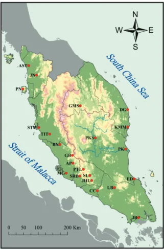
Peninsular Malaysia or West Malaysia is a part of Malaysia that is separated from East Malaysia by South China Sea (CSC). The major mountain range that forms the backbone of Peninsula is Titiwangsa Mountains, which divides Peninsular Malaysia into eastern and western parts. It also serves as a demarcation line that divides different rainfall pattern between eastern and western part of Peninsular Malaysia (Fig. 1). In general, the rainfall of Peninsula is subjected to the influence of two monsoons, which are southwest monsoon from May to September and the northeast monsoon from November to March (Liew and Fredolin 2002; 2008; Fredolin and Alui 2002). The two monsoons are separated by two inter-monsoon periods. In northeast monsoon period, the east coast of Peninsula would incur
substantial rainfall, while the southwest monsoon has less influence on rainfall over the Peninsula and off shore of SCS due to topography effect.
Fig. 1 The locations of meteorological stations used in this study
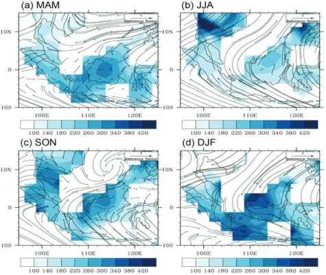
In addition, the monthly mean surface meridional and zonal wind data from 1948/1~2013/12 obtained from the NCEP Reanalysis data (National Centers for Environmental Prediction Reanalysis, retrieved from http://www.esrl.noaa.gov/psd/data/gridded/data.ncep.reanalysis. surface.html) and the monthly mean surface rainfall analyzed by GPCC (Global Precipitation Climatology Centre, retrieved from http://www.esrl.noaa.gov/psd/data/gridded/data.gpcc.html) with a spatial resolution of 2.5° longitude X 2.5° latitude during 1901/1~2012/2 for the seasonality analysis of Malaysia, are shown in Fig. 2. During the boreal autumn seasonal that transition from summer monsoon to winter monsoon, the convective centre, which is located at the adjacent bay of Begal, progresses gradually from northern to southeastern region (Chang et al. 2005). Accompanying the moving of the maximum convection is the spatial variation of rainfall in Malaysia till winter monsoon. During the boreal spring, the maximum convective which anchor at the near/south of the equator is withdrawn. The spring rainfall moves from the southern to north part of the Peninsular Malaysia.
Fig. 2 The average meridional and zonal wind (vector) and rainfall (contour) for the (a) MAM, (b) JJA, (c) SON, and (d) DJF.
Ng (2013) indicated that the rainfall patterns in Peninsular Malaysia could be divided into unimodal (annual) and bimodal (semiannual) patterns. The unimodal pattern of rainfall is shown in the East Coast Peninsula. Most rainfall is seen in the autumn (SON, Sep-Oct-Nov) and winter (DJF, Dec-Jan-Feb). The spring (MAM, Mar-Apr-May) and summer (JJA, Jun-Jul-Aug) are the dry periods. For the unimodal patterns, the rainfall in Peninsular Malaysia is primarily influenced by the northeast monsoon. On the other hand, the bimodal pattern is mainly observed in the western Peninsula. The wet seasons appear in MAM and SON and JJA and DJF are the seasons with lower rainfall amount along the western Peninsula. The characteristic bimodal pattern of rainfall is weakened from south central areas to northern Peninsula as a result of the transition between DJF and JJA and the migration of maximum convection. This has resulted in temporal-distribution variation of rainfall in Peninsular Malaysia (Ng 2013).
2. Data
The daily precipitation data from 22 automatic rainfall stations selected based on 90% data ≧ integrity in Peninsula from January 1971 to December 2007 were provided by the Department of Irrigation and Drainage Malaysia (DIDM). The geographical coordinates and the detailed descriptions of the stations are shown in Table 1, and in Fig. 1. In this study, we used the annual and seasonal maximum daily rainfall data to analyze extreme rainfall in Peninsular Malaysia. We also used the GEV
distribution of extreme rainfall to describe the occurrence probability of extreme rainfall. Besides, we have made use of the inverse distance weighted (IDW) interpolation algorithm in geographical information system software (ArcGIS) for the mapping of the geospatial distribution of extreme rainfall.
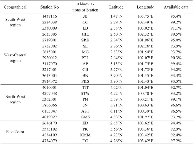
Table 1 The list of 22 rainfall stations with their geographical coordinates in this study and the percentage of their available data
Geographical Station No Abbrevia-
tions of Station Latitude Longitude Available data
1437116 JB 1.47°N 103.75°E 95.4% 2224038 CC 2.29°N 102.49°E 99.2% South-West region 2330009 LB 2.38°N 103.02°E 91.1% 2623085 JHL 2.60°N 102.32°E 99.5% 2719001 SRB 2.74°N 101.96°E 95.0% 2722002 SL 2.76°N 102.26°E 93.9% 2815001 MG 2.83°N 101.54°E 93.7% 2920012 PTL 2.94°N 102.07°E 90.3% 3117070 AP 3.13°N 101.75°E 99.4% 3217001 GB 3.27°N 101.73°E 94.2% 3613004 BN 3.70°N 101.35°E 93.4% West-Central region 3924072 PKS 3.90°N 102.43°E 93.5% 4010001 TIT 4.02°N 101.04°E 92.7% 4207048 STW 4.22°N 100.70°E 93.2% 5302001 PN 5.39°N 100.21°E 99.1% 5806066 JN 5.81°N 100.63°E 96.6% North-West region 6103047 AST 6.11°N 100.39°E 96.5% 4819027 GMS 4.88°N 101.97°E 93.7% 2636170 ED 2.65°N 103.62°E 94.4% 3533102 PK 3.56°N 103.36°E 92.9% 4234109 KMM 4.23°N 103.42°E 92.4% East Coast 4734079 DG 4.76°N 103.42°E 97.2%
Methods
1. Generalized extreme value (GEV) distribution
A series of independent observation dataXt1,Xt2,...,Xtiare blocked into groups of a regular time-scale. In this paper, i represent the number of observations blocked into a period of year, represented by t, and the maximum of the group
, ,...,
, maxMn Xt1 Xt2 Xti t1,2,...,n
where M corresponds to the annual maximum of observations. The distribution of n M can be derives n
for all values of n, hence
nn
n z Pr X z,X z,...,X z F(z)
M
when n,
F(z) nwill be a non-degenerate distribution. Following the Fisher and Tippett (1928)Theorem, If M exist sequences of constants an n > 0, bn R, Then
), ( z b M Pr H z an n n as
n
for an extreme distribution H(z) belongs to one of the three types
I : H(z) = exp z a b z , exp II : H(z) = , exp , 0 a b z ; , b z b z III : H(z) = , 1 , exp a b z , , b z b z
where a is scale parameter, b is location parameter, and is shape parameter. These three types of extreme value distributions were known as the Gumbel, Frechet, and Weibull distribution, respectively. All three types of distribution can be combined into a single function of the form which was called the Generalized Extreme Value (GEV) distribution (Jenkinson 1955).
H(z) =exp
/ 1 1 zThe parameter,,represents location parameter, scale parameter, and shape parameter respectively.
All three types of GEV were determined by shape parameter When 0, it would be a Gumbel distribution. If 0, the associated distribution is called Frechet distribution, which is known as the "fat-tail" distribution. At last, when 0, the distribution type would be a Weibull distribution.
2. Parameter estimation
The corresponding probability density functions (pdf) of GEV distribution is given by h(z) = / 1 / 1 1 1 exp 1 1 z z
and the cumulative distribution functions (cdf) of the GEV is H(z) = exp / 1 1 z
The unknown parameters ξ, σ, and μ were estimated in this study using the maximum likelihood estimator (MLE) and the L-moment estimator (LM).
(1) Maximum likelihood estimation (MLE)
In a GEV distribution, the probability density functions are written as h(zi |
,
,
), and ξ, σ,and μare the unknown parameters. The MLE is defined as
n i i 1 , , | z h ) , , ( L
The log-likelihood for the GEV parameters when 0 that the function is given by
n i n i i i z z 1 1 / 1 1 log 1 log 1 1 log n , , l
provided thatn
i
z
i,...,
2
,
1
,
0
1
(2) L-moment estimation (LM)For a real-value random variable X, the random samples are arranged in ascending order where the
n is the sample size. That is X1:nX2:n Xn:n Then the r-th LM of random variable X are defined
by (Hosking 1990)
...
2
,
1
,
0
,
1
)
1
(
: 1 0 1
EX
r
k
r
r
r r kr k k r
and the LM are thereby defined by
1 0 * 1( ) , 0,1,2,... ) (H H dH r zP
r r
where
1 log
, 0 ) (
H H z , ) ( 0 * , *
r k k k r r H p H P and
k
k
r
k
r
p
r k k r(
1
)
* ,The first four LM are
1 0 1EX
z
(
H
)
dH
1 0 2 : 1 2 : 2 2(
)(
2
1
)
2
1
dH
H
H
z
X
X
E
dH H H H z X X X E
1 0 2 3 : 1 3 : 2 3 : 3 3 ( 2 ) ( )(6 6 1) 3 1
1 0 2 3 4 : 1 4 : 2 4 : 3 4 : 4 4 ( 3 3 ) ( )(20 30 12 1) 4 1 dH H H H H z X X X X E
3. Goodness-of-fit test
In this study, we used the two-sample Kolmogorov-Smirnov (K-S) test introduced by Justel et al. (1997) to compare the sample distribution functions and the empirical distribution functions under the 0.05 confidence level to determine whether the two samples come from the same distribution. The K-S test statistic are defined as
max(F1(x)F2(x))
where theF1(x)is the sample cumulative distribution functions andF2(x)is the empirical cumulative distribution functions. The K-S test is defined by
) x ( ) x ( : 1 2 0 F F H versus H1:F1(x)F2(x)
when
H
0:
h=0, F1(x)and F2(x) are from the same distribution, on the contrary, whenH :h=1, 1) x (
1
F and F2(x) are from different distributions.
4. Return level
One of the applications of the extreme value theory is to estimate the probability of maximum rainfall event Xp, which is termed the return level, of the events occurrence in an estimated time interval
t. The estimated return level was obtained by the inverse of H(z).
1 log(1 1) t XpResults and discussion
1. The changes of temporal and spatial distribution of extreme rainfall
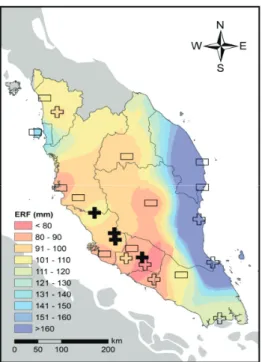
Fig. 3 shows the average annual daily maximum of rainfall for all 22 stations during 1971-2007 over the Peninsular Malaysia. The greatest rainfall recorded was at station ED, which located in the East Coast Peninsula where the average annual daily maximum rainfall is 226.0 mm day-1, while the JHL
station that situated in the Negeri Sembilan, which is located in the west central region, was the lowest. Generally, East coastal part receives the highest amount of rainfall over Peninsula. Several previous studies have indicated that the higher rainfall intensity was recorded at the same area and they have proposed that it was influenced by the northeast monsoon (Suhaila and Jemain 2012; Wan Zin et al. 2010). Besides, an increasing trend of extreme rainfall intensity was recorded in small part of the west central region, including the stations GB, BN, AP, and SL. The annual increase of the rainfall amount for these four stations is 0.6mm, 0.8mm, 0.5mm, and 1.3mm, respectively. As discussed in the previous section, we found that an increasing trend was recorded in the west central areas of Peninsula, which has low intensity of extreme rainfall in the past. This finding suggests that the west central areas will possibly face with extreme flooding in the future.
Fig. 3 The average extreme rainfall intensity from 1971 to 2007 in Peninsular Malaysia. The plus sign represents the increase trend, and the decrease trend is marked by the minus sign. Solid plus/minus indicates the statistical significance at the p≦0.1 level, and the open plus/minus represents the statistical significance at the p≧0.1 level.
Seasonally, the highest annual mean daily maximum rainfall was recorded in PN during months of MAM and JJA, which were 93.1 mm day-1 and 97.9 mm day-1, respectively. At the meantime, the
highest rainfall intensity of JHL was the lowest over Peninsula. A similar result was shown in the SON. During the SON, the largest rainfall intensity was recorded at DG stations, which located in the north east region, where the average total was 124.7 mm day-1. The maximum rainfall intensity was then
recorded at the station ED in south east areas during the DJF season and the value was marked as 214.6 mm day-1. This is most likely due to the influence of winter monsoon (Wan Zin et al. 2010). Johnson
(2005) indicated that the topography effect, which happens when northeast monsoon travels towards coastal mountain ranges in Vietnam, Malaysia and the east coast of the Philippines, has resulted in a maximum rainfall in Peninsular Malaysia during the DJF. Furthermore, the cold surge vortices from the Philippine area and Borneo have also contributed in bringing a maximum rainfall in Peninsular Malaysia (Chen et al. 2013). In general, During SON and DJF, the extreme rainfall intensity in the western Peninsula was recorded with a lower value, particularly in DJF.
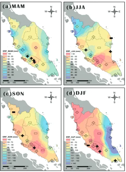
Fig. 4 shows the seasonal variability of the extreme rainfall intensity during 1971-2007. An increasing trend was found in the west central areas during the MAM (Fig. 4a) and SON (Fig. 4c) seasons. There are four (JHL, AP, PTL, SL) and two ( BN, JHL) stations’ values achieving statistically significant level (p≦0.1) during MAM and SON, respectively. On the other hand, a statistically
significant decreasing trend was observed in JN, which is located at northern areas during SON. During DJF (Fig. 4d), the stations SL, CC, and JB in southern region of Peninsula were recorded with an increasing trend of extreme rainfall. Nonetheless, the MG station had showed a statistically significant reversed trend. Lastly, there was no obvious different in the spatial pattern of extreme rainfall during JJA seasons (Fig. 4b).
Fig. 4 The trend and average extreme rainfall intensity from 1971 to 2007 in Peninsular Malaysia during the (a) MAM, (b) JJA, (c) SON, and (d) DJF. The plus sign represents the increase trend, and the decrease trend is marked by the minus sign. Solid plus/minus indicates the statistical significance at the p 0.1 level, and the open plus/minus represents the statistical significance ≦ at the p 0.1 level.≧
2. Generalized extreme value (GEV) distribution
(1) Estimates parameters of the GEV distributionIn this study, both MLE and LM parameter estimations were used to derive the GEV distribution on the annual and seasonal maximum rainfall. In addition, the two sample K-S test was used to serve as a fit test to compare the sample distribution function and the empirical distribution function from different parameter estimations
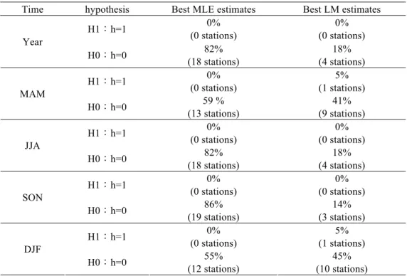
Based on the result of K-S test (Table 2), all of the stations failed to reject null hypothesis under 0.05 confidence level except the station of ED in MAM months and BN in DJF seasons under the method of LM estimation. Based on the Kolmogorov-Smirnov statistic value, the MLE was identified as the best fitness estimation method for the GEV distribution during the 1971-2008 periods. Approximately 82% of the total stations achieved the best fitness parameter estimation based on the MLE. Furthermore, a similar finding was found in JJA and SON seasons, in which approximately 82% and 86% of the total stations achieved best fitness parameter estimation, respectively. For the MAM and DJF months, the best MLE estimate was found in 59% of the total stations in MAM and 55% of the total stations in DJF; while the best LM estimate was found in 41% and 45% of the total stations in MAM and DJF, respectively. A similar result was shown in Fig. 5 based on a different goodness-of-fit test, the Q-Q plot. As mentioned previously, in general, the MLE method of parameter estimation gave more reliable result than the LM method for GEV distribution in this study.
Table 2 The comparison of the results of MLE and LM estimators in this study. When H1:h=1, null
hypothesis rejected; when H0:h=0, null hypothesis failed to be rejected.
Time hypothesis Best MLE estimates Best LM estimates
H1:h=1 0% (0 stations) 0% (0 stations) Year H0:h=0 82% (18 stations) 18% (4 stations) H1:h=1 0% (0 stations) 5% (1 stations) MAM H0:h=0 59 % (13 stations) 41% (9 stations) H1:h=1 0% (0 stations) 0% (0 stations) JJA H0:h=0 82% (18 stations) 18% (4 stations) H1:h=1 0% (0 stations) 0% (0 stations) SON H0:h=0 86% (19 stations) 14% (3 stations) H1:h=1 0% (0 stations) 5% (1 stations) DJF H0:h=0 55% (12 stations) 45% (10 stations)
Fig. 5 The Q-Q plot of the observed value and the GEV distribution theoretical value of MLE and LM estimations for 22 stations in Peninsular Malaysia during the annual and seasonal times.
(2) Return period estimates
The best fitness parameter estimation was used to estimate the return levels of the extreme rainfall for the return periods of 50-year and 100-year. According to the return level estimate, the extreme rainfall was greater in the 50-year return level in the majority of the stations of Peninsular Malaysia during 1971-2007. Further, six stations, the AST, STW, TIT, GB, MG, and JB stations, which are located in the west Peninsular Malaysia, was recorded to have a higher than 100-year return level estimates. Seasonally, the rainfall stations with extreme rainfall during the JJA months that had more than 100-year return level were found in the west region except for the DG station. For DJF, more than half of the stations were experiencing 100-year return level estimates. Moreover, the extreme rainfall events that were higher than a 100-year return level were recorded in approximately 32% and 36% of the total stations during the MAM and SON seasons, respectively.
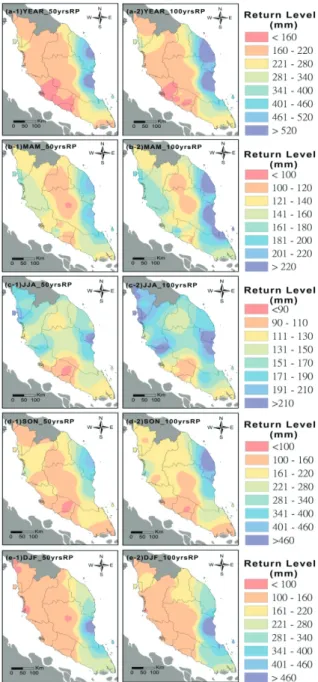
Shown in the Fig. 6a, is the spatial variation of annual extreme rainfall intensity under 50-year and 100-year return periods. The eastern part of Peninsular Malaysia was found to have a maximum rainfall with more than 600 mm day-1 in the 50-year return period and was higher than 700 mm day-1 under
100-year return period. The maximum rainfall values were found to be gradually decreased from the eastern area to the west central part. A lower than 160 mm day-1 of maximum rainfall was found at the
west central part of Peninsular Malaysia under 50-year and 100-year return periods.
Seasonally, a higher than 200 mm day-1 and 250 mm day-1 of maximum rainfall values were found
in eastern part under 50-year and 100-year return periods, respectively. On the other hand, the areas that received lower than 130 mm day-1 of extreme rainfall values were located in inland and southwest
coastal areas during the MAM months (Fig. 6b). In JJA (Fig. 6c), for the 50-year return period, we found a maximum estimate values of > 220 mm day-1 and it increased to 270 mm day-1 at 100-year
return period in southeast part. Secondly, the northwest part of Peninsular Malaysia was recorded to have extreme rainfall events between 131-190 mm day-1 at 50-year return period and it increased to 220
mm day-1 under 100-year return period. As shown in Fig. 6d, the eastern part of Peninsular Malaysia
was recorded to have the highest rainfall value of >400 mm day-1 and a large station of southwest area
was found with a minimum value of <140 mm day-1 at 50-year return period in SON. For the 100-year
return period, the maximum rainfall was recorded to be 560 mm day-1 in eastern region and the southwest part, and these regions have showed little change of the maximum rainfall values during the autumn season. For DJF, as shown in Fig. 6e, the maximum rainfall with more than 480 mm day-1 was recorded in the southeast region at 50-year return period and >600 mm day-1 at 100-year return period.
In the meantime, the minimum rainfall of 80-200 mm day-1 was found in other regions of Peninsular
Malaysia either at 50-year or at 100-year return period.
In general, the return level estimate of extreme rainfall between the western and eastern parts of Peninsular Malaysia was evidently different. The scale variations of the return level registered in the eastern part were greater than that of the western region, particularly during the SON and the DJF seasons. In the other hands, the observed rainfall record in the western part had readily exceeded the
100-year return level estimation. These results showed that we might have difficulties in estimating the extreme rainfall event in the western part of Peninsular Malaysia through the GEV distribution model. This has suggested a limitation on the use of GEV distribution, although it has been a best method in goodness-of-fit test. In another point of view, the results might also imply that there was a shift of spatial distribution of the tendency of extreme rainfall in recent years.
Fig. 6 The spatial variation of the annual and seasonal extreme rainfall intensity under 50-year and 100-year return periods.
Summary and conclusions
In this study, we have analyzed the extreme rainfall events in Peninsular Malaysia based on data collected from a total of 22 rainfall stations provided by the Department of Irrigation and Drainage Malaysia from the period of 1971-2007. The annual and seasonal daily maximum rainfall values were applied in the extreme rainfall analysis. The GEV distribution of the extreme rainfall was used to calculate the return value. For the parameter estimations, the MLE and LM estimations were used to derive the GEV distribution. MLE is suggested to be the best estimation in this study based on the result of K-S test and Q-Q plot.
In general, the highest extreme rainfall intensity was recorded in the eastern part of Peninsula during 1971-2007, while the lowest extreme rainfall intensity was found in west central areas. Besides, our study suggests that there is a positive trend of extreme rainfall intensity at west central region in recent year. These results would contribute to the prediction of extreme flooding events in the future. Seasonally, the highest amount of rainfall was recorded at PN in northern part during MAM and JJA. While, during the SON and DJF, the highest rainfall amount was recorded at the stations DG and ED, respectively. However, the lowest extreme rainfall intensity across different seasons, except DJF, was documented in JHL. Based on the results from seasonal analysis, we suggest that there is a possibility of flood disaster affecting the west central areas during the MAM and SON, while the northern part of Peninsula will probably suffered from the drought during SON.
The best fitness parameter estimation was used in this study to estimate the return levels for the return periods of 50-year and 100-year. We are aware that there is an apparent difference between the western and eastern part of Peninsular Malaysia in terms of the scale variations of the return level, in which the eastern part was greater than the western region. In the other hand, the observed rainfall level in the western region had readily exceeded the 100-year return level estimation. Our results highlight a limitation on the use of GEV distribution to estimate the return levels of extreme rainfall in the western part of Peninsular Malaysia, although it seems to be the best method from the goodness-of-fit test. Based on the result of the extreme rainfall tendency, it is suggested that there is a shift of spatial distribution of extreme rainfall tendency in recent years.
Acknowledgment
The authors wish to thank Dr. Liew Juneng of the Universiti Kebangsaan Malaysia (UKM) and Mesoscale and Orographic Precipitation Laboratory lead by Prof. Cheng-Ku Yu to make this study possible. We are grateful to the Department of Irrigation and Drainage Malaysia (DIDM) for providing the rainfall data. The authors would also like to thank two anonymous reviewers for their suggestions that led to the improvement of this manuscript.
References
Aryal, Santosh K., Bates, Bryson C., Campbell, Edward P., Li, Yun, Palmer, Mark J., and Viney, Neil R. (2009): Characterizing and modeling temporal and spatial trends in rainfall extremes, Journal of
Hydrometeorology, 10:241-253.
Azpurua, Marco and Dos Ramos, Karina (2010): A comparison of spatial interpolation methods for estimation of average electromagnetic field magnitude, Progress In Electromagnetics Research M, 14:135-145.
Beirlant, Jan, Vynckier, Petra, and Teugels, Jozef L. (1996): Excess functions and estimation of the extreme-value index, Bernoulli, 2(4):293-318.
Chang, Chih-Pei, Wang, Zhuo, McBride, John, and Liu, Ching-Hwang (2005): Annual cycle of Southeast Asia—maritime continent rainfall and the asymmetric monsoon transition, Journal of
Climate, 18:287-301.
Chen, Tsing-Chang, Tsay, Jenq-Dar, Yen, Ming-Cheng, and Matsumoto, Jun (2013): The winter rainfall of Malaysia, Journal of Climate, 26:936-958.
Chu, Pao-Shin, Zhao, Xin, Ruan, Ying, and Grubbs, Melodie (2009): Extreme rainfall events in the Hawaiian Islands, Journal of Applied Meteorology and Climatology, 48:502-516,
Coles, Stuart and Pericchi, Luis R. (2003): Anticipating catastrophes through extreme value modelling,
Applied Statistics, 52:405-416.
Coles, Stuart, Pericchi, Luis R., and Sisson, Scott (2003): A fully probabilistic approach to extreme rainfall modelling, Journal of Hydrology, 273:35-50.
Fredolin, T. Tangang and Alui, Bahari (2002): Enso influences on precipitation and air temperature variability in Malaysia. Proceedings of the Regional Symposium on Environment and Natural
Resources, April 10-11, Kuala Lumpur, 1:124-131.
Hershfiels, David M. (1973): On the probability of extreme rainfall events, Bulletin American
Meteorological Society, 54(10):1013-1018.
Hosking, J. R. M. (1990): L-moments: analysis and estimation of distributions using linear combinations of order statistics, Journal of the Royal Statistical Society B, 52:105-124.
Hosking, J. R. M., Wallis, James R., and Wood, Eric. F. (1985): Estimation of the generalised extreme value distribution by the method of probability-weighted moments, Technometrics, 27:251-261. Intergovernmental Panel on Climate Change, IPCC. (2007): Observed changes in climate and their
effects. Climate change 2007: Synthesis Report.
http://www.ipcc.ch/publications_and_data/publications_ipcc_fourth_assessment_report_synthe sis_report.htm (last accessed 18 September 2012).
Jenkinson, A. F. (1955) : The frequency distribution of the annual maximum (or minimum) values of meteorological elements, Quarterly Journal of the Royal Meteorological Society, 81(348):158-171. Johnson, Richard H. (2005): Mesoscale processes, in B. Wang, (Ed.) The Asian Monsoon. UK: Springer.
Juneng, Liew, Tangang, Fredonlin. T., and Reason, Chris J. C. (2007): Numerical case study of an extreme rainfall event during 9-11 December 2004 over the east coast of Peninsular Malaysia,
Meteorology and Atmospheric Physics, 98:81-98.
Juneng, Liew, Tangang, Fredonlin T., Kang, Hongwen, Lee, Woo-Jin, and Yap, Kok Seng (2010): Statistical downscaling forecasts for winter monsoon precipitation in Malaysia using multimodel output variables, Journal of Climate, 23:17-27.
Justel, Ana, Peña, Daniel, & Zamar, Rubén (1997): A multivariate Kolmogorov-Smirnov test of goodness of fit, Statistics & Probability Letters, 35:251-259.
Kottek, Markus, Griesek, Jürgen, Beck, Christoph, Rudolf, Bruno, and Rubel, Franz (2006): World map of the K ppen-Geiger climate classification updated, Meteorologische Zeitschrift, 15(3):259-263. Koutsoyiannis, Demetris (2004): Statistics of extremes and estimation of extreme rainfall: Ⅰ.
Theoretical investigation, Hydrological Sciences Journal, 49(4):575-590.
Koutsoyiannis, Demetris, and Baloutsos, George (2000): Analysis of a long record of annual maximum rainfall in Athens, Greece, and design rainfall inferences, Natural Hazards, 29:29-48.
Lavenda, Bernard H. and Cipollone, Elvio (2000): Extreme value statistics and thermodynamics of earthquakes: aftershock sequences, Annali Di Geofisica, 43(5):967-982.
Liew, Juneng and Fredolin, T. Tangang (2002): Malaysia northeast monsoon precipitation variability and its relationships with tropical sea level pressure, Proceedings of the Regional Symposium on
Environment and Natural Resources, April 10-11, Kuala Lumpur, 1:251-260.
Liew, Juneng and Fredolin, T. Tangang (2008): Level and source of predictability of seasonal rainfall anomalies in Malaysia using canonical correlation analysis, International Journal of Climatology, 28:1255-1267.
Madsen, Henrik, Rasmussen, Peter F., and Rosbjerg, Dan (1997): Comparison of annual maximum series and partial duration series methods for modeling extreme hydrologic events, 1, At-site modeling, Water Resources Research,33(4):747–758.
Martins, Eduardo S. and Stedinger, Jery R. (2000): Generalized maximum-likelihood generalized extreme-value quantile estimators for hydrologic data, Water Resources Research, 36(3):737-744. McNeil, Alexander J. and Frey, Rüdiger (2000): Estimation of tail-related risk measures for
heteroscedastic financial time series: an extreme value approach, Journal of Empirical Finance, 7:271-300.
Nadarajah, Saralees and Choi, Dongseok (2007): Maximum daily rainfall in South Korea, Journal of
Earth System Science, 116(4):311-320.
Ng, Yuen Yi (2013): An analysis of rainfall periodicity of maritime continent: a case study in Peninsular Malaysia (1971-2007), Journal of Geographical Science, 71: 93-111. (in chinese)
Nieuwolt, Simon (1968): Diurnal rainfall variation on Malaya, Annals of the Association of American
Geographers, 58(2):313-326.
Uncertainties and trends in extreme rainfall series in Tuscany, Italy: effects on urban drainage networks design, Water Science and Technology, 37(11):195-202.
Parida, Bhagabat P. (1999): Modelling of Indian summer monsoon rainfall using a four-parameter Kappa distribution, International Journal of Climatology, 19:1389-1398.
Park, Jeong-Soo and Jung, Hyun-Sook (2002): Modelling Korean extreme rainfall using a Kappa distribution and maximum likelihood estimate, Theoretical and Applied Climatology, 72:55-64. Park, Jeong-Soo, Jung, Hyun-Sook, Kim, Rae-Seon, and Oh, Jai-Ho (2001): Modelling summer extreme
rainfall over the Korean peninsula using Wakeby distribution, International Journal of
Climatology, 21:1371-1384.
Raynal-Villasenor, Jose A. (2012): Maximum likelihood parameter estimators for the two populations GEV distribution, International Journal of Research & Reviews in Applied Sciences, 11(3):350-357.
Sobey, Rodney J. (2005): Extreme low and high water levels, Coastal Engineering, 52:63-77.
Sugahara, Shigetoshi, da Rocha, Rosmeri P., and Silveira, Reinaldo (2009): Non-stationary frequency analysis of extreme daily rainfall in Sao Paulo, Brazil, International Journal of Climatology, 29:1339-1349.
Suhaila, Jamaludin and Jemain, Abdul Aziz (2007): Fitting daily rainfall amount in Malaysia using the normal transform distribution, Journal of Applied Sciences, 7(14):1880-1886.
Suhaila, Jamaludin and Jemain, Abdul Aziz (2012): Spatial analysis of daily rainfall intensity and concentration index in Peninsular Malaysia, Theoretical and Applied Climatology, 108:235-245. Suhaila, Jamaludin, Deni, Sayang Mohd, Wan Zin, Wan Zawiah, and Jemain, Abdul Aziz (2010): Spatial
patterns and trend of daily rainfall regime in Peninsular Malaysia during the southwest and northeast monsoons: 1975-2004, Meteorology and Atmospheric Physics, 110:1-18.
Wan Zin, Wan Zawiah, Jamaludin, Suhaila, Deni, Sayang Mohd, and Jemain, Abdul Aziz (2010): Recent changes in extreme rainfall events in Peninsular Malaysia: 1971-2005, Theoretical and Applied
Climatology, 99:303-314.
Wan Zin, Wan Zawiah and Jemain, Abdul Aziz (2010): Statistical distribution of extreme dry spell in Peninsular Malaysia, Theoretical and Applied Climatology, 102:253-264.
Wan Zin, Wan Zawiah, Jemain, Abdul Aziz, and Ibrahim, Kamarulzaman (2009): The best fitting distribution of annual maximum rainfall in Peninsular Malaysia based on methods of LQ-moment,
Theoretical and Applied Climatology, 96:337-344.
Wilks, Daniel S. (1993): Comparison of three-parameter probability distribution for representing annual extreme and partial duration precipitation series, Water Resources Researces, 29:3543-3549. Zakaria, Zahrahtul Amani, Shabri, Ani, and Ahmad, Ummi Nadiah (2012): Regional frequency analysis
of extreme rainfalls in the west coast of Peninsular Malaysia using partial L-moments, Water
Resour Manage, 26:4417-4433.
(2002a): Selecting a probability distribution for extreme rainfall series in Malaysia, Water Science
& Technology, 45(2):63-68.
Zalina, Mohd Daud, Kassim, Amir Hashim Mohd, Desa, Mohd Nor Mohd, and Nguyen, Van-Thanh-Van (2002b): Statistical analysis of at-site extreme rainfall processes in Peninsular Malaysia, in H. A. J., Van Lanen, & S., Demuth (Eds.), FRIEND 2002: Regional Hydrology: Bridging the Gap between
Research and Practice (pp. 61-68). Wallingford: IAHS.
Zhao, Er-Xu, Lu, Jun-Mei, and Ju, Jian-Hua (2006): Impacts of onset of summer monsoon over Southeast Asia on the rainy season in Yunnan, Journal of Tropical Meteorology, 22(3):209-216. (in chinese)
Zwiers, Francis W., Zhang, Xuebin, and Feng, Yang (2011): Anthropogenic influence on long return period daily temperature extremes at regional scales, Journal of Climate, 24:881-892.
投稿日期:104 年 09 月 14 日 修正日期:104 年 10 月 10 日 接受日期:104 年 10 月 10 日