2012 South-East Asian Conference on Business & Management Technology and Education 2012 年 7 月 17 日
Continual equipment investment is the only option for all global
semiconductor manufacturers?
Ching-Wen Mo
1Tsangyao Chang
21
Department of Finance, Meiho, Pingtung University, Taiwan
x00002212@meiho.edu.tw
2
Department of Finance, Feng Chia University, Taichung, Taiwan
x00005038@meiho.edu.tw
Abstract
In this paper, we focus on the semiconductor manufacturing industry and investigate whether the firms’ sales growth and their Return on Equity (ROE) have an asymmetric nonlinear relationship in different debt ratio regimes by using financial statement-based data and employing a more powerful panel threshold regression model developed by Hansen (1999) over the 1999 first quarter (1Q) to 2005 third quarter (3Q) period. The result shows that there exists a double threshold effect and that the threshold values of debt ratio are
ˆ
1
0.4935 and
2
ˆ
0.6847
. When the debt ratio is below 68.47%, ROE will be increased by continual equipment investment. However, when the debt ratio is above 68.47%, ROE will be decreased by continual equipment investment. These findings could be valuable for both the market investors to search their target of investment and corporation managers who can utilize them to adjust their production strategy and investment decision for increasing their business per formance.Keywords: Panel-unit root test; Panel threshold regression model;
I. INTRODUCTION
In the past few decades, the Information Technology industry has experienced the most rapid growth among all industries worldwide, with semiconductor manufacturers having played an arguably crucial role in the supply chain.
In the field of semiconductor wafer manufacturing alone, the innovative technologies of the manufacturing process and the enlargement of wafer size are two main motive powers that contributed to the industry’s continued growth. The semiconductor manufacturing industry is a typical oligopolistic industry that has capital and technical thresholds. In order to maintain the entry barrier and decrease production costs, semiconductor manufacturers often propose new investment plans, among which is enlarging the wafer size. 1 However, firms need considerable funds to support these plans. In practice, limited internal capital compels financial managers to adopt external financing for fund-raising. These investment plans, which are intended to fill enormous funds demands, must gain the unanimous approval of both the shareholders and debt-holders. Furthermore, financial managers must propose powerful financial prospects to acquire their accommodators’ financial assistance.
In this paper, we collect 23 listed multi-national semiconductor manufacturers and focus on the firms’ output aspect. We used the sales revenue data contained in their financial report to measure the firms’ output level. We attempt to utilize the firms’ sales growth rate as the proxy for the variation of a semiconductor manufacturer’s products. However, the firm’s sales revenue is the product of price by quantity thus, factors that influence increase in a firm’s sales revenue is either a raise in price or an
1
The building cost of 8-inch wafer fab and 12-inch wafer fab needs $1 billon and $3 billons, respectively.
increase in production. According to Moore’s Law, the complexity and efficiency of IC chip will increase to twice its current capacity while its price will decrease by half every 18 months. Furthermore, Gordon (2000) points out that the decreasing rate of price change in computer hardware (including peripherals) were at an average rate of -14.7 percent between 1987 and 1995 and -31.2 percent between 1996 and 1999. In addition, Oliner et al. (2003) show that the relative inflation rate2 in semiconductor sector were at an average rate of -28.9 percent between 1974 and 1990, -21.8 percent between 1991 and 1995 and -44.7 percent between 1996 and 2001. Hence, the price of computer hardware appeared to have a tendency of accelerating depreciation after 1995. To be brief, the price of semiconductor may rise temporarily in the short run, but it will drop in the long run.
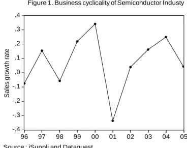
Consequently, increasing production is the only way firms to raise sales revenue drastically. For this reason, the firm’s production strategy is either to enlarge wafer size or accelerate innovative technologies of manufacturing process. However, both strategies require considerable funds to be carried out. We consider both strategies as continual equipment investment. As stated earlier, due to the limited internal fund supply, it becomes necessary for firms to seek external financing. Figure 1 illustrates the growth rate of the semiconductor industry in total sales; from here we can see that there is no question as to whether there have been striking variations in total demand, many of which have been unanticipated. Since the semiconductor manufacturers face an extremely fluctuating market demand and because the characteristics of higher capital threshold exist in the semiconductor manufacturing industry, they will require external financing to meet the demands for huge funds. The question then becomes whether there exists other options for semiconductor manufacturers or is it limited to continual equipment investment.
2
The relative inflation rate is output price inflation in
Semiconductor sector minus that in the “other final-output” sector (for further details, see Oliner et al., 2003).
Modigliani and Miller (1958, 1963) published seminal papers on the capital structure, weighted average cost of capital, and corporate valuation. The major difference between the assumptions of these two seminal papers is that the former assumed no taxes and the latter considered corporate income tax deductibility of interest (tax shields effect). Miller (1977) modified this assumption by introducing personal taxes as well as corporate taxes into the gain-to-leverage model. Jensen and Meckling (1976) utilized agency costs to discuss the conflict between principals and agents. They suggested that there is an optimum ratio of debt to equity that will be chosen because it minimizes total agency costs. Consequently, the optimal capital structure can result in a trade-off between the tax shields benefit of debt and agency costs. Castanias (1983) argued that if managers increase financial leverage then the possibility of bankruptcy also increases and the probability of bankruptcy has a negative effect on the firm’s value. Therefore, the optimal ratio of debt to equity is determined by a trade-off between interest tax shields and bankruptcy costs. Leland (1994) and Leland and Toft (1996) modeled corporate valuation by assuming that the present value of business disruption costs and the present value of lost interest tax shields are affected by different capital structures of firm. The result is similar, an optimal capital structure as a trade-off between the tax deductibility of interest expenses and business disruption costs.
By combining the above arguments with the trade-off model, we predict that a few semiconductor manufacturers who will face an extremely fluctuating market demand will naturally need large external financing. In the future, if these firms encounter economic recession, they may incur huge losses have higher debt ratios. However, in general, most debt-holders will be reluctant to lend money to debt-heavy firms; hence, there will be an increase in financing difficulty and capital cost of firms who have higher debt ratios.
Financial ratios are widely employed as explanatory variables in the field of empirical finance to explain the
2012 South-East Asian Conference on Business & Management Technology and Education 2012 年 7 月 17 日 investment decisions of firms (Barnes (1987); Beatty
(1993); and Cleary (1999) among others). Additionally, numerous empirical researchers have utilized ROE as an indicator or proxy variable to evaluate corporate business performance or firm value (e.g. see Mramor and Mramor Kosta, 1997;Pahor and Mramor, 2001;Easton, 2004; and Nieh et al., 2008 among others). In this paper, we utilize some financial ratios to explain the business performance (ROE) of firms. These ratios include sales growth rate, debt ratio and total asset turnover rate.
In recent years, Hansen’s panel threshold regression model has been widely employed in the field of empirical finance to explore corporate investment and financing constraints (e.g. see Chen, 2003; Nieh and You, 2005; Shen and Wang, 2005; Yeh et al., 2007; and Nieh et al., 2008 among others). The purpose of this paper is to focus on the semiconductor manufacturing industry and investigate whether the sales growth and ROE of firms in the industry have asymmetric nonlinear relationship in different debt ratio regimes. We presume that the semiconductor manufacturing industry has different debt ratio thresholds that will allow for the division of all of the firms into groups, making the firms’ sales growth rate and their ROE exist asymmetric nonlinear relationship in the different debt ratio regimes. When the sales growth rate and ROE have significant positive relationship in one regime, this implies that continual equipment investment could improve a firm’s business performance. On the contrary, when they have significant negative relationship in another regime, this implies that continual equipment investment will damage a firm’s business performance. Furthermore, when the sales growth rate and ROE have an insignificant relationship in one regime, this implies that continual equipment investment might not guarantee the improvement of a firm’s business performance.
The remainder of this paper is structured as follows. Section II presents a description of the data we use. Section III describes the methodology we employ and discusses the
empirical results. It also points out some policy implications. Finally, Section IV concludes the paper.
II. DATA
In this paper, we collect data from 1999 1Q to 2005 3Q for 23 listed multi-national firms operating primarily in the semiconductor manufacturing industry. We collect these data from COMPUSTAT and the Taiwan Economic
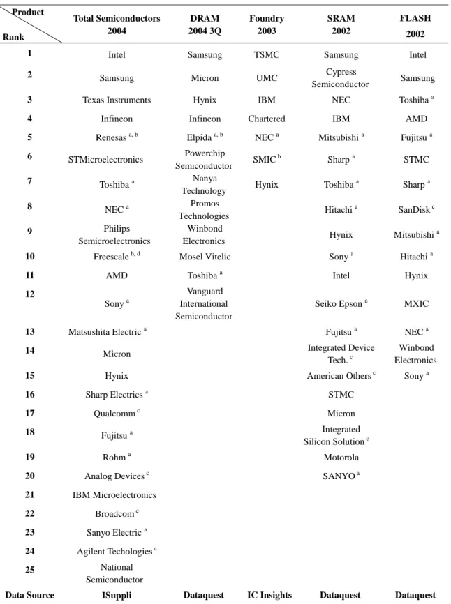
Journal (henceforth TEJ)3 database. We select our sample data from certain semiconductor market research institutions (including iSuppli Corp., IC insights Corp. and Gartner Dataquest Corp.), which provide the rankings of the top 25 semiconductor market shares worldwide in the DRAM industry (the top 12), and the Foundry industry (the top 7). This information is summarized in Table 1. We exclude Japanese companies4 that started trading publicly after 19995 and IC design houses (Fabless)6. Our empirical analysis utilize three financial ratios to explain a firm’s business performance (ROE), which are sales growth rate, debt ratio, and total asset turnover rate. Table 2 reports the summary statistics of the four financial ratios. As shown in Table 2, the Jarque-Bera test results show that the
3
The COMPUSTAT database provides quarterly data for NYSE- and NASDAQ-listed companies but only provides annual data for Korea and Taiwan listed companies. The TEJ database presents quarterly data for Korea and Taiwan listed companies.
4
We exclude Japanese semiconductor firms largely because most (NEC, Hitachi, Toshiba, Mitsubishi, among others) have split off their semiconductor manufacturing operations and jointly set up new companies with other firms in recent years. These new companies have been listed since 1999. Furthermore, these Japanese firms tend to be made up of financial groups making it difficult to distinguish semiconductor divisions from others.
5
Freescale Semiconductor and Renesas Technology, which were both listed after 1999, are good examples. Motorola split off its semiconductor manufacturing division and in 2004 set up a new company, Freescale. Mitsubishi and Hitachi split off their semiconductor manufacturing divisions and in 2002 merged them to form a new separate legal entity, Renesas.
6
Fab and Fabless companies are extremely different in terms of the structure of their assets; while Fab companies belong to the manufacturing industry, Fabless companies engage in the design, development, and marketing of their chips and adopt outsourcing strategies to have these chips manufactured.
distribution of all financial ratios approximate non-normal.
III. METHODOLOGY AND EMPIRICAL RESULTS A. Hansen Panel Threshold Autoregressive Model 3.1 Panel Unit Root models
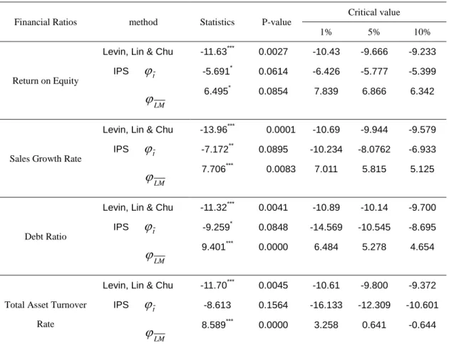
According to the trade-off theory of capital structure, the optimal ratio of debt to equity is determined by a trade-off between the interest tax shields and leverage related costs. Therefore, this paper presumes that there is a feasible debt ratio regime in the semiconductor manufacturing industry. We employ the panel threshold regression model developed by Hansen (1999) to estimate this regime and explore the asymmetric nonlinear relationship between the firms’ sales growth and their ROE in different debt ratio regimes. The results should help corporation managers adjust the firms’ capital structure or change their production strategies. From a methodological point of view, if we apply Hansen’s panel threshold regression model, we should first use panel unit root tests to verify that all financial ratio series are stationary series in order to avoid the so-called spurious regression7. Thus, we first apply several panel-based unit root tests and examine the null of a unit root in four financial ratios of our sample firms. To avoid small-sample biases, we calculate the critical values based on Monte Carlo simulations, performing 10,000 times for each test. These results are given in Table 3. We find that both the Levin-Lin-Chu (Levin et al., 2002) and Im-Pesaran-Shin (Im et al., 2003) panel-based unit root tests reject the null of non-stationarity for these ratios and indicate that they are stationary.
3.2 Threshold Autoregressive model
The results of the panel unit root test of each variable confirm that all series are stationary. We thus
7
Granger and Newbold (1974) argued that spurious regression is the estimation of the relationship among non-stationary series is without difficulty of getting higher R2 and t statistics.
perform Hansen’s panel threshold regression model and hypothesize that the firms’ sales growth rate and their ROE exist asymmetric nonlinear relationship in different debt ratio levels. Since Tong (1978) proposed the threshold autoregressive model, the utilization of this nonlinear time series model has been widely used in economic and financial research.
In estimating the threshold autoregressive model, a test to determine whether or not there are threshold effects must first be conducted. If the null cannot be rejected, then the threshold effect does not exist. To avoid the “Davies problem8”, Hansen (1999) recommended a bootstrap method to simulate the asymptotic distribution of the likelihood ratio test and compute the critical values in order to test the significance of threshold effect. Furthermore, when the null cannot be accepted, which means the threshold effect does exist, Chan (1993) demonstrated strong evidence that the OLS estimation of the threshold is super-consistent and that it can derive the asymptotic distribution. Hansen (1999) proposed a simulation likelihood ratio test to derive the asymptotic distribution when testing for a threshold and he applied the two-stage OLS method to estimate the panel threshold model. The steps are as follows. First, for any given threshold value (
), the sum of square errors (SSE) is computed separately. Second, the threshold estimator (
) is estimated by minimizing SSE. In this paper, we employ this two-stageOLS method to estimate
and then utilize
to estimate the coefficients of every regime then analyze the results.3.3 The Threshold Regression Model Construction
A Single Threshold Model can be set up as follows.
' 1
(
)
2(
)
it i it it it it it ity
X
s I d
s I d
(1)8
“Davies’ Problem” exists when the testing statistics follow a non-standard distribution because of the presence of nuisance parameters (Davies, 1977, 1987).
2012 South-East Asian Conference on Business & Management Technology and Education 2012 年 7 月 17 日
1,
2
,
' 1, 1 it it it X d a Where
y
itrepresents firms’ ROE;I
( )
is the indicator function;d
it , debt ratio, which is also the threshold variable, and
is the specific estimated threshold value;it
s
, sales growth rate;
i, the fixed effect, represents the heterogeneity of firms under different operating conditions;it
, the disturbance term, is assumed~(0,
2)
iid it
;i
represents different firms and
1 i
n
;t
represents different time periods and1 t
T
. There are two control variables (X
it) that they may influence the firm’s ROE, which ared
it: debt ratio,a
it: total asset turnover rate.Equation (1) can be written as:
' ' it i it it ity
X
sd
' ',
( )
it it i it itX
y
sd
it
it
it it its I d
sd
s I d
' it i it ity
k
,
(2) where
1,
2
,
',
'
,k
it
X
it',
sd
it'(
)
' The observations are separated into two groups dependent on whether the threshold variabled
itis larger or smaller than threshold value
. We can acquire the different regression slope estimators,
1and
2 from two different regimes and apply giveny
itandsd
itto estimatethese parameters that include
, ,
and
2.
3.4 Estimation
' ' i i i i iy
u
X
sd
, (3) where 1 1 i it t y y T
, 1 1 ( ) ( ) i it t sd sd T
, 11
i it tX
X
T
and
1 1 t it i T Taking the difference between (2) and (3)
* ' * ' * * it it it ity
X
sd
, (4) wherey
it*
y
it
y
i , *( )
( )
i( )
it itsd
sd
sd
, * it it iX
X
X
and
it*
it
i(4) is a regression that removed the individual-specific means.
Next the stacked data and errors for an individual firm, with one time period deleted.
* 2 * * i i iT
y
y
y
, * 2 * *( )
( )
( )
i i iTsd
sd
sd
, * 2 * * i i iTX
X
X
,
* * 2 * iT i i
* 1 * * * i ny
Y
y
y
,
* 1 * * * D i nsd
S
sd
sd
, * 1 * * * i nX
X
X
X
, * 1 * * * i n
,Using these notations, (4) is equivalent to
* ' * * *
D
Y
X
S
, (5) The equation (5) represents the major estimation model of threshold effect. The panel threshold regression model use two-stage OLS method. On the first stage, for any given
, the slop coefficient
can be estimated by OLS. That is,
* *
1 * *ˆ
( )
( )
( )
D D D
S
S
S
Y
(6) The vector of regression residuals is
* * ' *ˆ
*ˆ
( )
( )
DY
X
S
(7) and the sum of squared errors, SSE is * *
'
1 * * * * * * 1 D D D D SSE Y I S S S S Y (8)Chan (1993) and Hansen (1999) recommend estimation of
by least squares method and achieve by minimization of the concentrated sum of squared errors (9). Hence the least squares estimators of
is
min 1
arg
ˆ SSE
(9)
Once
ˆ
is obtained, the slope coefficient estimation is
ˆ
ˆ ˆ
. The residual vector isˆ
*ˆ ( )
*
, and the estimator of residual variance is2 2 *' * 1 1 ˆ ˆ 1 ˆ ˆ ˆ ˆ ˆ ˆ ( ) ( ) ( ) ( ) ( 1) ( 1)SSE n T n T (10)
where n represents the number of sample, T represents the periods of sample.
3.5 Testing for a Threshold
This paper hypothesizes that there exists the threshold effect of the debt ratio between the firm’s sales growth and ROE. It is important to detect whether the threshold effect is statistically significant. The null and alternative hypothesis can be represented as follows:
2 1 1 2 1 0 : :
H HWhen the null is rejected, the coefficient
1
2 the threshold effect of the debt ratio exists between the firms’ sales growth and their ROE. Alternatively, when the null is accepted, the coefficient
1
2 the threshold effect of the debt ratio doesn’t exist.Under the null hypothesis of no threshold, the model is
' '
it i it it it
y
X
sd
(11) After the fixed-effect transformation is made, we can obtain
* ' * ' * *
1 D it
G
X
S
(12) By OLS method estimate (12) that can yield the estimator1 ~
, residuals
it* and the sum of squareerrors *' *
0
SSE .
Hansen (1996) suggests that we utilize the F test
approach to determine the existence of threshold effect, and use the sup-Wald statistic to test the null.
F
F
sup
(13)
0
1
0 1
2 1 ˆ ˆ ( ) /1 ˆ / ( 1) ˆSSE SSE SSE SSE F SSE n T
(14)However, under the null, the pre-specified threshold
dose not exist, thus, the nuisance parameter exists. Therefore, in order to avoid the “Davies problem”, Hansen (1996) recommended a bootstrap method to simulate the asymptotic distribution of the likelihood ratio test and compute the p-values in order to test the significance of threshold effect. Treat the regressorsit
k
and the threshold variabled
itas given, holding their values fixed in repeated bootstrap samples. Take theregression residuals
ˆ
*it , and group them by individual:
ˆ
i*(
ˆ ˆ
i*1,
i*2,
,
ˆ
iT*)
. Treat the samples* * *
1 2
ˆ
ˆ
ˆ
{
,
,
,
n}
as the empirical distribution to be usedfor bootstrap procedure. Draw a sample of size n from the empirical distribution and utilize these errors to create a bootstrap sample under the null. This sample is used to estimate the model under the null (12) and alternative (4), and the bootstrap values of the likelihood ratio statistic
)
(
F
(14) are calculated. This procedure is repeated a large number of times, and calculate the percentage of draws for which the simulated statistic exceeds the actual. This is the bootstrap estimate of the asymptotic p-value for
F
under the null.
PP F
F
(15) where
is the conditional mean of F~
F
The null of no threshold effect is rejected if the p-value is smaller than the desired critical value.3.6 Asymptotic Distribution of Threshold Estimate
Chan (1993) and Hansen (1999) demonstrated that when the null of no threshold effect is rejected,
ˆ
is consistent for
0, and that the asymptotic distribution is highly nonstandard. Hansen (1999) suggested that apply simulation likelihood ratio test to develop the confidence interval and asymptotic distribution of testing for
. The null and alternative hypothesis can be represented as follows: 0 1 0 0 : : H HThe likelihood ratio test is represented as follows:
2 1 1 1ˆ
ˆ
SSE
SSE
LR
(16)2012 South-East Asian Conference on Business & Management Technology and Education 2012 年 7 月 17 日 the p-value exceeds the confidence interval, the null is
rejected. In addition, Hansen (1999) indicated that under some specific assumptions9 andH0:
0,
1 n d
LR
(17) where
is a random variable with distribution function
2
1 exp
x
2
P
x
(18)The asymptotic p-value can be estimated under the likelihood ratio. According to the proof of Hansen (1999), the distribution function (18) has the inverse function
c
2
log
1
1
(19)We can utilize (19) to calculate the critical values. For a given asymptotic level
,the null hypothesis0
is rejected if
LR
1(
)
exceedsc
(
)
.3.7 Multiple Thresholds Model
If there is a double threshold, the panel threshold model can be modified as:
it it it it it it it it i it
d
I
s
d
I
s
d
I
s
X
y
)
(
)
(
.
)
(
2 3 2 1 2 1 1 ' (20)where threshold value 12 . This method can be extended to multiple thresholds model( , 1 2, 3,,n).
B. Empirical Results
In this paper, we use the observed balanced panel data and choose four financial ratios then conduct these variables as dependent variable (ROE), threshold variable (Debt ratio), or control variables (the others). We employ the panel threshold regression model to detect whether they have a rational debt ratio level, which might result in threshold effect and asymmetrical relationships between the sales growth rate and firm’s ROE. If the threshold estimate of γ is demonstrated in addition to a significant relationship between the sales growth rate and firm’s ROE, then corporation managers should increase their firm’s business performance by adjusting the firm’s production or
9 Refer to Hansen (1999) Appendix: Assumptions 1-8.
investment strategy. We utilize the multiple threshold regression model. 1 1 2 1 1 1 1 1 2 1 1 1 2 3 1 2 1 ( ) ( ) ( ) it i it it it it it it it it it ROE d a s I d s I d s I d
We perform the bootstrap method to attain the approximation of F statistics and determine the critical value and p-value. Table 4 presents the empirical results for single, double and triple threshold effects. After performing bootstrap procedure 10,000 times for each of the panel threshold test, we find that the test for a double threshold is significant with a bootstrap p-value of 0.0497 and both tests for single and triple threshold are insignificant with bootstrap p-value of 0.1173 and 0.2664, respectively. Therefore, we conclude that there is a double threshold effect in this empirical model.
Table 5 shows the double threshold estimate values ( , ˆ ˆ1 2)are ˆ10.4935 and ˆ2 0.6847 . When there is a double threshold effect of the debt ratios on firms’ ROE, all of the observations can be split into three regimes depending on whether the threshold variable
d
itis smaller or larger than the double threshold estimate values
1 2 ˆ ˆ
( , ). The regimes are distinguished by differing estimate valuesˆ1 andˆ2.
Figures 2 and 3 show the confidence interval of the estimators and the first and second threshold parameters’ estimators in double threshold model, respectively.
Table 6 reports the coefficient estimate
of the regression parametersX
it, conventional OLS standard errors, and White-corrected standard errors for three different regimes10. The estimated model from our empirical result can be expressed as follows:*** *** 1 1 1 1 *** *** 1 1 1 1 (0.0230) (0.0432) (0.0160) (0.0264) (0.0889) 0.0361 0.6890 0.0560 ( 0.4935) 0.2104 (0.4935 0.6847) 0.3105 (0.6847 ) it i it it it it it it it it it ROE d a s I d s I d s I d 1 2
ˆ
and
ˆ
divides the observations into three regimes. In10
After we remove the control variable
d
it from the regression and then employ this model, we find the empirical results are similar. However, all of the results are available from the author upon request.the first regime, where the debt ratio is below 49.35%, the
estimate of coefficient
ˆ
1
0.0560
is significant, which implies ROE will increase by 5.6% with the 1% increase of the sales growth rate. In the second regime, where the debt ratio is between 49.35% and 68.47%, the estimate of coefficient
ˆ20.2104 is significant, which implies that when the sales growth rate is increased by 1%, ROE will be increased by 21.04%. In the third regime, where the debt ratio is above 68.47%, the estimate of coefficient3
ˆ 0.3106
is significant, both statistically and economically, which means that ROE will be decreased by 31.06% with the 1% increase of the sales growth rate.According to Table 6, the estimates
1 2
ˆ 0.0560 , ˆ 0.2104
and
ˆ
3
0.3106
are all highly significant at the 1% level under the consideration of both homogenous and heterogeneous standard errors. In other words, when the debt ratio is higher than 68.47%, ROE will decrease with the increase of sales growth rate. On the other hand, when the debt ratio is lower than 68.47%, ROE will increase with the increase of sales growth rate. Concerning other control variables, the empirical results show that the total asset turnover rate is statistically significant and the debt ratio is insignificant. The point estimate reveals that firms’ ROE is significantly positive related to total asset turnover rate. In practice, the total asset turnover rate is frequently utilized to measure the changes in the business strategies of firms. Therefore, the higher the total asset turnover rate is, the better the firm’s business strategy, and the greater the firm’s ROE is. Furthermore, the point estimate shows that the firms’ ROE is insignificantly related to debt ratio. The result implies that the firms’ debt ratio and their ROE have no direct relation. Since the semiconductor manufacturing industry is such a competitive and capital-intensive industry that firms must possess excellent financing ability to meet enormous funds demands, a firm's financial capacity will therefore be constrained when a firm's debt ratio is too high.In the future, when these firms encounter economic recession, they may incur huge losses and gain higher debt ratios. This may cause the interruption of a number of investment projects.
The empirical results demonstrate the vision that if firms use financial leverage excessively, this may damage the firms’ ROE by increasing equipment investment (increase sales growth). In contrast, the moderate use of financial leverage can improve the firms’ ROE noticeably by increasing equipment investment (increase sales growth). Moreover, in the semiconductor manufacturing industry, a conservative financing strategy can improve the firms’ ROE slightly by increasing equipment investment (increase sales growth). The empirical results are consistent with the trade-off theory of financial leverage; firms that adopt conservative financing strategy can improve their ROE slightly while those with a moderate degree of debt ratio can improve their ROE noticeably. However, owing to the excessive use of financial leverage, firms will increase the possibility of financial distress and damage their ROE. These findings are valuable for both the market investors to search their target of investment and for corporation managers who can utilize them to adjust their production strategy and investment decision to increase their business performance.
IV. CONCLUSIONS
In this study, we focus on the semiconductor manufacturing industry and find a more rational debt ratio in this industry by performing Hansen’s panel threshold regression model. We employ the nonlinear regression model with endogenous threshold instead of traditional linear regression model. It is worth noting that there exists a double threshold effect and that the threshold values of the debt ratio are
10.4935 and 2 0.6847. When the debt ratio is below 68.47%, ROE will increase with the increase of sales growth. On the other hand, when the debt ratio is below 49.35% and between 49.35% and 68.47%, ROE in the former will increase noticeably with the2012 South-East Asian Conference on Business & Management Technology and Education 2012 年 7 月 17 日 increase of sales growth, while the ROE in the latter will
increase slightly with the increase of sales growth. In contrast, when the debt ratio is above 68.47%, ROE will decrease with the increase of sales growth.
The empirical results verify that the conservative and moderate degree of the debt ratio can guarantee the improvement of the semiconductor manufacturers’ ROE by continual equipment investment. On the contrary, excessive financial leverage will damage the firm’s ROE by continual equipment investment. Therefore, we show that the equipment-race is not the only channel in the global semiconductor manufacturing industry. When the firm’s debt ratio is above 68.47%, they should employ the ‘fab-lite’ style or partial outsourcing strategies to diminish their financial leverage. On the contrary, when the firm’s debt ratio is lower than 68.47%, they should adopt more aggressive financing strategies to increase their financial leverage. These findings are valuable for both the market investors to search their target of investment and corporation managers who can utilize them to adjust their production strategy and investment decision to increase their business performance.
REFERENCES
Barnes, P. (1987) The analysis and use of financial ratios: a review article, Journal of Business Finance and
Accounting, 14(4), 449-461.
Beatty, R. P. (1993) The economic determinants of auditor compensation in the initial public offerings market, Journal
of Accounting Research, 3(2), 294-302.
Castanias, R. (1983) Bankruptcy Risk and Optimal Capital Structure, Journal of Finance, 38(5), 1617-1636
Chen, H. J. (2003) The Relationship Between Corporate Governance And Risking-Taking Behavior in Taiwanese Banking Industry, Journal of Risk Management, 5(3),
363-391.
Cleary, S. (1999) The relationship between firm investment and financial status, Journal of Finance, 54(2), 673-692.
Easton, P. D. (2004) PE ratios, PEG ratios, and Estimating the implied Expected Rate of Return on Equity Capital,
The Accounting Review 79(1), 73-95.
Granger, C. W. J. and Newbold, P. (1974) Spurious regressions in econometrics, Journal of Econometrics, 2,
111-120.
Gordon, R. J. (Fall 2000) Does the “New Economy” Measure up to the Great Inventions of the Past? Journal of
Economic Perspectives, 14(4), 49-74
Hansen, B. E. (1996) Inference when a nuisance parameter is not identified under the null hypothesis, Econometrica,
64, 413-430.
Hansen, B. E. (1999) Threshold effects in non-dynamic panels: Estimation, testing and inference, Journal of
Econometrics, 93, 345-368.
Hansen, B. E. (2000) Sample splitting and threshold estimation, Econometrica, 268, 575-603.
Im, K. S., Pesaran, M. H., and Shin, Y. (2003) Testing for Unit Roots in Heterogeneous Panels, Journal of
Econometrics, 115, 53-74.
Jensen, M. and Meckling, W. (1976) Theory of the Firm: Managerial Behavior, Agency Costs, and Ownership Structure, Journal of Financial Economics, October,
305-360.
Leland, H. (1994) Corporate Debt Value, Bond Covenants and Optimal Capital Structure, Journal of Finance, 49(4),
1213-1252.
Leland, H. and Toft, K. (1996) Optimal Capital Structure, Endogenous Bankruptcy, and Term Structure of Credit Spreads, Journal of Finance, 51(3), 987-1019.
Levin, A. Lin C. F. and Chu J. (2002) Unit roots in panel data: Asymptotic and Finite-sample properties, Journal of
Econometrics, 108(1), 1-24.
May, 261-275.
Modiglani, F. and Miller, M. H. (1958) The Cost of Capital, Corporation Finance, and the Theory of Investment,
American Economic Review, June, 261-297.
Modiglani, F. and Miller, M. H. (1963) Corporate Taxes and Costs of Capital, American Economic Review, June,
433-443.
Mramor, D. and Mramor Kosta, N. (1997) Accounting ratios as factors of rate of return on equity, New
Operational Approaches for Financial Modelling, 335-348.
Nieh, C. C., Yau, H. Y. and Liu, W. C. (2008) Investigation of Target Capital Structure for Electronic Listed Firms in Taiwan, Emerging Markets Finance and Trade, forthooming
Nieh, Chien-Chung and Chen, Chen-You, 12/16-17, 2005, “Panel Threshold Effect of economic growth rate on numbers of outbound tourists,” 2005 International Conference of Business and Finance (Tamkang University /Lanyang, Taipei)
Oliner, S. D. and Sichel, D. E. (2003) Information technology and productivity: where are we now and where are we going? Journal of Policy Modeling, 25, 477–503. Pahor, M. and Mramor, D. (2001) Testing Nonlinear Relationships between Excess Rate of Return on Equity and Financial Ratios, www.ssrn.com, Working Paper Series Shen, C. H. and Wang, C. A. (2005) The impact of cross-ownership on the reaction of corporate investment and financing constraints: a panel threshold model, Applied
Economics, 37, 2315-2325.
Yeh, M. L., Chu, Y. P., Sher, P. J. and Chiu, Y. C. (2007)
R&D Intensity, Firm Performance and the Identification of
the Threshold: Fresh Evidence from the Panel Threshold
Regression, Applied Economics, forthcoming.
-.4 -.3 -.2 -.1 .0 .1 .2 .3 .4 96 97 98 99 00 01 02 03 04 05 S a le s g ro w th r a te
Figure 1. Business cyclicality of Semiconductor Industy
2012 South-East Asian Conference on Business & Management Technology and Education 2012 年 7 月 17 日
Table 1. Market Share Rankings of the Worldwide Top Semiconductor Manufacturers
Notes: a, b and c denote Japanese companies that started trading publicly after 1999 and that belong to the IC design house (Fabless).
Product Rank Total Semiconductors 2004 DRAM 2004 3Q Foundry 2003 SRAM 2002 FLASH 2002
1 Intel Samsung TSMC Samsung Intel
2 Samsung Micron UMC Cypress
Semiconductor Samsung 3 Texas Instruments Hynix IBM NEC Toshiba a 4 Infineon Infineon Chartered IBM AMD 5 Renesas a, b Elpida a, b NEC a Mitsubishi a Fujitsu a 6 STMicroelectronics Powerchip
Semiconductor SMIC
b Sharp a STMC
7 Toshiba a Nanya
Technology Hynix Toshiba
a Sharp a 8 NEC a Promos Technologies Hitachi a SanDisk c 9 Philips Semicroelectronics Winbond
Electronics Hynix Mitsubishi
a
10 Freescale b, d Mosel Vitelic Sony a Hitachi a
11 AMD Toshiba a Intel Hynix
12
Sony a
Vanguard International Semiconductor
Seiko Epson a MXIC
13 Matsushita Electric a Fujitsu a NEC a
14 Micron Integrated Device
Tech. c
Winbond Electronics
15 Hynix American Others c Sony a
16 Sharp Electrics a STMC
17 Qualcomm c Micron
18 Fujitsu a Integrated
Silicon Solution c
19 Rohm a Motorola
20 Analog Devices c SANYO a
21 IBM Microelectronics 22 Broadcom c 23 Sanyo Electric a 24 Agilent Techologies c 25 National Semiconductor
Table 2. Summary Statistics of Candidate Financial Ratios unit: %
Notes: Std denotes standard deviation, and J-B denotes the Jarque-Bera test for Normality. ***, ** and * indicate significance at the 0.01, 0.05 and 0.1 level, respectively.
Table 3. Panel-based Unit Root Test Results
Notes: 1. ***, ** and * indicate significance at the 0.01, 0.05 and 0.1 level, respectively.
2. The critical values are calculated using Monte Carlo simulations with 10,000 times.
Financial Ratio Mean Std Max. Min. Skewness Kurtosis J-B ROE 0.00451 0.05662 0.12224 -0.32396 -1.5390 8.6796 879.84***
Sales Growth Rate 0.02467 0.11176 0.45002 -0.31577 -0.1044 4.3234 37.841***
Debt Ratio 0.59298 0.15736 0.88111 0.14369 -0.3208 2.6793 17.470***
Total Asset Turnover
Rate 0.16688 0.14722 0.85535 0.02005 0.0447 13.130 2945.13
***
Financial Ratios method Statistics P-value
Critical value 1% 5% 10%
Return on Equity
Levin, Lin & Chu -11.63*** 0.0027 -10.43 -9.666 -9.233 IPS
tLM
-5.691* 0.0614 -6.426 -5.777 -5.399 6.495* 0.0854 7.839 6.866 6.342
Sales Growth Rate
Levin, Lin & Chu -13.96*** 0.0001 -10.69 -9.944 -9.579 IPS
t LM
-7.172** 0.0895 -10.234 -8.0762 -6.933 7.706*** 0.0083 7.011 5.815 5.125 Debt RatioLevin, Lin & Chu -11.32*** 0.0041 -10.89 -10.14 -9.700 IPS
tLM
-9.259* 0.0848 -14.569 -10.545 -8.695 9.401*** 0.0000 6.484 5.278 4.654
Total Asset Turnover Rate
Levin, Lin & Chu -11.70*** 0.0045 -10.61 -9.800 -9.372 IPS
tLM
-8.613 0.1564 -16.133 -12.309 -10.601 8.589*** 0.0000 3.258 0.641 -0.644