Velocity measurements of the laminar flow through a rotating straight pipe

-.-~ _ I

Velocity measurements

of the laminar flow through a rotating straight pipe

U. Lei,a) M. J. Lin, H. J. Sheen, and C. M. Lin

Institute

of

Applied Mechanics, National Taiwan Universi& Taipei 106, Taiwan, Republic

of

China

(Received 19 October 1993; accepted 22 February 1994)

Some measurements have been obtained for the axial velocity of the fully developed laminar flow in a circular straight pipe with radius a, which is rotating with constant angular speed fi about an axis perpendicular to its own axis. A diode laser LDA system was mounted together with a circulating pipe flow system on a rotating table for the experiment. According to previous analyses and calculations, there exist four types of axial velocity distributions that result from the various effects of the secondary fiow on the main stream via the convection and Coriolis effect for different values of R( = w&/v) and R,(=&“/v), where W; is the mean axial velocity and v is the kinematic viscosity of the fluid. The present study provides experimental validation for the previous theoretical and numerical analyses. Experiments have also been carried out for studying the asymptotic nature of the slow flow in a rapidly rotating pipe (R@l and RnSR) and the rapid flow in a slowly rotating pipe

(RR,&1

and

R%R,).

I. INTRODUCTION

Consider a fluid flowing through a rotating circular straight pipe with radius a in Fig. 1. Let (Y’,~,z’) be the rotating right-handed cylindrical coordinates moving with the pipe wall and (U ’ ,u ’ , w ‘) be their corresponding velocity components. Also, let (x’,y’,z’) be the Cartesian coordi- nates corresponding to (r’, 0,~‘). The pipe is rotating with a constant angular velocity -nJ’, where j is the unit vector along the y ’ axis. The axial primary flow, starting from nega- tive 2’ to positive z’, is maintained by an imposed axial pressure gradient. The secondary iiow is set up in the

r ’ 0

plane by the Coriolis force through its interaction with the viscous force and the pressure gradients in the r’ and 0 di- rections. The flow is symmetric about the plane y ’ =O. In the present study, we restrict ourselves ‘to the laminar fully de- veloped cases with gravity g in the y’ direction. The flow field is characterized by two independent dimensionless pa- rameters:

R,

and

R,

where

Rn(=fla2/u)

is the rotational Reynolds number and

R(

= w,$/v) is the Reynolds num- ber. Here v is the kinematic viscosity of the fluid and W; is the axial mean velocity. Other dimensionless groups of inter- ests, including those employed by the previous investigators, can be derived from

Rn

and

R.

The problem for the fully developed laminar flow has been studied quite extensively via analytical methods and numerical calculations, which include the perturbation analy- ses by Baura,’ Benton,” Berman and Mockros,3 and Mansour, the boundary layer analyses by Benron and Boyer5 and Ito and Nanbu,6 and the numerical calculations by Duck7 and Lei and Hsu.* Among these studies, Berman and Mockros3 obtained a third-order regular perturbation so- lution for small parameter N,

(=Rd48

here) for flow in a rotating nonaligned straight pipe. Their solution includes cases when the rotation axis makes an angle cr(O=~o+G90”) with the pipe axis, and is expressed in terms of two- dimensionless parameters:

Nt(=R$2304

here) and N,N,

(=RQRJ24

here). They found that there exists four types of

‘IAuthor to whom correspondence should be addressed.

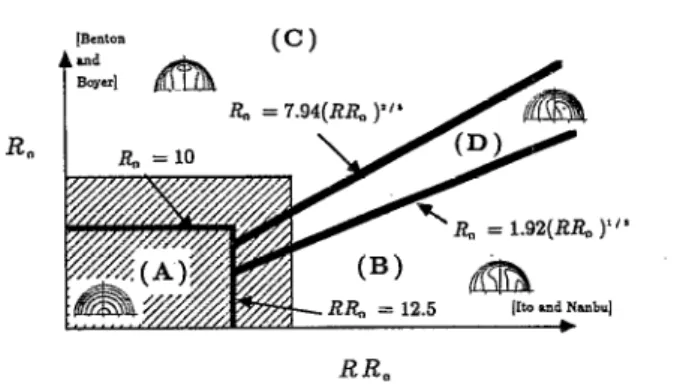
flow regimes as- follows. (1) Regime A: the flow is essen- tially axisymmetric and is similar to that of the Poiseuille solution when both N,N, and N: are small. (2) Regime B: In the regime where N% is small but NRNn is not, the effect of rotation is to skew the parabolic axial velocity profile (Hagen-Poiseuille) toward the outside, i.e., rotation moves the location of maximum axial velocity outward along 8=0” in Fig. 1. (3) Regime C: In the regime where N,N, is small but Nt is not, the effect of rotation is to reduce the centerline velocity and produce an axial velocity prolile with two maxima, one along B=90” and one along 0=270”. (4) Re- gime D: If both N,N, and Ni are of significant size, the axial velocity profile is skewed with two maxima, which occur symmetrically in the first (O”~K90”) and the fourth (270”<8<360”) quadrants in Fig. 1. These four flow re- gimes were confirmed and extended by Lei and Hsu7s3 cal- culation for the perpendicular rotating case (cr=90”). Through a series of scaling analyses and a detailed calcula- tion, Lei and Hsu were able to classified quantitatively the parameter regimes for the above four flow regimes. The bound&y Iayer analysis by Benton and Boye? belongs to regime C and that by Ito and Nanbu6 belongs to regime B. Regime D is the intermediate region between regime B and C. The relative positions in the parameter space for these four flow regimes are sketched in Fig. 2 in terms of the present parameters

(Rn

and

RnR)

according to Lei and Hsu.~ The regions studied analytically by Berman and MO&OS, Benton and Boyer,’ and Ito and Nanbu6 are shown in Fig. 2. The region studied numerically by Lei and J$u* bridges the above three “analytical” regions, and cover the whole region studied by Berman and MO&OS. Also shown in Fig. 2 are the typical norma!ized axial velocity contours in the

r’8

plane for these four flow regimes. Recall that the flow is symmetric about the plane y ’ =0 in Fig. 1, and here only half of the

rtJ

plane is shown in Fig. 2. The contour values start- ing from the semicircular boundary are w ‘Iw;, = 0,0.2,0.4, 0.6, 0.8, and 0.95, respectively, where ~6~ is the maximum axial velocity. The location of wk,, is denoted by a circular dark point in each case. Typical three-dimensional sketches

-0;

_Y’

₇

v-

0

r*

X’ ;,

(top view) (side view)

FIG. 1. The coordinates of the rotating pipe flow in the present study.

of the axial velocity profiles for the above four flow regimes can be found from Berman and Mockro~.~

The previous experimental studies for this problem are rare in comparison with the analytical and numerical works. Benton and Boyers obtained the axial velocities along the x’ axis on the symmetric plane for ten cases ranging from

Rn=1250-2778

with

R, = wAa/u M 290 - 335

(i.e.,the

regime C) by measuring the axial motion of the dye from photographs taken on a rotating table, where WA is the axial velocity on the pipe axis. They found that their measure- ments were in agreement with their analyses within 10% discrepancies for

-0.46dla<0.46.

Ito and Nanbu6 mea- sured the reduced pressure drop at the fully developed region for wide ranges of

R

and

Rn.

They also measured a profile for the axial velocity distribution along the x’ axis when

R

=2000 and

Rn=250

(regime B) using a pitot tube mounted with the pipe system on a rotating mechanism.

Although the basic physics of the laminar fully devel- oped pipe flow in a rotating frame is clearly understood through the previous studies mentioned above, a rigorous experimental validation for the four flow regimes is still lacking in the literature. The primary goal of this paper is thus to provide such validation by measuring the axial veloc- ity for different parameters. This paper also aims to study the asymptotic nature of the slow flow in a rapidly rotating pipe

1 t/r

b-4

RR.

FIG. 2. The relative positions of the four flow regimes (A, B, C, and D) in the parameter diagram for the present rotating pipe flow together with the typical sketches of the axial velocity contours for different regimes. The shaped region was studied by Berman and MO&OS. Also indicated in the diagram are the regions for the validity of the asymptotic resuIts for the rapid flow in a slowly rotating pipe by Ito and Nanbu and the slow flow in a rapidly rotating pipe by Benton and Boyer.

(Benton and Boyers) and the rapid flow in a slowly rotating pipe (Ito and Nanbu’). Besides, the calculations by Duck7 are different from those by Lei and Hsus for

R,=5

and

R =430

- 1107. The present study also provides an experimental in- vestigation to those cases to see if there may exist dual so- lutions for such parameters. The results of the present study have engineering applications in the design of the cooling channels inside the rotating blades of gas turbines (see Morris”), and of some piIje flow systems in a rotating frame such as those on a spinning satellite.

II. EXPERIMENTAL DETAILS T

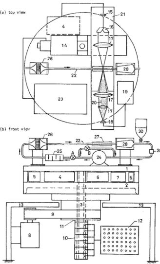
As the flow occurs in a rotating frame, both the circulat- ing pipe flow system’ and the devices for velocity measure- ments were mounted on a rotating table for the experiment. The rotating table, the measuring device’and the circulating pipe Aow system are sketched in Fig. 3, and are described as follows.

The rotating table was made of two circular disks with 80 cm in diameter and 2.3 cm in thickness. The upper disk was made of steel and the lower disk was made of cast iron, and both disks were mounted on’ a vertical hollow shaft with outside diameter 5 cm. The spacing between the two disks is 11 cm. The space-between the two disks was employed to install the laser driver of the measuring device, the balancing masses for steady and stable rotation, the signal connection board and the electric power module. The rotating table was driven by a dc motor through a belt. The rotation speed could be varied from 0.005 - 1 rps (revolutions per second) by al- tering the input voltage of the dc motor, and was measured by recording the time spent in a given number of revolutions using a stop watch. The upper disk was drilled with holes such that the measuring device and the circulating pipe flow system could be mounted on it for the experiment. In order to transfer the measuring signals from the rotating frame to the outside inertial frame, a slip ring with 48 poles was in- stalled at the bottom part of the shaft. The wires connecting the poles of the moving (inner) part of the slip ring and the signal connection board on the rotating table were placed and fixed inside the hollow shaft. The instruction signals could also be sent into the rotating frame from outside through the slip ring. There are up to 48 signals that can be transferred between the rotating and the inertial frame. The stationary (outer) part of the slip ring was connected to a signal con- nection board in the inertial frame, which was installed on the case of the rotating table. The case is a square box made of steel plates, which contains the bottom part of the shaft, slip rings, motor, belt, and wires. A slip ring for power sup- ply was also installed on the shaft and connected to the elec- tric power module between the two disks. Several transform- ers are included in the power module such that the power module can provide dc 5 V, dc 12 V, ac 100 V, and ac 110 V power sources to the devices installed on the rotating table. The devices for velocity measurements include a for- ward scattering diode laser Doppler anemometer (LDA) sys- tem and a three-axis traversing table. The.diode laser LDA system is a light weight, compact device in comparison with the traditional He-Ne and argon-ion laser LDA system. There are two parts of the present LDA system, the part

(a)

(b)

I 1

top view _{-...Jdy--t--&q=21}

FIG. 3. Sketch of the apparatus of the present study. The components are (1) upper disk, (2) lower disk, (3) shaft, (4) laser driver, (5) balancing masses, (6) signal connection board on the rotating frame, (7) electric power module, t8) dc motor, (9) belt, (10) slip ring for transfering the signals, (11) slip ring for transferring the electric power, (12) signal connection board on the in- ertia frame, (13) case, (14) three-axis traversing table, (1s) laser head, (16) beam splitter, (17) focus lenses, (18) avalanche photodiode (APD), (19) power supply for the APD receiver, (20) scattering light, (21) aluminum plate, (22) test section, (23) control box of the traversing table; (24) pump, (25) flow buffer, (26) honeycomb and flow contractor, (27) square box, (28) diffuser, (2.9) flow meter, and (30) reservoir.

installed on the rotating table [see Fig. 3(a)] and the signal processing part in the inertial frame. Consider first the part installed on the rotating table, which includes a laser driver, laser head, collimator, prism pair, beam splitter, three. focus lenses, several ring mounts, and a APD (avalanche photodi- ode) receiver. The diode laser generates a 40 MW laser beam with wavelength 834 nm. The laser beam which is emitted from the laser head is separated into two parallel beams by the beam splitter. These two parallel beams are then focused through a focus lens to form a measuring volume. The Dop- pler signals are collected through two focus lenses, and are received by the APD receiver. The APD receiver includes a power supply and an avalanche photodiode with 150 Hz to 125 MHz bandwidth, 500-1000 nm spectral range and a 200 pm pinhole. The laser head, the lenses, and the avalanche photodiode were all fixed on an aluminum plate once they had been adjusted, and were mounted along the x’ axis of the

TABLE I. The equation for the path traced out by the center of the measur- ing volume withinx’+y’<l for (a) m,=1.52 (quartz glass) and m,=1.452 (85% glycerin-15% water solution), ‘and (b) m,=1.52 (quartz glass) and tnW= 1.33 (water).

(a) me=152 and m,=1.452

h path with square box path without square box 0.1 y=o.ooo 349x+0.100 0.2 y=O.OOO 726x+0.200 0.3 y=O.OOl 17x+0.300 0.4 y=O.OOl 73x+0.400 0.5 y=o.o02 50x+0.500 0.6 y=O.O03 67x+0.600 0.7 y=O.O05 66xf0.70d 0.8 y=O.O09 72x+0.800 0.9 y=O.O212x+O.892 (b) m,=1.52 and m,=1.33 y=-0.0286x+0.0689 y=-0.0578x+0.138 y=-0.0882n+0.208 y=-0.121x+0.278 y=-0.156x+0.349 y=-0.196x+0.421 y=-0.244x+0.496 y=-0.303x+0.575 y=-0.385x+0.664 0.1 y=o.ooo 973x+0.100 y=o.ooi d2x+0.200 y=-0.0223x+0.0752 0.2 y=-0.0450x+0.151 0.3 y=O.O03 23x+0.300 y= -0.0686x+0.226 0.4 y=o.o04 74x+0.400 y= -0.0939x+0.303 0.5 y=O.O06 77x+0.500 y=-0.122x+0.378 0.6 y=O.O09 73x+0.600 y= -0.153x+0.456 0.7 y=0.0145x+0.700 y=-0.190x+0.536 0.8 y=O.O237x+O.801 y=-0.237x+0.618 0.9 y=O.O464x+O.901 y= -0.301x+0.706

W

2.5

I I I

2

1.5

1

0.5

1 I

0.5

1

X

FIG. 4. The variations of the dimensionless axial velocity (w = w’lw;) with x( =~‘/a) in an inertial frame. The Poiseuille solutionis represented by the curve. The present measurements are represented by the data points, 0 for R=94.3, + for R=125, and X for R=457.

2.5

2

1.5

W

1

0.5

-I

n

/ ,...,... ;. .,....,,.,... j ; I 1 \ ,, I l-

--1

-0.5

0

0.5

1

X

FIG. 5. Comparison of the dimensionless axial velocity distributions be- tween the numerical solution by Lei and Hsu and the present measurements for different test sections and different downstream locations at R = 12.5 and Rn= 1 (regime A). The numerical solution is represented by the curve. The measurements are represented by the data points, the circles (0) for 2a = 1 cm and r’/a =90, the plus symbols (+) for 2a =3 cm, and ~‘/a =28, and the cross symbols (X) for Lx=3 cm and z’/a=21.8.

three-axis traversing table. The directions of the axes of the traversing table are the same as those in Fig. 1, with the x’ axis perpendicular to the axis of the test section discussed later in the circulating pipe flow system. As the laser light of the diode laser is invisible, an IR viewer was employed to adjust the laser beams and the measuring volume. The tra- versing table together with its control box were mounted on the upper disk of the rotating table. The motion of the tra- versing table (and hence, the measuring volumej was con- trolled by an 80286 personal computer in the inertial frame through the slip ring, and thus the measuring volume of the LDA system could be moved as desired while the rotating table was in motion. The power supply of the APD receiver was also mounted on the upper disk of the rotating table. The Doppler signals received by the avalanche photodiode were amplified by an amplified circuit built in the box of the power supply of the APD receiver, and then tranferred to the signal processing part of the LDA system in the inertial frame through the slip ring. The signal processing part in- cludes a high-pass/low-pass filter, a digital burst correlator, an 80486 personal computer, and an oscilloscope. The Dop- pler signals went through the filter, the correlator and then the personal computer for data processing. The Doppler sig-

I I ,

a-

X

1

FIG. 6. Comparison of the dimensionless axial velocity distributions be- tween the numerical solution by Lei and Hsu and the present measurement at R =704 and Rn=lO (regime B). The numerical solution is represented by the curve, and the experimental results are represented by the circles.

nals were monitored by using the oscilloscope during the experiment.

The circulating pipe flow system which was mounted on the upper disk of the rotating table is sketched in Fig. 3(b). It includes two loops: the primary loop for the main circulation and the secondary loop for the tlow regulation. The fluid in the pipe flow system was pressurized by a pump. The fluid which left the pump first meets a T junction between the primary and the secondary loop. The flow rate of the primary loop and that of the secondary loop could be controlled by the valves A and B. When a large f-low rate was required in the test section, valve B was closed such that the secondary loop was disabled. On the other hand, most of the fluid that left the pump would go through the secondary loop if a small steady low tlow rate was required in the test section. Besides valves A and B, the flow rate could also be regulated by varying the input voltage of the ac motor which drove the pump. The fluid through the valve A would enter a flow buffer, which is a large hollow cylinder with alternating blocking plates in the flow direction. The primary role of the buffer was to trap the gas bubbles in the circulating pipe flow system, and the bubbles were removed through a ventilating valve located on the top of the buffer. In order to generate a

“uniform” flow at the inlet of the test section, the fluid from the buffer was let to flow through a honeycomb and a smooth contractor before entering the test section. The test section is

1.6

0,6

X

. . . )

1

1.8

1.6

1.4

1.2

1

W

0.8

0.6

0.4

0.2

0

0

.: I , I

0.2

0.4

0.6

Y

- --

0.8

1

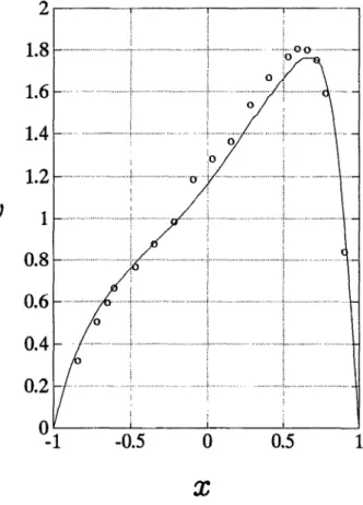
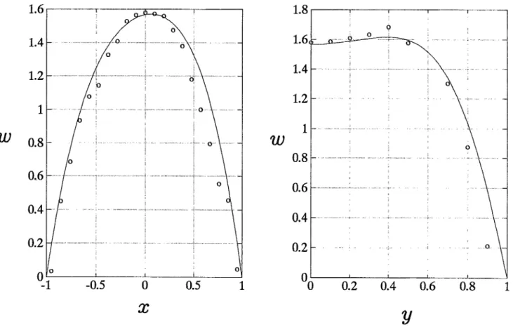
FIG. 7. Comparison between the numerical solutions by Lei and Hsu and the present measurements at R =3.03 and 17.4 (regime C). The numerical solutions are represented by the curves, and the measurements are represented by the circles.

a circular tube made with quartz glass, and the LDA mea- surements were taken at a downstream location sufficiently far from the inlet. For the laminar circular pipe flow in an inertial frame, the entrance length

L,,

defined as the axial distance from the inlet required for the axial velocity on the pipe axis to reach 99% of the Poiseuille value, is

L,

-w

2a

,+“,:“,,R +O.l12R,

(1)

according to Shah and London.” In case the pipe flow oc- curs in a rotating frame,

L,

can be reduced substantially by the rotating effect, according to the calculation of the parabo- lized Navier-Stokes equations (Chen”) and the full Navier- Stokes equations (Yang’*). The determination of whether the flow reaches the fully developed state for a given set of pa- rameters was estimated by using the results of Shah and London,” Chen,” and Yang,” and by comparing the mea-

surements at two neighboring axial locations. The two laser beams forming the measuring volume entered the test section along a plane with y ‘==const in Fig. 1. The path of the laser beam was deflected by the curvature of the tube except on the y ’ =0 plane, i.e., the horizontal movement of the travers- ing table along the x’ axis (with y ’ and z’ fixed) makes the center of the measuring volume inside the tube traces out a straight path with finite slope in the x’y ’ plane except y ’ =O. In order to reduce the slope of the path of the measuring volume, a square box was built outside the circular tube, and the space between the tube and the wall of the box was filled

with the same kind of fluid as that inside the test section. The two side walls perpendicular to the incoming laser beams were made of optical glass, and the other four sides of the square box were made of Plexiglas. Two holes were drilled on the upper wall of the square box for fluid filling and gas removement. The fluids employed in the present experiment were water and glycerin-water solution. The glycerin-water solution was seeded to enhance the laser scattering during the experiment. No seeding was required when the working fluid is water. Although the refractive indexes of the water (m,) and the glycerin-water solution (ms) are still slightly different from that of the quartz glass (mg), the slope of the path traced out by the measuring volume is small after using the square box. Assume that the traversing table moves along the x’ axis in a plane y ‘=h’=const. Let

x=x’la, y=y’la

and

h

=

h

‘/a. On using the principle of Fermat for refraction, the paths traced out by the center of the measuring volume inside the test section with or without the square box were evaluated and listed in Table I for

ms=1.452 (85%

glycerlin-15% water), m,=1.33,

m,=1.52,

a=1.5 cm, and t=0.125 cm, where t is the thickness of the tube (the test section). It was found that the slope of the path is still very small even when

h=0.9

for the case with square box. There were three types of test section employed for different pa- rameters in the present experiments: (1)

2a

= 1 cm and

L = 60

cm, (2) 2a=2 cm and L =120 cm, and (3) 2a=3 cm and L =50 cm, where L is the axial length of the test section. The fluid that left the test section went through a diffuser, an

+ooo

; h=O ..I.. . . ..(J .i

1.5 ...

kc o...! O

..

w

1 -I*“;

...

... i..

...

.! .. ...

\$i

.

1

W

W

2r

X

_X

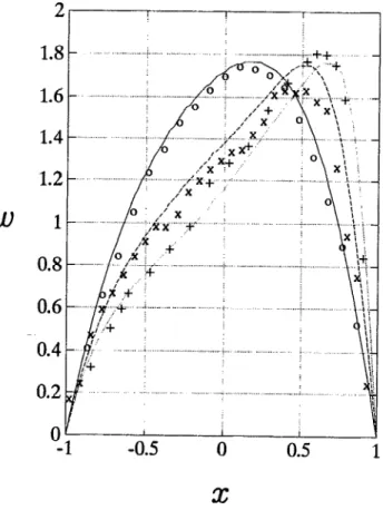
FIG. 8. Comparison of the dimensionless axial velocity distributions between the numerical solutions by L.ei and Hsu and the present measurements at R =4.73 and Rn=20 (regime D) at different values of h. The numerical solutions are represented by the curves, and the measurements are represented by the circles.

integrated-type flow meter and then entered the pump to complete a circulation loop. The output signal of the flow meter was sent outside from the rotating frame through the slip ring to a timer. A small reservoir with cover opening to the surrounding was also connected to the circulating system for filling the fluid and removing the gas. A thermometer could be inserted into the pipe flow system from the reser- voir to measure the temperature of the flow.

There was no temperature control system in the present experiment. The whole system was let to run for a suffi-

Phys. Fluids, Vol. 6, No. 6, June 1994 Lei et a/.

ciently long time (more than 30 min) such that the system was in thermal equilibrium before taking the data. The heat generated by the pump (a steady heat source of the circulat- ing flow system) was removed by a fan installed on the ro- tating table, so that the temperature of the flow was limited to within 33 “C. The viscosities of the testing fluids at differ- ent temperatures were measured separately by using a digital viscometer together with a constant temperature bath. The viscosity of the fluid was determined once the temperature of the circulating system was measured. Thus for a given test

X

FIG. 9. The variations of the dimensionless axial velocity distributions for different values of R at Rn= 10. The numerical result by Jki and Hsu and the present experimental result are denoted by solid line and circles (0) for R = 10.9, by dash line and cross symbols (X) for R =94.3, and by dotted line and plus symbols (+) for R =704, respectively.

section (given a), the two independent dimensionless param- eters,

R

and

Rn,

for a given experiment were known after the volume flow rate (Q) and the rotation speed (sl) were measured. The flow meter was calibrated before doing the experiment. Two methods of calibration were employed in the present study. For water, the flow meter was calibrated by measuring the volume of the fluid flow through the meter for a period of 100 s. The variations of the reading of the flow meter with the actual flow rate (Q) was linear up to Q-100 cm3/s. As the viscosity of the glycerin-water solution varies significantly with temperature and moisture in the surround- ing, the flow meter for cases with such fluid was calibrated by using the present circulating pipe flow system and the LDA system without turning the rotating table. For a given reading of the flow meter, the axial velocity at the pipe axis (WA) in the laminar fully developed region was measured, which equals to 2wk, according to the Poiseuille solution. The flow rate Q then equals to ,*wL. The latter calibration method using the pipe flow velocity measurement was also employed for water in order to ensure that both calibration methods give the same result. The data for the flow meter calibration can be found from Lin.13 The effect of rotation on the reading of the flow meter was studied by varying the position of the flow meter on the rotating table (the flow meter is connected to the diffuser and the pump by soft tubes). It was found that the readings were essentially the

same for different locations of the meter within the range of rotation speed for the present study. The alignment of the optics, the installation of the circulating pipe flow system and that of the LDA system were checked by comparing the measurements of the axial velocity profiles at different Rey- nolds number and f-1=0 with the exact Poiseuille solution. The results for three different measurements along the x’ axis with different Reynolds numbers are plotted in Fig. 4 together with the Poiseuille solution. The experiment with

R=457

was carried out with water, and the remaining two

measurements were carried out with glycerin-water solution. The experimental data are in good agreement with the exact solution.

III. RESULTS AND DISCUSSION

The four fow regimes mentioned above were validated by the following four cases: (1)

R

= 12.5,

R,=

1 (regime A, Fig.

5); (2) R

=704, Rn=10 (regime B, Fig. 6); (3)

R =3.03,

R,=17.4 (regime C, Fig. 7); and (4)

R=4.73, R,=20

(re- gime D, Fig. 8). The numerical solutions according to Lei and Hsu8 for these four cases are also shown in Figs. 5-8. The test fluid for the experiment is water for case (B) and 85% glycerin-U% water solution for cases (l), (3), and (4). Let w = d/w;, and recall that x=x’/u and y =y’la. Fig- ure 5 shows three measurements for w along the x axis for case (1) at different downstream axial locations and with different test sections. It is found that the experimental re- sults are essentially parabolic, and agree nicely with one an- other and with the numerical solution. The flow in regime B is characterized by a skewed axial velocity profile similar to that in curved pipe, with the maximum value occurs on the positive x axis. Figure 6 depicts the dimensionless axial ve- locity distribution ( W) along the x axis for case (2), and there are good agreement between the experimental results and the numerical calculations. Figure 7 illustrates the dimensionless axial veIocity distributions along the x axis and that along they axis. Same as the numerical solutions, the experimental measurements indeed indicate that the axial velocity is es- sentially symmetric about the y axis and possesses a maxi- mum at a positive y location. Note that the flow is symmetric about the symmetric plane y =O, and here only the result for yr0 is shown in Fig. 7(b). The symmetry of the flow field about y =0 had been checked experimentally, and the results can be found form Lin.13 Figure 8 shows the axial velocity distributions along the x axis for different values of h (see Table I). Here h is the dimensionless distance of the laser beam from the symmetric plane y =0 outside the test section, which can be controlled and adjusted easily by the move- ment of the three-axis transversing table. The measurements in Fig. 8 are the axial velocities along straight lines with finite slopes in the xy plane, and thus two position variables are required for illustrating the measurements. Here we em- ployed x and

h.

The equations of the straight lines where the measurements were taken are listed in Table I for different values of

h.

The measurements are in agreement with the calculations, and the axial velocity is skewed toward the pressure (positive x) side with the maxima occur slightly on the right of the y axis.

0.8

t

W’

-

0.6

20:

0.4

Si

_-0.5

₀

0.5

1

X

1.2

1

0.8

20’

-

0.6

wi

0.4

0.2

OL

! 1 xmqx, +-J&G j QP# 0 k ‘+.-.. ,.,.... i 0 0 i i. ,. ,... .+. .j ,... fi ! ..,.. . ..t ,.. .i .,... i I I f

0

0.2

0.4

0.6

0.8

1

Y

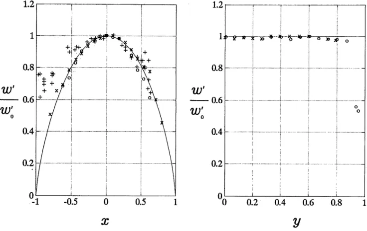
FIG. 10. Study of the asymptotic case for R$-1 and R,%R. The asymptotic solutioris by Benton and Boyer are represented by solid lines. The measurements by Benton and Boyer are represented by the plus symbols (+). The present measurements at R,=1250 are represented by the circles (0) and the cross symbols (X) for R=250 and R =452, respectively.

As discussed in Lei and Hsu,* the different flows in the four different flow regimes are resulted from the various ef- fects of the secondary flow on the main stream via the con- vection and the Coriolis mechanisms, and can be understood clearly through a scaling analysis of the equations governing the fluid motion. There are four terms in the axial momentum equation for the present fully developed pipe flow in the rotating frame in Fig. 1 (see Lei and Hsu’): the convection term due to the secondary flow, the pressure term which drives the flow, the Coriolis term and the viscous term. The flow is axisymmetric and possesses a maximum on the pipe axis when both the convection and the Coriolis effects are absent. The convection effect tends to move the location of the maximum axial velocity along the positive x axis, while the Coriolis effect tends to reduced the axial velocity near the center and produces a dumbeli-like profile with two maxima located symmetrically on the positive and negative y axis, respectively. For regime A, both the convection .and the Co- riolis terms are negligible, the flow is thus essentially axi- symmetric and similar to that of the Poiseuille solution. For regime B, the convection term is of the same order as the pressure and viscous terms, and pushes the location of the maximum axial velocity toward the pressure side (positive x). For regime C, the Coriolis term, the pressure term and the viscous terms are of equal importance, and thus the axial velocity shows a dumbell-like profile. All of the four terms are significant for the tlow in regime b. Both the convection

and the Coriolis mechanisms are acting on the flow, and thus the flow is skewed toward the pressure side with two maxima in regime D. The parameters for the results in Figs. 5-8 are selected such that they are located separately in the four different regimes in Fig. 2. As the magnitudes of the terms in the axial momentum equation depend continuously on the parameters

R

and

R,,

the flow in one regime transits smoothly to the other regime as the parameters vary. Figure 9 shows that the maximum value of the axial velocity profile shifts continuously toward the pressure side as

R

increases (the convection effect increases) for Ro=lO, and the mea- surements agree nicely with the calculations. Other results of the variations of the flow as the parameters vary may be found from Figs. 10-12. Since the calculations by Lei and Hsu8 were validated experimentallv by the results in Figs. 5-9 and some other results in Lin-,13 detailed variations of the flow (including both the axial velocity and the secondary stream function) with the parameters can be found from Lei and Hsu. A scaling analysis for illustrating the essential physics of the flow phenomena can also be found from Lei and Hsu.

After the validation of the existence of the four flow regimes, we study the asymptotic case for slow flow in a rapidly rotating pipe when l?oSi and

R,SR,

i.e., the lim- iting case for regime C. Benton and Bayer’ proposed that the flow field can be analyzed by separating it into two regions: the core region and the boundary layer. The inertia force is

2

1.8

1.6

1.4

1.2

w

1

0.8

0.6

0.4

0.2

X

1

2

1.8

1.6

1.4

1.2

w

1

0.8

0.6

0.4

0.2

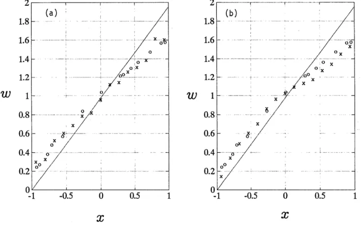
FIG. 11. Study of the asymptotic case for RnQR and RR,+l. The asymptotic solution by Ito and Nanbu is represented by the solid straight line. The experimental results for R =2000 and Rn=Z50 by Ito and Nanbu are represented by the circles (0). The cross symbols (X) in (a) are the present measurements for R =2000 and Rn=250 (K,-4X lo6 and A=O.125), and that in (b) are the present measurements for R =2500 and Rn=Z50 (K,=5X10b and A=O.l).

not significant in either region. The thickness of the bound- ary layer is of order

aIRa .

“’ The core region is geostrophic with the axial velocity distribution satisfying

w’/w;)= (1 -x2)3’4, ₍₂₎

according to Benton and Boyer, where WA is the axial veloc- ity along the pipe axis and is the maximum value in the asymptotic analysis. Note that w ’ is independent of y, ac- cording to Eq. (2). The calculations by Lei and Hsu’ show that Eq. (2) is valid for

RnIR

aO(10) and ]yj ~0.5 when

Rn=lOO.

However, the maximum values of w’ occur at

r’/a=0.75 and 6=+90” instead of at

r’=O

due to the vari- ous effects of the Coriolis force on the boundary layer flow at different azimuthal locations, which was explained by Lei and Hsu through a scaling analysis and is in qualitative agreement with the perturbation analysis by Berman and Mockro~.~ Benton and Boye? verified their analytical result in Eq. (2) by carrying out a series of measurements of the axial velocity distributions on the symmetric plane ranging from

Rn=12S0-2778

and

R,=290-335

as mentioned in Sec. I. Note that

R,

is greater than

R.

Due to the limitation of their measuring technique at that time, Benton and Boyer found that their measurements agree with their analysis within 10% error for -0.46eGO.46. Figure 10 shows the present measurements of the axial velocity distributions along the x and the y axis together with the asymptotic so- lution [Eq. (2)] and the experimental results by Benton and

1980 Phys. Fluids, Vol. 6, No. 6, June 1994 Lei et

al.

Boyer. The parameters for the present measurements are

RQ=1250

and

R=2.50

and 452. The present measurements

are in good agreement with the asymptotic solution. It is found that the asymptotic solution for

R+-I

and

Rn%=R

by Benton and Boyer is valid for ]y]G0.85’when

R,/R>3

and Ro = O( 1 03), which is a larger region for y in comparison with that for

Rn=

0( IO’) (see Lei and Hsu’) as expected. Also the lower limit of the validity of the asymptotic ‘result

for

RnIR

is reduced as

R,

increases by comparing the

present experimental results with the calculations by Lei and Hsu.

For the rapid flow in a slowly rotating pipe when

Kl=8RRn&l

and

A=RnIR4

(i.e., the limiting case for

regime B), Ito and Nanbu6 proposed that the how can be solved by separating it into two regions: (1) a thin boundary layer with thickness of order

aKi’4

near the wall of the pipe and (2) a frictionless core where the flow is influenced by inertia and pressure forces. They found that the axial velocity is linear with x in the core, and provided a set of experimen- tal data for

R=2000

and

Rn=‘2S0

(i.e., K,=4X106 and A=O.125) to support their theory. The measurements agree fairly with the theory, as shown in Fig. 11(a). Also shown in Fig. 11(a) is the present experimental results with the same parameters as those in Ito and Nanbu. The present experi- mental result agrees nicely with the measurement by Ito and Nanbu. As the present measurement technique is different from that in Ito and Nanbu, the discrepancy between the

1.8 - 1.6 - 1.4 - 1.2 - l- * CM--~ x,

W

X

asymptotic theory and the experiments is not primary due to the accuracy of the measurements. In order to see if there may exist better agreement between the asymptotic theory and the experiments as either

K,

increases or A decreases, we have carried out four additional measurements with

Kl

rang- ing from 3X106 to 5X106, and A ranging from 0.1 to 0.167. Note that for laminar flow, there exist an upper bound for

Kl

for a given value of A, since the flow may become unstable if

K,

exceeds a critical value (see Ito and Nanbu6). The dis-

X

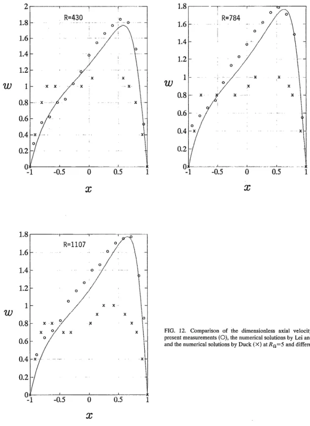
FIG. 12. Comparison of the dimensionless axial velocity between the present measurements (0), the numerical solutions by Lei and Hsu (curves), and the numerical solutions by Duck (X) at Rn=5 and different values of R.

crepancies among the four additional measurements and the experimental results in Fig. 11(a) are within experimental uncertainties. A typical result for Kr=5X106 and A=O.l iR =2500 and

Rn=250)

is plotted in Fig. 11(b) together with the asymptotic and the experimental results by Ito and Nanbu. It is found that the two experimental measurements in Fig. 11(b) with different parameters give almost the same result. Therefore, the “slightly” disagreement between the asymptotic solution and the experimental measurement is

probably due to the inherent nature of the assumptions in the asymptotic analysis. As convection is important in the core, the discrepancies between the asymptotic and the experimen- tal results in Fig. 11 are assumed to be mainly due to the detrainment of the fluid from the boundary layer at x=-l and the entrainment of the fluid into the boundary layer at x=1.

Although the dimensionless volume flow rate calculated by Duck’ agrees fairly with that by Lei and Hsu’ for the same values of

Rn

and

R,

the detailed flow field between these two calculations are significantly different from each other for

Rn=5

and

R=430,

784, and 1107, as discussed in Lei and Hsu. The flow for such cases belong to regime B, which is similar to the tlow in a loosely coiled pipe. As there may exist dual solutions in the curved pipe flow for large Dean number (see Dennis and Ng14), it is not certain that whether the difference between the calculations by Duck and that by Lei and Hsu is the consequence of the existence of dual solutions. Figure 12 shows the measurements of the axial velocity distributions along the ,x axis for the above three cases together with the numerical results by Duck7 and by Lei and Hsu.’ The results by Duck were obtained from their axial velocity contours. It is found that the experimental results agree with the solutions by Lei and Hsu. In order to check if the “disturbances” of the system can affect the ex- perimental results in Fig. 12, we first adjusted the rotating table to the speed corresponding to

R,=5,

and then adjusted

R

to the given value in two ways. One was to increase the pumping power (i.e., the volume flow rate) from zero, and the other was to decrease the volume flow rate from an initial large value. Both measurements gave essentially the same results.

Most of the experimental results shown in this paper were repeated twice. There are several resources of experi- mental uncertainties for the present measurements. The un- certainty associated with the diode laser, the optics and the electronics was estimated to be about 2% for the velocity measurement sufficiently far from the wall. Such uncertainty is larger for the measurement near the wall due to the veloc- ity bias, and has been corrected during data reduction. The uncertainty for the near-wall measurement was then esti- mated to be about 6%. The uncertainty for the rotation speed was about 1%. The uncertainty for the volume flow rate was about 2%. The uncertainty for the viscosity (mainly due to the temperature variation) was about 3%. The uncertainty associated with the orthogonality between the laser beam and the side wall of the square box for the test section was esti- mated to be 4% for region not near the wall. Such uncer- tainty could be large for large y for the flow in regime C (as indicated by Figs. 7 and lo), since the location of the mea- suring volume which is expected to be located in the core, according to Table I, may fall actually inside the boundary layer.

In this study, an experimental system was set up for studying the pipe flows in a rotating frame, which includes a rotating table, a circulating pipe flow system, and a diode laser LDA system together with a three-axis traversing table. The existence of the four flow regimes has been validated experimentally by measuring the axial velocity distributions for different parameters. Detailed variations of the flow with parameters and the essentially physics of the flow phenom- ena according to the previous analyses and calculations can then be accepted and employed with confidence. The asymp- totic nature were also studied experimentally for the slow flow in a rapidly rotating pipe (R$=-1 and

R,SR)

by Ben- ton and Boyer and for the rapid flow in a slowly rotating pipe

(RR,%1

and

R% Rn)

by Ito and Nanbu. It is found that the

asymptotic result by Benton and Boyer is valid when

RnJR

>3 for

Rn

= O( 1 03). However2 the agreement between

the asymptotic result by Eto and Nanbu with the experiment is fair due to the inherent nature of the assumption made in the analysis. A preliminary investigation on the dual solution problem for small

Rhl

and large

R

had also been carried out, and it was found that the solution is unique up to

R =

1107

for

Rn=5.

The experimental system in the present study can

be modified to study the entry flow and the turbulent flow in a rotating straight pipe. The work for the entry flow is in progress.

‘S. N. Baura, “Secondary flow in a rotating straight pipe,” Proc. R. Sot. London Ser. A 227, 133 (1954).

sG. S. Benton, “The effect of the Earth’s rotation on laminar flow in pipes,” Trans. ASME: J. Appl. Mech. 23, 123 (1956).

3J. Berman and L. E MO&OS, “Flow in a rotating non-aligned straight pipe,” J. Fluid Mech. 144, 297 (1984).

4K Mansour, “Laminar flow through a slowly rotating straight pipe,” J. Fluid Mech. 150, 1 (1985).

‘G. S. Benton and D. Boyer, “Flow through a rapidly rotating conduit,” J. Fluid Mech. 26, 69 (1966).

‘H. Ito and K. Nanbu, “Flow in rotating straight pipes of circular cross section,” Trans. ASME: J. Basic Eng. 93, 383 11971).

7P. W. Duck, “Flow through rotating straight pipes of a circular cross sec- tion,” Phys. Fluids 26, 614 (1983).

“U. Lei and C, H. Hsu, “Flow through rotating straight pipes,” Phys. Fluids A 2, 63 (1990).

“W. D. Morris, Heat Transfer and Fluid Flow in Rotating Coolant Chan- nels (Wiley, New York, 1981), Chap. 6.

“‘R K Shah and A. L. London, Laminar Flow Forced Convection in Ducts

(Acabemic, New York, 1978).

“R. H. Chen, “Calculations of the entry flow through a rotating straight pipe,” Master thesis, National Taiwan University, 1989.

“C. Y. Yang, “Calculations of the fluid flow and heat transfer in a rotating straight pipe,” Master thesis, National Taiwan University, 1990. t3M. R. Lin, “Experiments on the flow through a rotating straight pipe,”

Master thesis, Natlonal Taiwan University, 1992.

t4S. C. R. Dennis and M. Ng, “Dual solutions for steady laminar flow through a curved tube,” Q. J. Mech. Appl. Math. 35, 305 (1982).