國 立 交 通 大 學
電 信 工 程 研 究 所
碩 士 論 文
運用在無線物聯網的位置更新之
樹狀資料結構最佳修剪演算法
Optimal Tree Pruning for Location Update in
Machine-to-Machine Communications
研究生:鄭青佩
指導教授:高榮鴻 博士
運用在無線物聯網的位置更新之
樹狀資料結構最佳修剪演算法
Optimal Tree Pruning for Location Update in
Machine-to-Machine Communications
研究生:鄭青佩
Student: Ching-Pei Cheng
指導教授:高榮鴻
Advisor: Rung-Hung Gau
國立交通大學
電信工程研究所
碩士論文
A Thesis
Submitted to Institute of Communications Engineering
College of Electrical and Computer Engineering
National Chiao Tung University
in Partial Fulfillment of the Requirements
for the Degree of Master of Science
in
Communications Engineering
June 2013
運用在無線物聯網的位置更新之
樹狀資料結構最佳修剪演算法
研究生
:鄭青佩
指導教授
:高榮鴻
國立交通大學電信工程研究所碩士班
摘
要
在本篇論文當中,我們提出了運用在無線物聯網之下,使用剖析
樹資料結構的位置更新演算法。在無線物聯網的通訊網路環境中,可
能會有非常大量的通訊設備
(MTC設備
)聚集在同一個區域當中,假
使每個
MTC設備都採取定期更新位置的方式回報給伺服器,如此一
來就會造成伺服器端雍塞的情況。根據消息理論,跟傳統的定期回報
位置更新訊息方式比較起來,比較有效率的方法是
:唯有在需要增加
新節點到剖析樹中的時候,
MTC設備才需要回報位置更新的資訊。
進一步而言,由於
MTC設備的記憶體容量通常不大,而且使用電池
供電,需要避免能源的消耗,因此我們提出了一個樹狀資料結構最佳
修剪演算法,此演算法可以最小化記憶成本和能源成本的權重和。此
外,我們推導出此演算法的計算複雜度很小,是可以運用在實際的系
統上的。最後,我們同時使用了分析結果和模擬結果來證明我們所提
出的方法。
Optimal Tree Pruning for Location Update in
Machine-to-Machine Communications
Student : Ching-Pei Cheng Advisor : Rung-Hung Gau
Institute of Communications Engineering
National Chiao Tung University
Abstract
In this thesis, we propose a parsing-tree-based location update scheme for wireless Machine-to-Machine (M2M) communication. In M2M communica-tion networks, there might be a large amount of Machine-Type-Communicacommunica-tion (MTC) devices in a small area. If each MTC device periodically performs location update, the MTC server might be overloaded. According to Informa-tion Theory, in comparison with periodically performing locaInforma-tion update, it is more efficient for a MTC device to perform location update only when the MTC device has to add a new node into the parsing tree. Since a MTC device typically has limited memory and is battery-powered, we propose an optimal tree pruning algorithm that minimizes the weighted sum of the energy cost and the memory cost. In addition, we show that the computation complexity of the proposed scheme is low. Furthermore, we use both analytical results and simulation results to justify the proposed scheme.
誌
謝
首先要感謝的是我的指導教授 -高榮鴻老師,在研究所的這段期間,真的從 老師身上學習到許多知識,從一開始的尋找研究方向,無論是手機通訊網路、資 料傳輸時的通道問題、行動管理系統、或是演算法的改進等等,一直到實際上真 正的深入研究,每一次跟老師討論過後,許多問題就會豁然開朗,有時在研究上 會有不順利或是遇到瓶頸,老師總是很有耐心地指導我,也感謝老師在我的研究 過程當中,一直給予許多的空間以及資源。這篇論文最後終於順利地被 IEEE 期 刊所接受,也希望這個研究可以有學弟妹持續地做下去,因為真的是個很棒且有 趣的題目。 再來想要感謝 WMCN 實驗室的大家,如果沒有你們,我的研究生生活想必 會相當枯燥乏味。感謝阜達從碩一的聯發科計畫開始,就是一起互相打氣的夥伴, 之後也一起擔任許多課程的助教,祝你在未來的路上可以找到想要的方向。感謝 子強跟阿文,一起在研究上彼此互相建議與幫助,雖然我們沒有學長帶領,但是 跟你們交流的當中,讓我也學習許多。謝謝有趣的學弟們,阿邱、胖胖、雜碎, 讓我們實驗室天天都有歡笑聲,也祝福你們都能夠順利地畢業。 還要感謝許多的學長姐和朋友,總是給我許多的建議。感謝 James 六年來 的照顧,無論是課業、研究以及生活上,時常幫助我。感謝癢癢、郁珊以及許多 的好朋友們,常常跟我聊天、吃飯,有你們真好。謝謝我的爸爸、媽媽以及弟弟, 有你們在背後支持與鼓勵,才能讓我安心的在交大求學成長。謝謝嘎魚,有你的 陪伴讓我可以分享喜怒哀樂。謝謝上帝,有祢的帶領,使我的生命豐富而精采。 最後,此篇論文僅獻給所有幫助過我的家人、朋友以及師長。 鄭青佩謹誌 于國立交通大學 新竹 中華民國 一O二 年 六 月Contents
Chinese Abstract i English Abstract ii Acknowledgement iii Contents iii List of Tables v List of Figures vi Symbols vii 1 Introduction 1 2 Related Works 33 System Model and The Parsing Tree 5
3.1 System Models . . . 5
3.2 Parsing Trees for Information-Theoretic Location Update . . 8
4 Optimally Pruning The Tree 14
4.1 Constuct The DTMC for The Tree Γ−k . . . 14
4.2 Optimal Solution for Pruning The Tree . . . 17
5 Estimating The Location Transition Probabilities 21
7 Complexity Analysis 28
8 Simulation Results 30
9 Conclusion 38
List of Tables
3.1 The dictionary for encoding location update messages . . . 11
List of Figures
3.1 The system model for wireless M2M communications . . . 6
3.2 The parsing tree Γ at time t9 . . . 10
4.1 The state transition diagram for the DTMC associated with
Γ−3 at timet9 . . . 17
8.1 The total cost of location update schemes, when there are 10 MTC devices . . . 31
8.2 The total cost of location update schemes, when there are 100 MTC devices . . . 32
8.3 The total cost of location update schemes in heterogeneous networks . . . 33
8.4 The impacts of the maximum number of nodes in a parsing tree 34
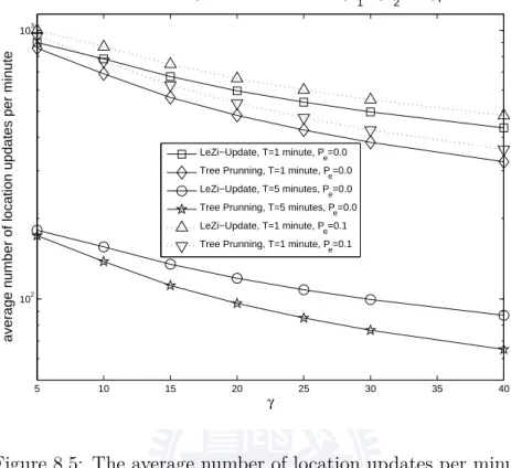
8.5 The average number of location updates per minute . . . 35
Symbols
M: the total number of MTC devices. α: the total number of M2M location areas. L: the width of a M2M location area.
(xm(t), ym(t)): the position of the mth MTC device at time t.
Smax: the maximum speed of a MTC device.
T: a positive real number that represents the length of time slot.
Xk(m): a random variable that represents the index of the M2M location
area in which the mth MTC device resides at time k· T.
G = (V, E): a graph such that each vertex corresponds to a M2M location
area and (i, j)∈ E if and only if there exists a MTC device that might move
from the ith M2M location area to the jth M2M location area in one time
slot.
N1(i) ={j|(i, j) ∈ E}: the adjacent vertices of vertex i.
∆ =min{(2⌈SmaxT
L ⌉ + 1) 2, α}.
d(i, j): the distance between vertex iand vertex j in the graph G. Xk: an abbreviation of X
(m)
k , when only one MTC device is taken into
consideration.
si: the ith substring in the encoding dictionary for the proposed location
update algorithm.
vi: the (maximal proper) prefix ofsi.
wi: the last symbol of si.
f (i): an integer such that sf (i)= vi.
Li: the label of node iin the parsing tree.
Φi: the set composed of the indexes of the children of nodeiin the parsing
tree.
N (t): the total number of nodes in the parsing tree at time t.
tk = k× T: the time instance when a MTC device performs sensing for
the kth time.
Sk: the index of the node that is pointed by the current state pointer just
before time tk.
Θk: a set that is composed of the labels of the children of node (with
index) Sk in the parsing tree.
Γ: a parsing tree.
Γ−k: the tree obtained by removing each node with index greater than k
from the tree Γ.
Φ−k(i): a set that is composed of the indexes of the children of node i in
the tree Γ−k.
{Y−k
n }∞n=0: a discrete-time Markov chain that is associated with the tree
Γ−k.
qi: the estimated value of the probability that the MTC device will appear
in the ith M2M location area.
qi,j: the estimated value of the probability that the MTC device will be
in the jth M2M location area at the next sensing time instance given that
the MTC device is currently in the ith M2M location area.
τ: the index of the M2M location area in which the MTC device currently
resides.
H−k =min{n : n ≥ 1, Yn−k =−1|Y0−k = 0}.
Yn: an abbreviation forYn−k, when the value of k is fixed.
zi =E[min{n : n ≥ 1, Yn=−1}|Y0 = i]. In addition, z = (z0, z1, ..zk)T.
U: a (k + 1)× (k + 1) matrix such that [U]i+1,j+1 = P{Yn+1 = j|Yn = i},
∀0 ≤ i, j ≤ k.
cost and unitary energy cost, respectively.
k∗=arg mink:k∈{0,1,2,..,γ−2}c1× (k + 1) − c2× E[H−k].
Λ(i): a set that is composed of the indexes of M2M location areas that
are adjacent to the ith M2M location area.
ρm: the probability that the mth MTC device will stay in the current
M2M location area after one time slot.
βm: the probability that the mobility pattern of the mth MTC device is
Chapter 1
Introduction
Machine-to-Machine(M2M) communications represents a future where billions of everyday objects and the surrounding environment are connected and managed through a variety of devices, communications networks, and cloud-based servers [9]. Representative M2M usage models include (but are not limited to) smart electric grids, connected cars that react in real time to prevent accidents, and body area networks that track vital signs. M2M communications is a key enabling technology for Internet of Things [10] in which the large number involved leads to a number of research challenges. In 3GPP standards, M2M communication is also called Machine-Type Com-munications (MTC) [11] [12] [13].
In this thesis, we propose an energy-and-memory efficient location update scheme for wireless M2M communications. In particular, we study the case in which the MTC server has to track the location of each MTC device but does not know the mobility patterns of MTC devices in advance. Since it is widely expected that a variety of wireless access networks will coexist in the near future, the proposed location update scheme is designed to be independent of the wireless access networks. In addition to the identity of the closet base station, a MTC device could inform the MTC server its geographical location if the MTC device is equipped with a GPS receiver. Since the total number of MTC devices is expected to exceed the human population, it is desired to
optimize the location update cost for each MTC device.
Novel information-theoretic approaches for location update in wireless cellular networks can be found in [4] [14] [15]. In particular, instead of performing location updates periodically, information theory (source coding theory) [16] is used to decide the optimal time instances for a mobile device to perform location updates. The realizations of the information-theoretic approaches are based on parsing trees. Our major technical contributions include the following. First, based on the theory of random walks over trees [2], we propose a novel algorithm to optimally prune the parsing tree when-ever appropriate. Note that the size of a parsing tree grows with time but the memory size of a MTC device is finite and may not be as large as a smart phone. The proposed algorithm is designed to minimize the weighted sum of the memory cost and the energy cost. In addition, we formally prove that when the weight for the energy cost is smaller than the weight for the mem-ory cost, whenever the parsing tree has to pruned, it is optimal to remove all nodes except the root node. In contrast, when the ratio of the weight for the energy cost to the weight for the memory cost is large enough, it might not be optimal to remove all nodes except the root node. We use both analytical results and simulation results to justify the usage of the proposed approach. The rest of the thesis is organized as follows. Related works are covered in Chapter 2. In Chapter 3, we present the system models and briefly introduce the parsing tree for the benefits of the readers. In Chapter 4, we propose a novel approach to optimally prune the parsing tree based on the theory of random walks over trees. In Chapter 5, we analyze the computational complexity of an algorithm that is used to estimate the location transition probabilities. In Chapter 6, we prove related mathematical results. In Chap-ter 7, we derive the worst-case computational complexity for the proposed location update scheme. In Chapter 8, we show simulation results that reveal the advantages of using the proposed scheme. Our conclusions are included in Chapter 9.
Chapter 2
Related Works
Wireless M2M communications is a young research field. Lopez, Moura, Moreno, and Almeida [17] proposed a M2M-based platform that enables saving energy by remotely monitoring, controlling, and coordinating power generation and consumption in electric grid. Chen and Wang [18] considered optimizations for M2M communications in LTE-A systems. Lien and Chen [19] proposed a massive access management scheme to provide guarantees for MTC devices. In [20], a non-cooperative game-theoretic approach is proposed for distributed rate and admission control in home M2M networks.
In cellular networks, by sensing the signal strengths and listening to broadcast messages, a mobile device could know the identity of the closest base station. Location update and paging are key components for idle-mode mobility management. On the other hand, handover/handoff is essential for connected-mode mobility management. A lot of prior works on paging could be found in the reference of [21] [22]. We focus on location update for a large number of MTC devices in this thesis. Location update schemes could be movement-based [23], timer-based [24], distance-based [25], profile-based [26], state-based [27], or velocity-based [28]. Hybrid location update schemes can be found in [29] and reference therein. Liang and Haas [30] proposed a pre-dictive distance-based user-tracking scheme based on the Markov-Gaussian random process. Cayirci and Akyildiz [31] proposed the user mobility pattern
scheme for location update and paging. Wu, Mukherjee, and Bhargava [32] examined a location update/paging scheme in hierarchical cellular networks. Ng and Chan [33] proposed an enhanced distance-based location management scheme using cell coordinates.
Some researchers assumed that a mobile user sends a location update mes-sage to the system whenever it enters a new location area and concentrated on the design of an optimal location area [14] [34] [35] [36]. Other researchers assumed that location areas are given and focused on the decision problem of whether a mobile user should send a location update message when it enters a new location area [37]. Some proposed location update schemes [38] sug-gested that a mobile user should register its location only when it enters some predefined cells, referred to as reporting centers. In [39], overlapping location areas were proposed to reduce the location update cost. The problem of joint optimization of location update and paging has been investigated in [40] [41]. Jeon and Jeong [42] proposed changing the location update probability of a mobile user based on its call arrival rate and location area change rate. Mao and Douligeris [43] proposed buffering location update messages until a call arrives.
In this thesis, we explicitly take the memory constraints of MTC devices into consideration. Instead of random walks over a graph with cycles, our work is based on the theory of random walks over tree. To the best of our knowledge, the latter is not used in the previous works on location update.
Chapter 3
System Model and The Parsing
Tree
3.1 System Models
In Figure 3.1, we show our network model. In particular, there is a MTC server and M MTC devices, which are indexed by 1, 2, 3, ..., M. The
MTC server is connected to the Internet. On the other hand, a MTC device connects to the Internet through 3G/LTE wireless networks or WiFi access points. The service region of M2M communications is partitioned into α≥ 2
M2M location areas, indexed by 1, 2, 3, ..., α. When each MTC device has a
GPS receiver, a M2M location area corresponds to a square with width equals toLmeters on Earth’s surface. Otherwise, a M2M location area corresponds
to the area covered by a 3G/LTE base station or a WiFi access point. To simplify the descriptions, in this thesis, it is assumes that a MTC device is equipped with a GPS receiver. With minor revisions, the proposed algorithm could be used when a MTC device is not equipped with GPS receiver. It is assumed that whenever a MTC device performs sensing, the MTC device knows the index of the M2M location area in which it currently resides.
Internet
MTC Server WiFi Access Points 3G/LTE Networks MTC Devices MTC Devices GPS SatellitesFigure 3.1: The system model for wireless M2M communications For modeling the mobility of MTC devices, we first introduce a very gen-eral continuous-time model. Next, we create a discrete-time model that is based on the continuous-time model and is sufficient for studying location updates. Let (xm(t), ym(t)) be the position of the mth MTC device at time
t, where tis a non-negative real number. It is assumed that for each integer m, where1≤ m ≤ M, xm(t)and ym(t)are both continuous and differentiable
functions. Let Smax be a positive real number. The maximum speed of a
MTC device isSmaxmeters per second. Recall that location update is a
mech-anism for idle-mode mobility management. In particular, to reduce energy consumption, a mobile device only performs location update occasionally. Thus, we propose the following discrete-time mobility model.
LetT be a positive real number. Time is partition into time slots of equal
length. The length of a time slot equals T seconds. The time interval [(k− 1)T, kT ] is called the kth time slot,∀k ≥ 1. Based on the above
continuous-time mobility model, for the ith MTC device in time slot k + 1, where 1 ≤
−SmaxT ≤ yi((k + 1)T )− yi(kT ) ≤ SmaxT. Let Xk(m) be a random variable
that represents the index of the M2M location area in which the mth MTC
device resides at time kT, ∀k ≥ 0. In order to obtain the value of Xm(m), at
time kT, the mth MTC device performs sensing. A graphG = (V, E), where V is the vertex set andE is the edge set [1], is used to represent the relations
between Xk+1m and Xkm. In particular, vertex i corresponds to the ith M2M
location area, ∀i. Note that (i, j) is the edge between vertex i and vertex j
in the graph G. In addition, (i, j) ∈ E if and only if there exists a pair of
integers (m, k) such that P{Xk+1(m) = j|Xk(m) = i} > 0. Namely, (i, j) ∈ E if
and only if there exists a MTC device that might move from the ith M2M
location area to the jth location area in one time slot. For each i∈ V, define N1(i) ={j|(i, j) ∈ E}.
Denote the cardinality of a set S by|S|. Since the maximum distance of
movement in a time slot for a MTC device isSmaxT and the width of a M2M
location area is L, |N1(i)| ≤ (2⌈SmaxL T⌉ + 1)2. In addition, |N1(i)| ≤ |V | = α.
Thus, |N1(i)| ≤ min{(2⌈SmaxLT⌉ + 1)2, α}. Namely, given that a MTC device is
in theith M2M location area at timekT, we can conclude that at time(k+1)T
the MTC device has to reside in a M2M location area which is indexed by j,
wherej∈ N1(i). While a MTC device might continuously move, for studying
location updates, it is sufficient to use the above discrete-time model. Define
∆ = min{(2⌈SmaxT
L ⌉ + 1)2, α}. Define d(i, j) as the distance between vertex i
an vertex j in the graph G. In particular,d(i, j) is the total number of edges
that belong to the shortest path between vertex iand vertex j in the graph
G.
It is assumed that for each fixed m, the discrete-time stochastic
pro-cess {X(m)
k }∞k=0 is a discrete-time Markov chain (DTMC)[2] with state space
{1, 2, 3, ..., α}. To the best of our knowledge, DTMC is widely used for modeling mobility. Note that if (i, j) /∈ E, P{Xk+1(m) = j|Xk(m) = i} = 0,
∀m, k. A MTC device is either static or mobile. If the mth MTC device
limk→∞P{Xk(m) = j}, ∀m, j. The above DTMC model is very general and
covers a number of mobility patterns. For example, when the movements of the mth MTC device from a random walk or a random walk with drift, {X(m)
k }∞k=0 is a DTMC.
All MTC devices adopt the same location update algorithm and each MTC device runs the location update algorithm independently. Therefore, it is sufficient to consider a MTC device. In the rest of the thesis, when it is clear from the context, we abbreviateXk(m),P{Xk+1(m) = j|Xk(m)= i}, andvj(m)byXk,
P{Xk+1= j|Xk = i}, andvj, respectively. Definepi,j = P{X (m) k+1= j|X
(m) k = i},
∀i, j.
3.2
Parsing Trees for Information-Theoretic
Location Update
A string is composed of a number of symbols. The maximal proper prefix of a string is obtained by removing the last symbol from the string. Among the prefixed of a string, we focus only on the maximal proper prefix of the string. In this thesis, prefix is simply an abbreviation for maximum proper prefix. Note that for a string containing a unique symbol, the prefix is
∅. Denote the concatenation of two strings Y1 and Y2 by Y1 ⊕ Y2, which is
abbreviated by Y1Y2. For example, when Y1 = 12 and Y2 = 345, Y1Y2 =
Y1⊕ Y2 = 12345. Define s0 =∅. For each string s, there exists k substrings
s1, s2, ..., sk (k is an integer k≥ 1) , and a function f such that s = s1⊕ s2⊕
...⊕ sk, f (i) ∈ {0, 1, 2, ..., i − 1}, ∀i ∈ {1, 2, 3, ..., k}, and the prefix of si equals
sf (i), ∀i ∈ {1, 2, 3, ..., k} [3] [4]. Denote the last symbol of si by wi. Denote
the prefix of si by vi. Note that sf (i) = vi and si = vi ⊕ wi. Given a string
s, we can use a parsing tree to find the value of k, the function f, and the
The MTC device maintains a parsing tree and a queue, which is initially empty. A parsing tree is a well-known data structure in the field of source coding [4] [5]. Let γ be the maximum number of nodes in a parsing tree due
to memory constraints. Each node in the parsing tree has an index and a label. In particular, the index of a node is defined to be the order that the node is added into the parsing tree. Note that nodei is the node with index
equal to i. Let Li be the label of node i. In particular, Li is the index of the
M2M location area in which the MTC device resides when node i is added
into the parsing tree. In addition, each node in a parsing tree contains an array of α pointers. Each pointer either points to a child of the node or is
a null pointer. Let Φi be the set composed of the indexes of the children of
node iin the parsing tree.
Initially, the parsing tree is composed of the root node with index zero and label∅. LetN (t)be the total number of nodes in the parsing tree at time t. LetN (t−)be the total number of nodes in the parsing tree just before time
t. If a new node is added into the parsing tree at time t, the index of this
node is set to be N (t−). A MTC device maintains two pointers, which are
called rootandcurrent state, respectively. The root pointer always points to
the root node of the parsing tree. At time zero, the current state pointer also points to the root node of the parsing tree. Definetk= kT,∀k ≥ 1. LetSk be
the index of the node that is pointed by the current state pointer just before time tk, ∀k ≥ 1. Note that S1 = 0. Define Θk = {Lj : j ∈ Φ(Sk)}. Namely,
the set Θk is composed of the labels of the children of nodeSk in the parsing
tree.
At time tk, the value of Xk is inserted into the queue. If Xk ∈ Θk, the
MTC device does not perform location updates. In this case, Sk+1 is set
to be the integer j such that j ∈ Φ(Sk) and Lj = Xk. On the other hand, if
Xk∈ Θ/ k, a new node with indexN (t−k)and labelXkis added into the parsing
tree as a child of node Sk, and then Sk+1 is set to be 0. In addition, based
0, ϕ
1, 1 3, 3 4, 2
2, 2 6, 1 5, 1
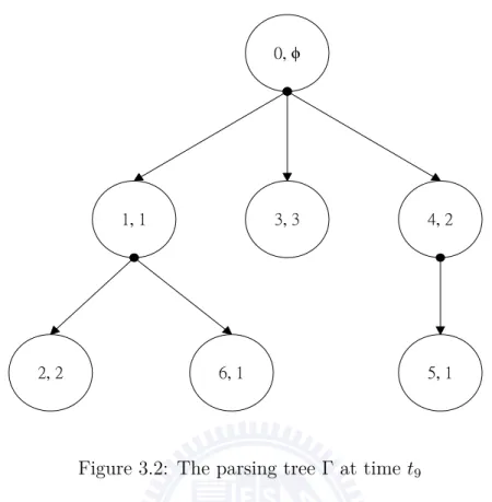
Figure 3.2: The parsing tree Γ at time t9
messages in the queue (into bits) and then clears the queue. In particular, when the kth node is added into the parsing tree, ⌈log2(α· k)⌉ bits are used
to encode all messages in the buffer. In this case, the MTC device performs a location update and sends the bits to the MTC server.
We use the following example to illustrate the above notations. Suppose
α = 4, X1 = 1, X2 = 1, X3 = 2, X4 = 3, X5 = 2, X6 = 2, X7 = 1, X8 = 1,
and X9 = 1. At timet1, since S1 = 0, Φ(S1) =∅, Θ1 =∅, and X1 ∈ Θ/ 1, node
N (t−1) = 1 is added into the parsing tree as a child of node 0 and S2 is set to
be 0. In addition, according to the LZ78 data compression algorithm, we can compute the interger mi = f (i)α + wi− 1, which is the encoded value of X1.
After that, mi is encoded into log2(α· 1) = 2 bits 00. Furthermore, the MTC
device performs a location update and sends the two bits 00 to the MTC server. When the MTC server receives the first location update message form the MTC device, based on the LZ78 data compression algorithm, it decodes the two bits 00 and finds that X1 = 1.
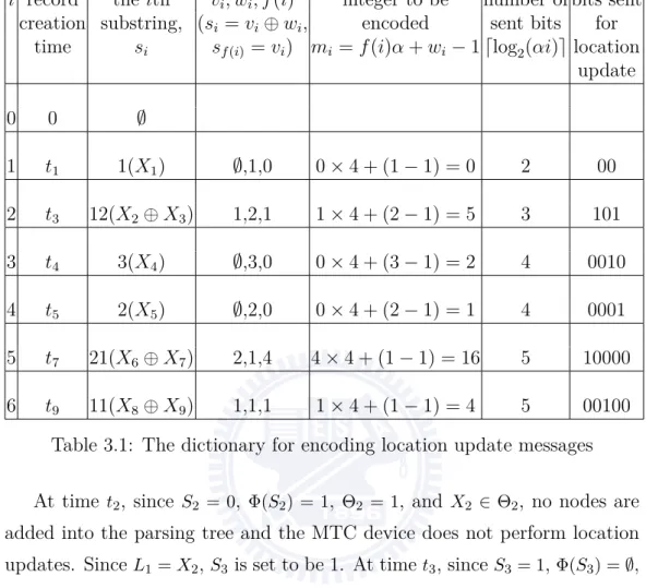
i record the ith vi, wi, f (i) integer to be number of bits sent
creation substring, (si = vi⊕ wi, encoded sent bits for
time si sf (i)= vi) mi = f (i)α + wi− 1 ⌈log2(αi)⌉ location
update 0 0 ∅ 1 t1 1(X1) ∅,1,0 0× 4 + (1 − 1) = 0 2 00 2 t3 12(X2⊕ X3) 1,2,1 1× 4 + (2 − 1) = 5 3 101 3 t4 3(X4) ∅,3,0 0× 4 + (3 − 1) = 2 4 0010 4 t5 2(X5) ∅,2,0 0× 4 + (2 − 1) = 1 4 0001 5 t7 21(X6⊕ X7) 2,1,4 4× 4 + (1 − 1) = 16 5 10000 6 t9 11(X8⊕ X9) 1,1,1 1× 4 + (1 − 1) = 4 5 00100
Table 3.1: The dictionary for encoding location update messages At time t2, since S2 = 0, Φ(S2) = 1, Θ2 = 1, and X2 ∈ Θ2, no nodes are
added into the parsing tree and the MTC device does not perform location updates. SinceL1 = X2,S3 is set to be 1. At timet3, sinceS3 = 1, Φ(S3) =∅,
Θ3 = ∅, and X3 ∈ Θ/ 3, node N (t−3) = 2 is added into the parsing tree as a
child of node 1 and S4 is set to be 0. In addition, according to the LZ78
data compression algorithm, the string X2⊕ X3 = 1⊕ 2 = 12 is encoded into
log2(α· 2) = 3 bits 101. Furthermore, the MTC device performs a location
update and sends the tree bits 101 to the MTC server. When the MTC server receives the second location update message from the MTC device, it decodes the three bits 101 and concludes that(X2, X3) = (1, 2). In Figure 3.2,
we show the corresponding parsing tree at time t9. For each node in Figure
3.2, the first symbol is the index of the node, while the second symbol is the label of the node.
i record expected received received qi, the ri, the si, the ith
creation number bits for integer quotient remainder substring time of bits location mi of dividing of dividing si = sqi⊕ (ri+ 1)
⌈log2(αi)⌉ update mi by α mi by α
0 0 1 t1 2 00 0 0 0 ∅ ⊕ (0 + 1) = 1 2 t3 3 101 5 1 1 1⊕ (1 + 1) = 12 3 t4 4 0010 2 0 2 ∅ ⊕ (2 + 1) = 3 4 t5 4 0001 1 0 1 ∅ ⊕ (1 + 1) = 2 5 t7 5 10000 16 4 0 2⊕ (0 + 1) = 21 6 t9 5 00100 4 1 0 1⊕ (0 + 1) = 11
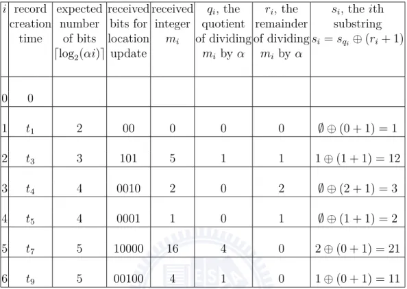
Table 3.2: The dictionary for decoding location update messages
In Table 3.1, we show the dictionary used by the MTC device for com-pressing location update messages into bits at time t9, when the LZ78
algo-rithm is used. In table 3.2, we also show the corresponding dictionary used by the MTC server for decompressing received bits at time t9.
Note that MTC device performs location updates only when new nodes are added into the associated parsing tree. Therefore, the location update cost is reduced. In addition, since the above approach of location update corresponds to a lossless data compression scheme [3], the MTC server knows all values of Xk’s [4].
We include pseudo codes for maintaining the parsing tree in Algorithm 1. In particular, some of the pseudo codes use the syntax of the C programming language.
Algorithm 1: The Parsing Tree Formation Algorithm
1 //initialize the parsing tree 2 if initialization then
3 parsingTree.root = (struct treeNode *)malloc(sizeof(struct
treeNode));
4 parsingTree.root→ index = 0; //the index of the root node is 0 5 parsingTree.root→ label = -1; //the label of the root node is ∅ 6 parsingTree.root→ totalChildren = 0; //the total number of
children of the root node
7 parsingTree.root→ childNode = (struct treeNode
**)malloc(totalBaseStation*sizeof(struct treeNode *));
8 parsingTree.currentNode = parsingTree.root; //current state
pointer
9 parsingTree.nextId = 1; //index for the next node added into the
parsing tree
10 //update the parsing tree when obtaining the kth sensing result, Xk 11 if getNewSensingResult(k) then
12 add Xk into the tail of the queue;
13 if Xk ∈ Θk then
14 //does not perform location updates or add new nodes into the
parsing tree
15 j = findChildIndex(Xk,Φ(Sk)); //find j such that j ∈ Φ(Sk)
and Lj = Xk;
16 parsingTree.currentNode = node j in the parsing tree;
//update the current state pointer
17 else
18 //add a new node into the parsing tree
19 totalChildren = parsingTree.currentNode.totalChildren; 20 parsingTree.currentNode.child[totalChildren] = (struct
treeNode *)malloc(sizeof(struct treeNode));
21 parsingTree.currentNode.child[totalChildren].index = parsingTree.nextId; 22 parsingTree.currentNode.child[totalChildren].label = Xk; 23 parsingTree.currentNode.totalChildren++; 24 parsingTree.currentNode = parsingTree.root; parsingTree.nextId++;
25 //perform a location update
Chapter 4
Optimally Pruning The Tree
In this chapter, based on the theory of random walks over trees, we pro-pose a novel approach to optimally prune the parsing tree. For each MTC device, the memory size is finite and therefore the parsing tree connot keep growing forever. Whenever it it necessary to prune the parsing tree, it is desired to prune the parsing tree in an optimal way so that the cost is min-imized. In addition, both the memory cost and the energy cost should be taken into consideration. Typically, memory cost is an increasing function of the total number of nodes in the parsing tree. On the other hand, the en-ergy cost is a decreasing function of the expected value of the time difference between two consecutive location updates. We will explicitly define the cost function later in this chapter.
4.1 Constuct The DTMC for The Tree Γ
−kSuppose now we have to prune the parsing tree Γ. Namely, there are γ
nodes in the parsing tree we have to remove at least one node from the tree
Γ. To maintain the structure of the parsing tree for decompression, if node
i is removed and i < j, node j also has to be removed. Let Γ−k be the tree
obtained by removing each node with index greater than k from the tree Γ.
node. Let Φ−k(i) be the set composed of the indexes of the children of node
i in the tree Γ−k.
Given that the parsing tree Γ is currently pruned to be Γ−k, we can
predict the next location update time based on the movement history of the MTC device. In particular, for the tree Γ−k, we construct the associated
discrete-time Markov chain{Y−k
n }∞n=0with state spaceΩ−k ={−1, 0, 1, 2, ..., k}
as follows. First, state iof the DTMC corresponds to nodeiin the treeΓ−k,
∀0 ≤ i ≤ k. In addition, state -1 is an absorption state. In particular, given that Y0−k = 0, Ym−k =−1 if and only if the MTC device performs a location
update at timetm. The state transition probabilities of the DTMC{Yn−k}∞n=0
should depend on the mobility pattern of the MTC device.
In order to set the state transition probabilities for the DTMC{Y−k n }∞n=0,
we first define a few variables. Letqibe the estimated value of the probability
that the MTC device will appear in the ith M2M location area. Let qi,j be
the estimated value of the probability that the MTC device will be in the
jth M2M location area at the next sensing time given that the MTC device
is currently in the ith M2M location area. These values can be iteratively
computed when every time the MTC device reports its location information. Later in the thesis, we will present an algorithm to derive the values of qi
and qi,j. It is desired to set P{Yn+1 = j|Yn = i} = P {Xn+1 = Lj|Xn = Li},
∀1 ≤ i, j ≤ k. However, the value of P{Xn+1 = Lj|Xn = Li} is not always
known in advance. Therefore, whenever the value of P{Xn+1 = Lj|Xn= Li}
is required, we use the value ofqLi,Lj instead. Letτ be the index of the M2M location area in which the MTC device currently resides. We propose setting the state transition probabilities for the DTMC {Y−k
P{Yn+1−k = j|Yn−k = i} = qτ,Lj, if i = 0 and j ∈ Φ−k(i) 1−∑j:j∈Φ−k(i)qτ,Lj, if i = 0 and j =−1 qLi,Lj, if 1≤ i ≤ k and j ∈ Φ−k(i) 1−∑j:j∈Φ−k(i)qLi,Lj, if 1≤ i ≤ k and j = −1 1, if i = j =−1 0, otherwise.
We now elaborate on the above equation. Suppose the current state pointer points to the node with index i. Denote the next sensing result by s.
If i = 0, the MTC device resides in the τth M2M location area. In this case,
if s∈ {Lj|j ∈ Φ−k(i)}, the MTC device will not perform a location update
when it will get the next sensing result. Instead, the current state pointer will point to the node with index equalsj, wherejis and integer such thatLj = s.
Given that the MTC device is in the τth M2M location area, the probability
that the next sensing result will be s equals pτ,s. Since the value of pτ,s is
not known in advance, if i = 0 and j ∈ Φ−k(i), we set P{Yn+1−k = j|Yn−k = i}
to be pτ,Lj. If i = 0 and s /∈ {Lj|j ∈ Φ−k(i)}, the MTC device will perform a location update when it will get the next sensing result. Therefore, we set P{Yn+1−k =−1|Yn−k = 0} = 1 −∑j:j∈Φ
−k(i)qτ,Lj. If i≥ 1, the MTC device resides in the Lith M2M location area. Similar to the case in which i = 0, if
i≥ 1 and j ∈ Φ−k(i), we set P{Yn+1−k = j|Yn−k = i} be qLi,Lj. In addition, we setP{Yn+1−k =−1|Yn−k = i} to be1−∑j:j∈Φ
−k(i)qLi,Lj. The state -1 is designed to be and absorption state. Therefore, P{Yn+1−k =−1|Yn−k =−1} = 1.
We use the following example to illustrate the above notations. Suppose
α = 4, X1 = 1, X2 = 1, X3 = 2, X4 = 3, X5 = 2, X6 = 2, X7 = 1, X8 = 1, and
X9 = 1. Suppose we want to prune the tree at time t9. Then, τ = X9 = 1.
Based on the estimation algorithm in Chapter 5, at time t9, we have q1 = 59,
0 1 3 2 -1 3/4 0 1/4 1/4 3/4 1 1 1
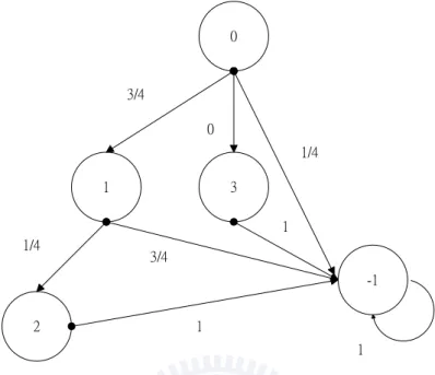
Figure 4.1: The state transition diagram for the DTMC associated with Γ−3 at time t9
Figure 3.2, we have showed the parsing tree Γ at time 9. In Figure 4.1, we
show the state transition diagram for the DTMC corresponding to Γ−3 (at
time t9). Except for the state -1, a state of the DTMC {Yn−3}∞n=0 in Figure
4.1 corresponds to the index of a node of the tree in Figure 3.2. For example, since the node with index 1 and label 1 is a child of node 0 and q1,1 = 34,
we have P{Yn+1−3 = 1|Yn−3 = 0} = 43. In addition, P{Yn+1−3 = −1|Yn−3 = 0} = 1− q1,1− q1,3 = 14. Similarly, since the node with index 2 and label 2 is a
child of node 1 and q1,2= 14, we haveP{Yn+1−3 = 2|Yn−3 = 1} = 14. Furthermore,
P{Yn+1−3 =−1|Yn−3 = 1} = 1 − q1,2 = 34. Moreover, due to that node 3 is a leaf
node in Γ−3, P{Yn+1−3 =−1|Yn−3= 3} = 1 − 0 = 1.
4.2
Optimal Solution for Pruning The Tree
LetH−k be a random variable that represents the time instance when the
discrete-time Markov chain {Y−k
that Y0−k = 0. In particular,
H−k =min{n : n ≥ 1, Yn−k =−1|Y0−k = 0}. (4.1)
Note that the DTMC {Y−k
n }∞n=0 corresponds to a random walk over the tree
Γ−k. In addition, the random variable H−k corresponds to the length of the
time interval elapsed from now to the time instance when the MTC device performs the next location update, given that the current parsing tree isΓ−k
and the current state pointer points to the root node. The larger the value of
H−k is, the longer waiting time that MTC device needs to make next location
update. Thus, the smaller the energy cost for location update is.
We now derive the value of E[H−k]. Consider a fixed value of k. To
simplify the notations, we abbreviate Yn−k by Yn. Define zi =E[min{n : n ≥
1, Yn = −1}|Y0 = i]. Namely, zi is the average number of steps it takes for
the DTMC {Yn}∞n=0 to visit state -1 for the first time, given that Y0 = i. In
particular, z0=E[H−k]. Then, based on [2], ∀i ∈ {0, 1, 2, ..., k},
zi = 1 + k
∑
j=0
P{Yn+1= j|Yn= i} × zj. (4.2)
We now elaborate on the above equation. First, it takes at least one step for the DTMC {Yn}∞n=0 to move from state i to state -1, ∀i ̸= −1. Given that
Y0 = i, with probability P{Yn+1 = j|Yn= i}, Y1 = j. For each j ̸= −1, given
that Y1 = j, on average, it takes zj additional steps for the DTMC {Yn}∞n=0
to move from state j to state -1. Therefore, we have the above equation.
Letz = (z0, z1, ..., zk)T and 1k+1 = (1, 1, ..., 1)T be two (k + 1)-dimensional
column vectors. Define a (k + 1)× (k + 1) matrix U such that [U]i+1,j+1 =
P{Yn+1= j|Yn= i},∀0 ≤ i, j ≤ k. For the above example, which is associated
U = 0 34 0 14 0 0 14 0 0 0 0 0 0 0 0 0 . (4.3)
Recall that for a parsing tree, the index of a node corresponds to the order that the node is inserted into the parsing tree. Thus, that node j is a
child of node iimpliesj > i. Therefore, U is an upper triangular matrix and
[U]i,i = 0, ∀i. Then, based on Equation (4.2), we have the following matrix
equation:
z = 1k+1+U× z. (4.4)
Let Ik+1 be the (k + 1)th order identity matrix. Then,
(Ik+1− U) × z = 1k+1. (4.5)
Based on the Gauss elimination method, the above equation can be solved inO(k3) time. We now show that the above matrix equation can be solved in
O(k)time. SinceUis an upper triangular matrix,(Ik+1−U)is also an upper-triangular matrix. In addition,[Ik+1−U]i,i= 1,∀i. Thus, the matrixIk+1−U
is full-ranked. Since the matrix (Ik+1 − U) is both upper-triangular and
full-ranked, Equation (4.5) can be solved by backward substitution without explicitly calculating the inverse matrix (Ik+1− U)−1. Recall that when the
graph G = (V, E) represents a tree, |E| = |V | − 1 [1]. Since there are k + 1
nodes andkedges in the treeΓ−k, there areknonzero elements in the matrix
Uandk + (k + 1) = 2k + 1 nonzero elements in the matrixIk+1−U. Therefore,
Letc1, c2 > 0 be two real numbers. Denote the optimal value ofk byk∗.
We propose using the following approach to find the value of k∗.
k∗=arg min
k:k∈{0,1,2,...,γ−2}{c1× (k + 1) − c2× E[H−k]}.
(4.6)
Note that c1× (k + 1) corresponds to the memory cost, since there are (k+1)
nodes in the parsing tree Γ−k. On the other hand, −c2× E[H−k]corresponds
to the energy cost. The larger the average length of the interval between two time instances of performing location updates is, the smaller the energy cost is.
Once the value of k∗ is obtained, the MTC device prunes the parsing
tree Γ such that nodes with indexes greater than k∗ are removed from the
parsing tree. In addition, the current state pointer points to the root node of the parsing tree. Furthermore, the MTC device informs the MTC server the latest value of k∗.
The proposed tree pruning algorithm and the encoding algorithm are executed in each MTC device in a distributed manner, while the decoding algorithm is executed in the MTC server (or Gateway) in a centralized man-ner. For location update, there are no control message exchanges between MTC devices. When the total number of MTC devices is very large, a cluster of MTC servers could be used for load balancing.
Chapter 5
Estimating The Location
Transition Probabilities
For the completeness of the thesis, we now present an algorithm for es-timating the location transition probabilities of a MTC device. The algo-rithm is quite simple and its variants have been widely used. Let qm,i be
the estimated value of the probability that the MTC device will appear in the ith M2M location area at the next sensing time based on the values of X1, X2, ..., Xm. Let qm,i,j be the estimated value of the probability that the
MTC device will appear in the jth M2M location area at the next sensing
time given that the MTC device is currently in the ith M2M location area,
based on the values of X1, X2, ..., Xm. Let I(condition) be the indicator
func-tion with value one if the condifunc-tion is true or with value zero otherwise. To reduce the memory requirement, during the time interval[tm, tm+1), the MTC
device only keeps the values of Xm, qm−1,i’s, qm,i’s, and qm,i,j’s. Thus, the
space requirement of the estimation algorithm is O(1 + α + α + α2) = O(α2).
values of qm+1,i’s according to the following equation: qm+1,i = ∑m+1 k=1 I(Xk= i) m + 1 = ∑m k=1I(Xk= i) + I(Xm+1 = i) m + 1 = m· qm,i m + 1 + I(Xm+1 = i) m + 1 ,∀i. (5.1)
In addition, at timetm+1, the MTC device calculates the values ofqm+1,i,j’s
as follows. First, if ∑m
k=1I(Xk = i) = 0, qm+1,i,j = 0, ∀j. On the other hand,
if ∑m k=1I(Xk= i)≥ 1, qm+1,i,j = ∑m k=1∑I(Xk= i, Xk+1 = j) m k=1I(Xk= i) = ∑m 1 k=1I(Xk= i)· [ m∑−1 k=1 I(Xk= i, Xk+1= j) +I(Xm = i, Xm+1= j)] = 1
m· qm,i · [(m − 1) · qm−1,i· qm,i,j
+I(Xm = i, Xm+1= j)],∀j. (5.2)
The computational complexity of Equation (5.1) for calculation the value ofqm,i’s isO(α). In addition, the computational complexity of Equation (5.2)
for calculating the values of qm,i,j’s is O(α2). Therefore, the computational
complexity of the estimation algorithm is O(α + α2) = O(α2).
If at timetm, the MTC device has to purne the parsing tree, the value of
qi in Chapter 4 is set to be the value of qm,i. In addition, the value of qi,j in
Chapter 6
Analytical Results
Consider a MTC device. LetVnbe a random variable that represents the
nth time when the parsing tree has γ nodes (then the MTC device needs to
prune the parsing tree), ∀n ≥ 1. We first prove that the random variable V1
is finite for sure (with probability one). From the time instance when the current state pointer points to the root node to the time instance when a new node is added into the parsing tree, each of the old nodes in the parsing tree is pointed by the current state pointer in at most one sensing period. Therefore, it takes at most k sensing periods for the total number of nodes
in the parsing tree to increase from k to k + 1. Hence, V1 ≤
∑γ−1 k=1k =
γ(γ−1) 2
for sure. In worst case, if we find out that optimal value k∗ = γ− 2, the next
time when the parsing tree hasγ nodes equals toV1. Thus,Vn+1−Vn≤ γ(γ2−1)
for sure, ∀n ≥ 1.
Consider a parsing treeΓthat containsγ nodes. We now derive properties
for the random variables H−k’s. First, H−0 = 1 for sure. Since Γ−k is a
tree that contains no cycles, starting from state 0, the DTMC {Y−k n }∞n=0
never visits state i twice before it visits the state -1, ∀1 ≤ i ≤ k. Thus, the
DTMC {Y−k
n }∞n=0 visits up to k state before it visits the state -1. Therefore,
H−k ≤ k + 1 for sure. Furthermore, it can be proved that 1 < E[H−1] <
Let Zn be a random variable that represents the state of the parsing
tree at time Vn, ∀n ≥ 1. Let W (t) be the total number of nodes in the
parsing tree at time t. By definition of Vn, W (Vn) = γ, ∀n ≥ 1. Let ΩZ
be the state space of the random variables Zn’s. Define ζ = |ΩZ|. We now
prove that ζ ≤ [(α + 1) × (γ!α!)]γ < ∞. First, there are γ nodes in the
parsing tree at time Vn, ∀n ≥ 1. For a node in the parsing tree, the total
number of children ranges from 0 toα. When a node hasm≥ 1 children, the
total number of combinations for the indexes of the m children is at most γ× (γ − 1) × ... × (γ − m + 1), which is no greater thanγ!. When a node has m = 0 children, the total number of combinations for the indexes of the m
children is 1, which is also smaller than γ!.
Similarly, when a node hasm≥ 1 children, the total number of
combina-tions for the labels of the m children is at mostα× (α − 1) × ... × (α − m + 1),
which is no greater than α!. When a node has m = 0 children, the total
number of combinations for the label s of the m children is 1, which is also
smaller than α!. Therefore, ζ ≤ [(α + 1) × (γ!α!)]γ <∞. Sinceζ <∞, for each
realization of the stochastic process {Zk}ζ+1k=1, denoted by {Zk(ω)}
ζ+1
k=1, there
exists two integers G1(ω) and G2(ω) such that
1≤ G1(ω) < G2(ω)≤ ζ + 1 (6.1)
Ifc2
c1 is small enough, whenever the parsing tree has to pruned, it is optimal
to remove all nodes except the root node.
Lemma 1: If c2
c1 < 1, k
∗= 0.
Proof:
1. Define f (k) = c1 · (k + 1) − c2· E[H−k], ∀k ∈ {0, 1, 2, .., γ − 2}. Then,
f (0) = c1− c2. 2. Whenk≥ 1, f (k) ≥ c1(k + 1)− c2(k + 1) = (c1− c2)(k + 1) > c1− c2 = f (0).
SinceH−k ≤ k +1 for sure,E[H−k]≤ k +1. Thus, we have the first inequality.
Since c1, c2 > 0 and cc21 < 1, c1− c2 > 0. In addition, k + 1 > 1, ∀k ≥ 1. Thus,
we have the third inequality.
3. Since f (0) < f (k), ∀k ≥ 1, k∗=arg min0≤k≤γ−2f (k) = 0.
QED.
In contrast, if c2
c1 is large enough, it might not be optimal to remove all
nodes except the root node.
Lemma 2: If there exists an integer j, where j ∈ Φ0 and j ̸= γ − 1, such
that c2· qτ,Lj − c1· j > 0, k∗ ≥ 1.
Proof:
1. Define f (k) = c1 · (k + 1) − c2· E[H−k], ∀k ∈ {0, 1, 2, .., γ − 2}. Then,
f (0) = c1− c2.
2. E[H−j]≥ 1 + qτ,Lj. Thus, f (j)≤ c1(j + 1)− c2(1 + qτ,Lj). 4. f (0)− f(j) ≥ c2· qτ,Lj − c1· j > 0.
5. Thus,k∗̸= 0 and therefore k∗ ≥ 1.
The following theorem provides a sufficient condition for the DTMC
{Zn}∞n=1 to be irreducible, aperiodic, and positive-recurrent.
Theorem 1: If qi = vi, ∀i, qi,j = P{Xk+1 = j|Xk = i}, ∀i, j, cc21 < 1,
γ > α,the DTMC {Xk}∞k=1 is irreducible, and P{Xk+1 = i|Xk = i} > 0,
∀1 ≤ i ≤ α, then the DTMC {Zn}∞n=1 is irreducible,aperiodic, and
positive-recurrent.
Proof:
1. We first prove that the DTMC is irreducible. Let ξ1, ξ2 ∈ ΩZ be two
distinct states. Consider the case in whichZ1 = ξ1. Sinceξ1 ∈ ΩZ, there exists
an integer θ1 ∈ {1, 2, 3, .., α} such that given that X0 = θ1, with probability
greater than zero, Z1 = ξ1. Similarly, there exists an integer θ2 ∈ {1, 2, 3, .., α}
such that given that X0 = θ2, with probability greater than zero, Z1 = ξ2.
2. At time V1, the parsing tree is pruned and only the root node is kept
based on Lemma 1. Recall that d(i, j) is the total number of edges on the
shortest path from vertexito vertexjin the graphG. DefineN1= d(XV1, θ2).
Since the DTMC {Xk}∞k=1 is irreducible, with probability greater than zero,
XV1+N1 = θ2. Since d(XV1, θ2) < αfor sure and α < γ− 1,N1 < γ− 1 for sure.
Due to that N1< γ−1and at most one node is added into the parsing tree in
a sensing period,V2 > V1+N1 for sure. SinceP{Xk+1= θ2|Xk= θ2} > 0, given
that XV1+N1 = θ2, with probability greater than zero, XV1+N1 = XV1+N1+1 =
.. = XV2 = θ2.
3. At time V2, the parsing tree is pruned and only the root node is kept
based on Lemma 1. In addition, based on the definition of θ2, given that
XV2 = θ2, with probability greater than zero, Z3= ξ2.
4. Based on 2 and 3, P{Z3 = ξ2|Z1 = ξ1} > 0 and therefore the DTMC is
irreducible.
5. We now prove that the DTMC is aperiodic by showing that P{Z3 =
ξ1|Z1 = ξ1} > 0 and P{Z4 = ξ1|Z1 = ξ1} > 0. Consider the case in which
Z1 = ξ1. At time V1, the parsing tree is pruned and only the root node is
greater than zero, XV2 = θ1.
6. At time V2, the parsing tree is pruned and only the root node is kept
based on Lemma 1. In addition, based on the definition of θ1, given that
XV2 = θ1, with probability greater than zero, Z3= ξ1.
7. Based on 5 and 6,P{Z3 = ξ1|Z1 = ξ1} > 0.
8. We now prove thatP{Z4 = ξ1|Z1 = ξ1} > 0. At timeV1, the parsing tree
is pruned and only the root node is kept based on Lemma 1. SinceP{Xk+1=
i|Xk= i} > 0, ∀i, with probability greater than zero, XV1 = XV1+1 = .. = XV2.
9. Similar to 5, given thatXV2 = XV1, with probability greater than zero,
XV3 = θ1. Similar to 6, given that XV3 = θ1, with probability greater than
zero, Z4 = ξ1.
10. Based on 8 and 9,P{Z4 = ξ1|Z1 = ξ1} > 0
11. Based on 7 and 10, due to that the greatest common divisor of
3−1 = 2and 4−1 = 3is 1, the period of the stateξ1 is one. Since the DTMC
is irreducible, all states have the same period and therefore the DTMC is aperiodic.
12. Since |ΩZ| < ∞, the DTMC has at least one positive-recurrent state.
Since the DTMC is irreducible and has at least one positive-recurrent state, all states are positive-recurrent.
QED.
If qi = vi,∀i, qi,j = P{Xk+1 = j|Xk = i}, ∀i, j, cc21 < 1, γ > α, the DTMC
{Xk}∞k=1 is irreducible, and P{Xk+1 = i|Xk = i} > 0, ∀1 ≤ i ≤ α, based on
the above theorem, limn→∞P{Zn = ξ|Z1 = ξ1} exists and is independent of
ξ1, ∀ξ, ξ1 ∈ ΩZ. In this case, the DTMC {Zn}∞n=1 has a unique steady-state
Chapter 7
Complexity Analysis
In this chapter, for the proposed location update algorithm, we analyze the worst-case computational complexity in time and space. Recall that
∆ =min{(2⌈SmaxT
L ⌉ + 1)2, α} and |N1(i)| ≤ ∆,∀i ∈ V. Consider a MTC device
in a time slot.
We now analyze the time complexity. First, it takes at most O(∆) time
to check if a new node should be added into the parsing tree in the current time slot. If a new node should be added, it takes O(1) time to add the
new node. Otherwise, it takes O(1)time to update the current state pointer.
Second, as shown in Chapter 4, it takes O(k) time to calculate the value of
E[H−k], ∀0 ≤ k ≤ γ − 2. Thus, it takes at most O(∑γk=0−2k) = O(γ2) time to
obtain the value of k∗. Recall that ∆≤ α, and as shown in Chapter 5, the
time complexity for estimating the location transition probabilities is O(α2).
Therefore, the time complexity of the proposed location update scheme is upper bounded by
We now analyze the space/memory complexity. First, there are at mostγ
nodes in the parsing tree. Thus, it takes⌈log2(γ)⌉ bits to represent the index
of a node in the parsing tree. Second, since there are α M2M location areas
in the network, it takes ⌈log2(α)⌉ bits to represent the label of a node in the
parsing tree. Third, a node in the parsing tree has at most∆children. Recall
that the space complexity for estimating the location transition probabilities is O(α2). Therefore, the space complexity of the proposed location update
algorithm is upper bounded by
Chapter 8
Simulation Results
We wrote C programs in Windows 7 to obtain discrete event-driven simu-lation results [6] [7]. Each simusimu-lation instance consists of 100,000 time slots. We study the case in which the service region is a square and is partitioned intoα = w2 M2M location areas of equal size. LetΛ(i)be the set composed of
the indexes of M2M location areas that are adjacent to theith M2M location
area. Note that |Λ(i)| ∈ {2, 3, 4}. For a MTC device in a time slot, the mem-ory cost equals the total number of nodes in the parsing tree multiplied by the value of c1. On the other hand, for a MTC device, the total energy cost
equals the total number of location updates performed by the MTC device during the simulated time interval multiplied by the value ofc2. For a MTC
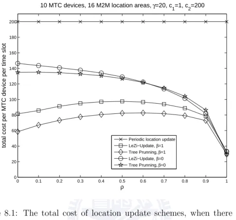
device in a simulation instance, the total cost is defined to be the sum of the total memory cost and the total energy cost, such like Equation (4.6).
We evaluate the proposed tree pruning algorithm, the LeZi-Update al-gorithm [4], and the naive periodic location update alal-gorithm. When the LeZi-Update is used and it is necessary to prune the parsing tree, except for the root node, all nodes of the parsing tree are deleted. For a MTC device, when the naive periodic location update scheme is used, the memory cost per time slot is zero and the energy cost per location update equals c2, regardless
of the mobility pattern. As in many previous works on location update, it is assumed that the wireless channel is characterized byPe, the probability that
0 0.1 0.2 0.3 0.4 0.5 0.6 0.7 0.8 0.9 1 0 20 40 60 80 100 120 140 160 180 200 ρ
total cost per MTC device per time slot
10 MTC devices, 16 M2M location areas, γ=20, c1=1, c2=200
Periodic location update LeZi−Update, β=1 Tree Prunning, β=1 LeZi−Update, β=0 Tree Prunning, β=0
Figure 8.1: The total cost of location update schemes, when there are 10 MTC devices
a location update message is not successfully received by the access point/ base station. Unless explicitly stated, Pe = 0 in this chapter.
We use the following DTMC-based mobility model in the C programs. A MTC device is either static or mobile. The movements of two mobile MTC devices are statistically independent. It is assumed that for each m, {X(m)
k }∞k=0 is a DTMC and X (m)
0 is an integer-valued random variable that
is uniformly distributed in [1, α]. After one time slot, a mobile MTC device
either stays in the current M2M location area or moves to one of the adjacent M2M location areas.
To model a variety of mobility patterns, the DTMC-based mobility model has three parameters, ρm, βm, and h. ρm is the probability that the mth
mobile device will stay in the current M2M location area after one time slot.
βmis the probability that the mth MTC device moves along a predetermined
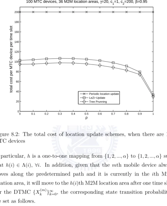
0 0.1 0.2 0.3 0.4 0.5 0.6 0.7 0.8 0.9 1 0 20 40 60 80 100 120 140 160 180 200 ρ
total cost per MTC device per time slot
100 MTC devices, 36 M2M location areas, γ=20, c1=1, c2=200, β=0.95
Periodic location update LeZi−Update Tree Prunning
Figure 8.2: The total cost of location update schemes, when there are 100 MTC devices
In particular, h is a one-to-one mapping from {1, 2, ..., α} to {1, 2, ..., α}such
that h(i) ∈ Λ(i), ∀i. In addition, given that the mth mobile device always
moves along the predetermined path and it is currently in the ith M2M
location area, it will move to theh(i)th M2M location area after one time slot.
For the DTMC {X(m)
k }∞k=0, the corresponding state transition probabilities
are set as follows.
P{Xk+1(m) = j|Xk(m) = i} = ρm, if j = i (1− ρm)(βm+ 1|Λ(i)|−βm), if j = h(i)
(1− ρm)(1|Λ(i)|−βm), if j ∈ Λ(i) − {h(i)}
0, otherwise.
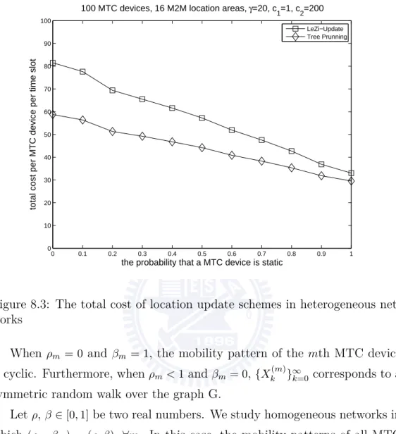
0 0.1 0.2 0.3 0.4 0.5 0.6 0.7 0.8 0.9 1 0 10 20 30 40 50 60 70 80 90 100
the probability that a MTC device is static
total cost per MTC device per time slot
100 MTC devices, 16 M2M location areas, γ=20, c1=1, c2=200
LeZi−Update Tree Prunning
Figure 8.3: The total cost of location update schemes in heterogeneous net-works
When ρm = 0 and βm = 1, the mobility pattern of the mth MTC device
is cyclic. Furthermore, when ρm< 1 and βm= 0,{Xk(m)}∞k=0 corresponds to a
symmetric random walk over the graph G.
Letρ,β ∈ [0, 1]be two real numbers. We study homogeneous networks in
which (ρm, βm) = (ρ, β), ∀m. In this case, the mobility patterns of all MTC
devices are identical. In Figure 8.1, we show the total cost per MTC device per time slot, When M = 10, α = 16, and β∈ {0, 1}. In comparison with the
naive periodic location update scheme, the proposed location update scheme could reduce the total cost by at least 32%. When the movement pattern of each MTC device is cyclic, regardless of the value ofρ, the proposed location
update scheme outperforms the LeZi-Update algorithm. In particular, the reduction in the total cost ranges from 7% to 28%. When the mobility pattern of each mobile device is cyclic, the proposed location update algorithm could use a small parsing tree to correctly predict the movements of a mobile
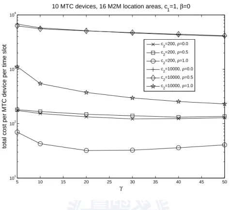
5 10 15 20 25 30 35 40 45 50 101 102 103 104 γ
total cost per MTC device per time slot
10 MTC devices, 16 M2M location areas, c1=1, β=0
c 2=200, ρ=0.0 c 2=200, ρ=0.5 c 2=200, ρ=1.0 c 2=10000, ρ=0.0 c 2=10000, ρ=0.5 c 2=10000, ρ=1.0
Figure 8.4: The impacts of the maximum number of nodes in a parsing tree device and reduce the frequency of location update. Therefore, in terms of the overall cost, the proposed location update algorithm outperforms the LeZi-Update algorithm. When the movements of each MTC device form a symmetric random walk andρ < 0.6, the proposed location update algorithm
is superior to the LeZi-Update algorithm. When the movements of each MTC device form a symmetric random walk and ρ > 0.6, the proposed location
update algorithm is slightly inferior to the LeZi-Update algorithm.
In Figure 8.2, we show the total cost per MTC device per time slot, when M = 100, α = 36, and β = 0.95. In this case, regardless of the value
of ρ, the proposed location update algorithm outperforms the LeZi-Update
algorithm. In comparison with the periodic location update scheme, the proposed location update algorithm could reduce the total cost by at least 50%. In comparison with the LeZi-Update algorithm, the proposed location update algorithm could reduce the total cost by up to 10%.