國 立 交 通 大 學
電信工程學系碩士班
碩 士 論 文
多天線頻域正交多工系統之
頻率,資料與通道的合併估測
Joint Frequency, Data and Channel Estimation
for MIMO OFDM Systems
研究生:呂子逸
指導教授:蘇育德 博士
ӭϺጕᓎୱ҅Ҭӭπسϐ!
ᓎ-ၗᆶ೯ၰޑӝٳෳ!
Joint Frequency, Data and Channel Estimation
for MIMO OFDM Systems
ࣴ!ز!ғǺֈηຽ!!!
!
!
!
!
Student : Tzu-I Lu
ࡰᏤ௲Ǻػቺ!റγ
Advisor
:
Dr.
Yu
T.
Su
!
୯!ҥ!Ҭ!೯!ε!Ꮲ!
ႝߞπำᏢسᅺγ!
ᅺ!γ!ፕ!Ў!
!
A Thesis Submitted to
Department of Communications Engineering
College of Electrical Engineering and Computer Science
National Chiao Tung University
In Partial Fulfillment of the Requirements
For the Degree of Master of Science
In
Communications Engineering
July 2005!
Itjodiv-!Ubjxbo-!Sfqvcjd!pg!Dijob!
!
ӭϺጕᓎୱ҅Ҭӭπسϐ!
ᓎ-ၗᆶ೯ၰޑӝٳෳ!
ࣴزғǺֈηຽ!
!!! !
!
!
!
!
ࡰᏤ௲Ǻػቺ!റγ!
୯ҥҬ೯εᏢႝߞπำᏢسᅺγ!
!
ᄔा!
ךॺӧᓎୱ҅Ҭӭπ(OFDM)سύӝٳᓎǵၗᆶ೯ၰޑෳޑё Չ܄Ƕҗܭၩݢᓎୃ౽(Carrier Frequency Offset, CFO)܌ԋޑᓎୱߞဦޑၩ ݢ໔υᘋ(Inter-Carrier Interference, ICI)ᆶፄ৩೯ၰ܌Їଆӧਔ໔ື಄ዸ໔υ ᘋ(Inter-Symbol Interference, ISI)Ԗᜪ՟ޑኧᏢኳԄǴࡕޣޑӭςޕှ،БਢǴ ӵനεёૈ܄ׇӈෳ(Maximum Likelihood Sequence Estimation, MLSE)Ǵߡё Ҕٰှ،ޣǶฅԶǴόӕܭޑ MLSE ёޔௗҔ Viterbi ᄽᆉݤǴךॺय़ ჹޑࢂ֖Ԗ҂ޕୖኧȐόዴۓ܄ȑޑ(Trellis)კǶךॺ௦ҔሀԄӝٳᔠ ෳᆶी(Iterative Joint Detection and Estimation)ޑচ߾ٰှ،Ƕ२ӃǴךॺଞჹൂϺጕ (SISO) سޑރݩٰीǴ٠ЪଞჹਏૈϷፄᚇࡋ ЬाፐᚒගрׯБਢǶךॺፕΑճҔௗԏᆄຎื(Windowing)ޑਏᘠݢ Ϸմନၨλၩݢυᘋޑᎃᓎफ़եރᄊ(trellis state)ኧҞޑБݤޑёՉ܄а फ़եᄽᆉݤޑፄᚇࡋǶךॺΨ௦Ҕόӕ೯ၰෳݤჹسਏૈޑቹៜǶௗ Ǵךॺஒ೭ሀԄӝٳᔠෳᆶीᄽᆉݤډӭϺጕ(MIMO)ޑسǶ ࣁࣴزךॺ܌ගрᄽᆉݤޑਏૈϷӚسϷ೯ၰୖኧޑਏǴךॺ௦ڗ IEEE802.11nྗǴTask Group‘n’synchronizationȐ܈ᙁᆀ TGn Syncȑ܌ගрٰ ޑᒡߞဦࢎᄬࣁ୷ᘵٰႝတኳᔕǶ܌ளډޑኧॶ่݀ᡉҢǴคፕࢂ SISO ܈
Joint Frequency, Data and Channel Estimation for
MIMO OFDM Systems
Student : Tzu-I Lu Advisor : Yu T. Su
Department of Communications Engineering National Chiao Tung University
Abstract
We consider the problem of joint carrier frequency offset (CFO)/channel estimation and data detection for orthogonal frequency-division multiplexing (OFDM) systems. An iterative approach is employed. The iteration procedure consists of an inner CFO/data estimation loop and an outer CFO/data-channel estimation loop. We first discuss the single-input single-output (SISO) case and then extend to a input multiple-output (MIMO) scenario. Drawing an analogy between the inter-carrier interference corrupted frequency domain waveform and the inter-symbol interference limited time domain waveform, we apply maximum likelihood sequence estimation scheme to detect the data sequence in the presence of residual CFO. Related algorithms either for reducing the implementation complexity like the trellis state number or for improving the overall performance such as receiver time domain windowing and refined channel estimates are presented. Computer simulation results based on a candidate IEEE 802.11n standard– the Tgn Sync (Task Group n) proposal–are given to predict the performance of the proposed algorithms.
ᇞᖴ!
!
ࣴز܌ޑٿԃύǴߚதགᖴךޑࡰᏤ௲ǺػቺԴৣǶӧдൻ
ൻ๓ᇨޑ௲ᏤύǴ٬ךૈӦஒҁፕЎֹԋǶࣴزޑၸำ
ύǴഋࡏדᏢߏаϷࢫ٫։ӕᏢόս๏ϒཱུεޑᔅշǹᏢۂ
ॺ׳ޑᜅշႝတሺᏔаٮኳᔕϐҔǴзךӳғགǶ!
ӧЈޑፓᆶࡌǴζ϶ࢋ➌Ǵӳ϶γ◖ǵࡹᓪܭѳਔջό
ᘐޑႴᓰךǴ٠ЪፓᏊךޑғࢲ፪ǴᡣךᏱԖᑈཱུӛޑΚໆа
ၸࣴزύޑᓍǶੇၖЦฝΨࢂךᓸޑБԄϐǴЬفᎹ०ޑኾ
Κ׳ࢂךനӳޑڂጄǶ!
ԜѦǴձགᖴᖄวࣽמϦљޑᜅշаϷࡰᏤǴ٬ளࣁයԃޑ
ࣴزीฝளаճՉǶനࡕǴჹךޑР҆ᒃаϷৎΓठΜϩޑᖴ
ཀǴགᖴдॺ๏ϒךؼӳޑᕉნǴᡣךޑᏢғఱคࡕ៝ϐኁǶ!
Contents
English Abstract i
Contents ii
List of Figures v
1 Introduction 1
2 Joint Frequency Data and Channel Estimation for SISO-OFDM
Sys-tems 5
2.1 Joint CFO Estimation and Data Detection . . . 5
2.1.1 System model in AWGN channels . . . 5
2.1.2 Joint frequency-data sequence estimation algorithm . . . 8
2.1.2.1 Data detection . . . 8
2.1.2.2 CFO estimation . . . 9
2.2 Joint Estimator for Frequency-Selective Channels . . . 11
2.2.1 System model for frequency-selective channels . . . 11
2.2.2 Joint frequency-data sequence-channel (FDC) estimation algorithm 12 2.2.2.1 Channel estimation . . . 12
2.3 Numerical Experiments . . . 15
3 Further Study on the Detecting SISO-OFDM Signals 19 3.1 Receiver Window Design . . . 19
3.1.1 Double-length FFT and square windowing . . . 20
3.1.2 Adaptive Nyquist windowing . . . 22
3.1.2.1 “Folding” method . . . 28
3.1.3 Effect of windowing on ICI and noise Power . . . 30
3.1.3.1 ICI Analysis . . . 30
3.1.3.2 Noise power analysis . . . 33
3.1.4 Complexity issue . . . 34
3.2 Reducing the Number of Trellis States . . . 34
3.2.1 Complexity issue . . . 36
3.3 Channel Estimation . . . 36
3.3.1 Jakes model . . . 36
3.3.2 Model-based channel estimate . . . 38
3.3.3 2D model-based channel estimate with transform-domain process-ing (2-D+TDP) . . . 40
3.3.4 Complexity issue . . . 41
3.4 Numerical Experiments . . . 41
4 Joint Estimation for MIMO-OFDM Systems 45 4.1 Introduction . . . 45
4.2 System Model . . . 46
4.3 MIMO-OFDM Channel Estimation . . . 47
4.4 An Iterative Joint FDC Estimation Algorithm . . . 50
4.5 Numerical Experiments . . . 51
5 Conclusion 54
A 802.11n PHY Specification 55 A.1 MIMO data path overview . . . 55 A.2 High Throughput (HT) PHY layer convergence protocol (PLCP)
pream-ble . . . 56 A.3 Basic MIMO PPDU format . . . 58
List of Figures
2.1 Block diagram of an OFDM modulator. . . 6 2.2 Structure of complete OFDM signal with the guard period (interval). . . 6 2.3 Block diagram of a typical OFDM demodulator. . . 7 2.4 An example of cost value for CFO=0.2 without noise. . . 10 2.5 Illustrating the proposed iterative joint Frequency-Data Sequence-Channel
(FDC) estimation algorithm”. Initially, the switch is in position 1; and for the tracking mode it is moved to position 2; It stops when the new channel estimation is close enough to the previous estimate . . . 14 2.6 BER performance of SISO-OFDM systems using iterative joint FD
esti-mate in AWGN channels with different fe. . . 16 2.7 MSEE performance of CFO estimates for the joint FD estimate in AWGN
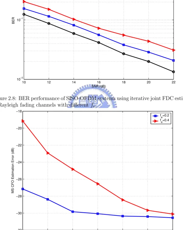
channels. . . 16 2.8 BER performance of SISO-OFDM systems using iterative joint FDC
es-timate in Rayleigh fading channels with different fe. . . 17 2.9 MSEE performance of CFO estimates for the joint FDC estimate in
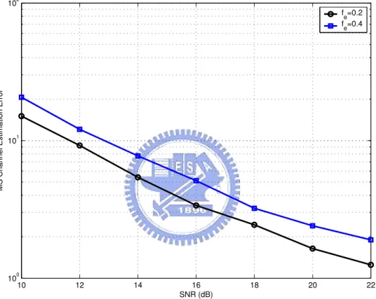
Rayleigh fading channels. . . 17 2.10 MS channel estimation error of the joint FDC estimate in a Rayleigh
fading as a function of fe. . . 18
3.1 Double length of OFDM-symbol(a)time domain, (b)2N rectangular win-dow, (c)frequency domain. . . 21 3.2 Filter bank and the placement of the N carriers . . . 22
3.3 Completed OFDM-symbol (a)time domain, (b)Nyquist window, (c)frequency
domain. . . 23
3.4 The time functions of raised-cosine pulse, and BTRC pulse with different α. . . 24
3.5 Raised cosine window and BTRC window depending of roll-off factor α . 26 3.6 DFT-filter bank with Nyquist windowing (α = 0) . . . 26
3.7 Graphical representation of a 8-FFT . . . 27
3.8 Folding of the receiver window. . . 29
3.9 Comparison of ICI power for different baseband pulse-shaping functions (α = 0.1) in a 64-subcarrier OFDM system. . . 32
3.10 ICI power associated with different base pulse-shaping functions (α = 1) in a 64-subcarrier OFDM system. . . 32
3.11 SIR for different baseband pulse-shaping functions (α = 0.1) in a 64-subcarrier OFDM system. . . 33
3.12 Power percentage distribution of BTRC in frequency domain for each subcarrier at CFO = 0.2. . . 35
3.13 Ray arrival angles in the Jakes model (N = 10). . . 37
3.14 Real part of a Jakes fading process. . . 38
3.15 Regression of LS channel under SNR=12dB. . . 40
3.16 A complete channel estimation process. . . 40
3.17 BER performance of SISO-OFDM systems using iterative joint FD esti-mate with different windowing in AWGN channels. . . 43
3.18 BER performance of SISO-OFDM systems using iterative joint FDC es-timate with different windowing in Rayleigh fading channels. . . 43
3.19 Effect of channel estimate on the SISO-OFDM system’s BER performance. 44 3.20 BER performance of SISO-OFDM systems using iterative joint FDC es-timate with reduced-state DF method in Rayleigh fading channels. . . 44
4.1 Channel model for the qth receive antenna. . . 48
4.2 BER performance of MIMO- and SISO-OFDM systems using iterative joint FDC estimate (fe = 0.2). . . 52
4.3 MSEE performance of CFO estimates in MIMO-OFDM systems for 2 × 2 and SISO configurations (fe = 0.2). . . 52
4.4 Effect of the channel estimate on the MIMO-OFDM system’s BER per-formance (fe = 0.2). . . 53
A.1 The MIMO datapath of the IEEE 802.11n standard. . . 55
A.2 HT Preamble format . . . 57
Chapter 1
Introduction
The main idea behind the orthogonal frequency division multiplexing (OFDM) wave-form is to split a data block into multiple parallel sub-blocks so that each of them is transmitted by distinct orthogonal subcarriers. The orthogonality between those trans-mitted sub-streams is ensured by choosing a proper subcarrier spacing. By inserting a cyclic prefix in the (parallel-to-serial) combined time-domain signal before it is transmit-ted via the main carrier, intersymbol interference (ISI) caused by a multipath channel can be eliminated at the receiving end if the corresponding cyclic prefix part in each OFDM frame is removed.
The cyclic prefix (also known as the guard interval) of an OFDM block is a copy of the last portion of the original block and if the maximum channel path delay is smaller than the guard interval duration, the received time-domain waveform will be a weighted sum of various delayed version of the transmitted blocks. Deleting the cyclic prefix, each data-bearing subcarrier experiences only flat fading. Such an arrangement enables an OFDM-based system to overcome frequency selective fading in broadband wireless transmission and is the major reason for its current popularity.
Due to its effectiveness, OFDM has been selected as standards for various wireless applications, such as digital audio broadcasting (DAB) [1], digital video broadcasting (DVB) [2]-[4], high performance local area networks (HIPERLAND/2) [5], and IEEE
802.11a wireless local area networks (WLAN) [6]. OFDM also plays an important role in future standards, such as IEEE 802.11n [7] [8], 802.16e, and 802.20, some of them are likely to include the Multiple Input Multiple Output (MIMO) option for capacity enhancement. We will give a brief introduction in Section A.
With all its merits, OFDM, unfortunately, is far more sensitive to synchronization errors, especially the carrier frequency offset (CFO), than single carrier systems. CFO is primarily caused by relative movement or channel-induced Doppler shifts and in-stabilities of and mismatch between transmitter and receiver oscillators [9]. In high dynamic environment, the received waveform is likely to encounter large Doppler shifts by antipodal frequencies. Residual CFO results in inter-carrier interference (ICI) among subcarriers due to the loss of orthogonality and will bring about serious performance degradation. Whence it is highly desirable to reduce the sensitivity of OFDM systems to CFO of any kind.
There have been a multitude of proposals for CFO compensation. But most of them require pilot symbols or training sequences [10], which lowers the effective data rate. Blind techniques that operate in the time domain [11] often require observation over a number of OFDM symbols, and are not suitable for tracking time-varying CFO. Decision-directed modifications of some pilot-assisted CFO estimation are more promis-ing but require good initial estimate. On the other hand, the ultimate goal of a receiver is the detection of the transmitted data stream and, as the detection of OFDM signals takes place in the frequency domain, channel estimation must be obtained before data detection commences. Conventional OFDM channel estimators, however, are derived under a zero or negligible CFO assumption. We therefore face the dilemma of chan-nel estimation in the presence of CFO and CFO estimation without pilots or reliable decisions.
It is thus the goal of this investigation to develop feasible solutions to the above joint estimation and detection problem. We adopt an iterative approach for joint
CFO/channel estimation, tracking and data detection. To simply our problem, we shall assume that the initial CFO is to be less than one half of the subcarrier spacing. Draw-ing an analogy between the ICI effect on a frequency domain signal and the ISI effect on a time domain signal, we can easily apply the maximum likelihood sequence estimation (MLSE) technique to detect the data stream in the presence of ICI, assuming known CFO.
Chapter 2 begins with the simple scenario that no channel estimation is needed. Assuming an initial CFO estimate we use the Viterbi algorithm to obtain an estimate of the transmitted data sequence. The CFO estimate is then refined and updated by considering the new information provided by the estimated data sequence. The updated CFO, in turn, is used to modify the trellis for a new run of Viterbi detection. The iteration procedure stops when convergence is achieved (usually 2 or 3 iterations is enough).
When frequency selective fading is present, channel estimate is needed for data detec-tion. Because the channel estimation requires CFO information our iterative procedure will consist of two loops in which the joint CFO/data estimation constitute an inner loop while the joint channel and CFO/data estimation procedure forms the outer loop. More specifically, the inner loop follows the same iterative procedure described in the above paragraph and, when a convergence is detected, the information is passed to the channel estimator to produce a new estimate. The new channel estimate is then used by the inner loop for another run of joint CFO/data estimation. Simulation results indicate that both inner and outer loops converge very rapidly. The complexity is mostly associ-ated with the Viterbi search and channel estimator. The former has to do with the ICI range, i.e., the number of neighboring subcarriers that interfere the desired subcarrier while the latter depends on the algorithm used.
In Chapter 3, we suggest the use of Nyquist windowing in time domain to suppress the ICI effect and reduce the number of trellis states through truncation and decision
feedback [22]. We also study the effectiveness of an improved channel estimator. It is shown that the receiver complexity is greatly reduced without significant performance degradation.
Chapter 4 extends our investigation to a MIMO environment and finally, Chapter 5 summarizes the main results and suggests topics for further studies. In all simulations, BPSK is used as the subcarrier modulation. For reference purpose, we provide a brief description of the IEEE 802.11n standard proposed by the TGn Sync group in Appendix A.
Chapter 2
Joint Frequency Data and Channel
Estimation for SISO-OFDM
Systems
In a real-world scenario, received OFDM signals often suffer from residual frequency offsets, caused by oscillator instabilities and relative movement-induced Doppler spread, resulting in inter-carrier interference (ICI) among subcarriers. It is desirable to reduce the sensitivity of OFDM to carrier frequency offsets .
2.1
Joint CFO Estimation and Data Detection
2.1.1
System model in AWGN channels
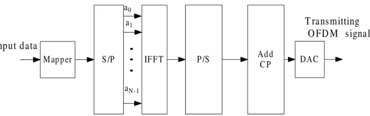
Shown in Fig. 2.1 is a block diagram of an OFDM transmitter. The mapper converts input data stream into complex valued constellation points, according to the selected constellation, e.g., BPSK, QAM. The complex valued data sequence is parallel-to-serial converted before being used to modulate multiple carriers via an inverse discrete Fourier transformation (usually through the inverse fast Fourier transform, IFFT).
Each OFDM symbol has a “useful interval” of length Tu and a cyclic prefix (CP)(or “guard interval”) with duration Tg; see Fig. 2.2. The CP is a periodical repetition of the useful interval so that precise timing recovery is not needed as long as the discrete Fourier transform frame of the receiver starts within the guard interval. In order to protect the
T ransmitting O FD M signal
a0
Mapper S/P IFFT P/S AddC P DAC
a1
aN-1
Input data
Figure 2.1: Block diagram of an OFDM modulator.
OFDM signal against inter-symbol interference (ISI), the CP is set longer than the maximum channel memory, Tg/Tu < 0.25 being a practical value. The baseband signal is modulated by a Nyquist signaling pulse, up-converted to the radio frequency (RF) and then transmitted through the channel. At the receiver, the signal is down-converted
s[1] s[2] s[N -1] s[N -1] s[N -G ] Tu has N samples Tghas G samples C omplete O FD M signal
Figure 2.2: Structure of complete OFDM signal with the guard period (interval).
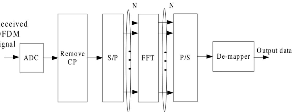
to the intermediate frequency (IF) and then demodulated (Fig. 2.3). After removing the cyclic prefix, the signal part of the received time-domain baseband waveform can be expressed as s[n] = 1 N N −1X k=0 akej2πnk/Nej2πfen/N (2.1) where,
• ak represents the symbol carried by the kth subcarrier. The i.i.d. data sequence {ak} is such that E[ak] = 0 and E[|ak|2] = 1.
R emove
C P S/P
ADC FFT P/S
N N
De-mapper O utput data
Received O FD M signal
Figure 2.3: Block diagram of a typical OFDM demodulator.
• N = the number of subcarriers.
• fe is CFO normalized by the intercarrier spacing ft = 1/Tu and Tu is an OFDM symbol period (without cyclic prefix).
This time domain signal is then passed through a serial-to-parallel convertor and then an FFT demodulator. Assuming an AWGN channel, the signal at the FFT output becomes
rk = 1 N N −1X n=0 s[n]w[n]e−j2πnk/N + n k (2.2)
where w[n] represents the receiver pulse shaping function and nk is additive white Gaus-sian noise (AWGN). Plugging (2.1) into (2.2), the received signal can be written as
rk = N −1X m=0 am ( 1 N N −1X n=0 w[n]e−j2πn(k−m)/Nej2πfen/N ) + nk = X m amWk−mfe + nk = akW0fe + X m6=k amWk−mfe | {z } ICI +nk (2.3) = yk(fe, a) + nk (2.4) where Wfe k = N1 PN −1 n=0 w[n]e−j2πnk/Nej2πfen/N
channel driven by the input a with the channel response Wfe
k ,dependent upon the given CFO, fe. The choice of the window function w[n] affects the extent of ISI (actually the ICI in this case). To control the complexity of the estimator, the length of Wfe
k must be kept reasonably short. We will discuss how to choose pulse shaping function later in Section 3.1.
2.1.2
Joint frequency-data sequence estimation algorithm
With a proper window shaping, we can rewrite (2.3) as rk ≈ akW0fe +
m=k+LX m=k−L,m6=k
amWk−mfe + nk (2.5)
where L is usually less or equal than 2 for |fe| < 0.5 .
2.1.2.1 Data detection
Given ˆfe, the data detection is equivalent to estimating the state of a discrete-time finite-state machine. The finite-state machine in this case is the equivalent discrete-time channel with coefficients {Wfˆe
k } and its state at any instant in time is given by the 2 ∗ L most recent inputs. Even though we have noncausal term in (2.5), we can add a delay function so that the resulting model is causal.
rk−L ≈ akW ˆ fe −L+ ak−1W ˆ fe −L+1+ ... + ak−2LW ˆ fe L + nk−L (2.6)
The state at time k is
Sk = (ak−1, ak−2, ..., ak−2L) (2.7)
If the information symbols are M -ary, the channel filter has M2L states. Consequently, the channel is described by an M2L-state trellis and the Viterbi algorithm may be used to determine the most probable path through the trellis.
2.1.2.2 CFO estimation
Given ˆa as well as r, we can get a CFO estimate by finding fe that minimizes the cost function
C(fe) = X
k
|rk− yk(fe, ˆa)|2 (2.8)
The minimization of (2.8) is carried out base on a gradient descent search method as following: ∇fe(C(fe)) = ∂C ∂fe (2.9) = X k {−A · r∗k− A∗· rk+ B · A∗+ A · B∗}
where ( )∗ denote the complex conjugate and
A = X m am(Wk−mfe )0 ≈ k+L X m=k−L am(Wk−mfe )0 , (Wk−mfe )0 = ∂Wfe k−m ∂fe B = X m amWk−mfe ≈ k+L X m=k−L amWk−mfe (2.10) A learning rate u is introduced to control the rate of change in each iteration
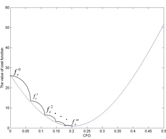
fe1 ← fe0− u ∗ ∇fe(C(f 0 e)) fe2 ← fe1− u ∗ ∇fe(C(f 1 e)) ... fem ← fem−1− u ∗ ∇fe(C(f m−1 e )) When fm
e reaches a stable value with very little jitter, which indicates that we have arrived at a minimum, the algorithm stops; see Fig. 2.4.
1 e f m e
f
0 ef
2 ef
The joint frequency-data sequence (FD) estimation algorithm consists of the follow-ing steps:
A.1 (Frequency Estimate Initialization) Set the initial estimate ˆfe to zero.
A.2 (Starting the FD iteration loop) Using the CFO estimate ˆfe, generate the corre-sponding frequency domain “channel response” Wfe
k : Wfe k = 1 K K−1X n=0 w[n]e−j2πn(k−m)/Kej2πfen/K
A.3 (Compute the tentative data estimate) Based on the observation baseband samples r, we run the Viterbi algorithm using the branch metric
λk= |rk− yk( ˆfe, a)|2
to obtain an estimate ˆa of the transmitted data sequence.
A.4 (Update the frequency estimate) Given ˆa from Step 3 as well as r, we obtain a new CFO estimate by searching for fe that minimizes the cost function
C = X
k
|rk− yk(fe, ˆa)|2
A.5 (Convergence check and end of the FD loop) If the new CFO estimate is close enough to the previous estimate, i.e. absolute difference is less than 10−6, then stop the iteration and release the most recent estimate; otherwise, go to Step 2. Simulation shows that this algorithm usually converges within just two or three itera-tions.
2.2
Joint Estimator for Frequency-Selective
Chan-nels
2.2.1
System model for frequency-selective channels
For frequency-selective fading channels, we assume that the CP is longer than the channel impulse response whence there is no frequency domain self interference between
successive OFDM symbols. With such an assumption we can concentrate on a single OFDM symbol scenario. Let the signal part of the received signal be given by
s[n] = 1 N N −1 X k=0 akHkej2πnk/Nej2πfen/N (2.11)
where Hk is the channel response at k/T . After taking FFT, the received signal becomes
rk = 1 N N −1 X n=0 s[n]w[n]e−j2πnk/N + nk (2.12)
Like the AWGN case, we have rk =
N −1X m=0
amHmWk−mfe + nk
= yk(fe, a, H) + nk (2.13)
2.2.2
Joint frequency-data sequence-channel (FDC) estimation
algorithm
The estimator proposed in the previous section cannot be applied directly to (2.13) because the channel response is unknown. However, assuming the data sequence and the CFO are known, the channel impulse response can be easily estimated.
2.2.2.1 Channel estimation
For every subcarrier n, the channel can be estimated as (using LS): ˆ Hn= 1 an [(FHF)−1FHr]n , n = 0, 1, ..., N − 1 (2.14) where F = Wfe 0 · · · W fe −N +1 ... . .. ... Wfe N −1 · · · W fe 0 r = r0 r1 ... rN −1
Based on this channel estimator and the joint CFO-data sequence estimator proposed in the previous section, we arrive at the following iterative joint CFO-data sequence-channel estimation algorithm.
B.1 (Channel estimate initialization) Let ˆHO to be the channel estimate from the previous OFDM symbol interval.
B.2 (FD iteration loop) Using this channel estimate, the CFO fe and the symbol sequence a are estimated by the joint FD estimation algorithm described in the previous section.
B.3 (Channel estimate update) Compute a new channel estimate ˆHN using (2.14) based on the current estimates ˆfe and ˆa.
B.4 (Convergence check for the channel estimate) If the new channel estimate ˆHN is close enough to the previous estimate, more specifically, if
¯ ¯ ¯ ¯ ¯ ˆ HN − ˆHO ˆ HN ¯ ¯ ¯ ¯ ¯ 2 < 10−2
then stop iteration and release the most recent estimates. If not, go to Step 2. We plot the overall receiver structure in Fig. 2.5.
Rem ove CP S/P AD C FFT P /S N N Received OFDM signal D ata (Viterbi algorithm ) CFO
(G radient descent m ethod)
Channel (LS algorithm ) P revious Hn Initial fe= 0 Channel is close to previous ? CFO is close to previous ? Y es N o Y es N o 1 2 1 2
Figure 2.5: Illustrating the proposed iterative joint Frequency-Data Sequence-Channel (FDC) estimation algorithm”. Initially, the switch is in position 1; and for the tracking mode it is moved to position 2; It stops when the new channel estimation is close enough to the previous estimate .
2.3
Numerical Experiments
The computer simulation results reported in this section are obtained by using a pilot and data format which are the same as the Tgn Sync 802.11n proposal (52 data tones and 4 pilot tones); see the Appendix. It is a slight modification of the IEEE 802.11a data format (48 data tones and 4 pilot tones).
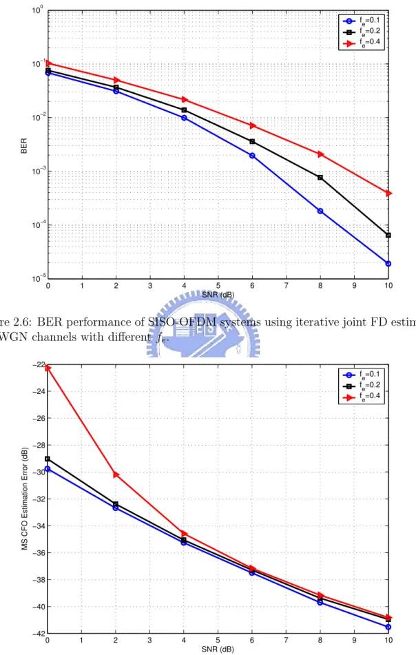
From Fig. 2.6 we can see that the proposed joint FD estimator gives good BER performance in AWGN channels. The mean squared estimation error (MSEE) perfor-mance of the frequency estimate for different fe is plotted in Fig. 2.7, where SNR is defined as the ratio of the total transmit signal energy per bit to noise power density.
The frequency-selective fading channel is modelled as an linear FIR filter with impulse response given by
h(k) = CXL−1
n=0
αne−jΦδ(k − n) (2.15)
where Φ is uniformly distributed in [0, 2π) and αn is Rayleigh distributed with an expo-nential power profile
α2
n= (1 − e−Ts/Trms)e−nTs/Trms.
with CL=10, Trms=30ns and Ts=50ns. We use Jakes channel model with maximum Doppler shift of 500 Hz to simulate time-correlated Rayleigh fading αn.
Fig. 2.8 and Fig. 2.9 present respectively the BER and MSEE performance of the CFO estimator in frequency-selective fading channels. And we show the MSEE of the channel estimator in Fig. 2.10. These performance curves indicate that the BER performance is dominated by the channel estimation error since the MSEE of the CFO estimator is relatively small, especially at high SNRs where the MSEE of our frequency estimate reaches an almost constant floor while the channel estimate’s MSEE continues to decrease.
0 1 2 3 4 5 6 7 8 9 10 10−5 10−4 10−3 10−2 10−1 100 SNR (dB) BER fe=0.1 fe=0.2 fe=0.4
Figure 2.6: BER performance of SISO-OFDM systems using iterative joint FD estimate in AWGN channels with different fe.
0 1 2 3 4 5 6 7 8 9 10 −42 −40 −38 −36 −34 −32 −30 −28 −26 −24 −22 SNR (dB)
MS CFO Estimation Error (dB)
fe=0.1 fe=0.2 fe=0.4
10 12 14 16 18 20 22 10−2 10−1 100 SNR (dB) BER fe=0 fe=0.2 fe=0.4
Figure 2.8: BER performance of SISO-OFDM systems using iterative joint FDC estimate in Rayleigh fading channels with different fe.
10 12 14 16 18 20 22 −32 −30 −28 −26 −24 −22 −20 −18 SNR (dB)
MS CFO Estimation Error (dB)
fe=0.2 fe=0.4
Figure 2.9: MSEE performance of CFO estimates for the joint FDC estimate in Rayleigh fading channels.
10 12 14 16 18 20 22 100
101 102
SNR (dB)
MS Channel Estimation Error
fe=0.2 fe=0.4
Figure 2.10: MS channel estimation error of the joint FDC estimate in a Rayleigh fading as a function of fe.
Chapter 3
Further Study on the Detecting
SISO-OFDM Signals
This chapter presents two modifications on the algorithm discussed in the previous chapter to enhance the BER (bit error rate) performance. We fist show that, with a proper time-domain windowing in place before the DFT operation, we can reduce the ICI due to CFO. Our second improvement is obtained by using a proper model-based channel estimation method. We demonstrate that improved performance is obtained, especially at high SNRs. Since the complexity of the joint estimator is mostly associated with the Viterbi search, we also show the number of trellis states can be reduced when the normalized absolute CFO is small (≤ 0.2).
3.1
Receiver Window Design
As shown in Chapter 2, conventional OFDM reception [13] makes no use of the signal samples in the guard interval (GI) as they might be corrupted by multipath interference. Only the so-called useful (cyclic prefix-removed) samples are retained and sent to the ensuing discrete Fourier transform (DFT) block for further frequency-domain signal processing. This corresponds to a plain rectangular windowing on the received samples in time domain. Muschalik [14] showed that spectral properties improvement is achieved by allowing excess time in the demodulation window. In many channels, the GI is oversized, i.e., the actual channel-impulse response duration is shorter than the
implemented GI. We refer to that part of the GI which is not affected by echoes from previous OFDM symbols as unconsumed GI. Samples in that region can be exploited to improve performance.
The use of windowing on the time-domain samples before the DFT operation (receiver windowing) reduces the side lobe amplitude but also leads to the loss of orthogonality amongst subcarriers. A window which reduces the side lobes while retains the carrier orthogonality is called a Nyquist window. Muschalik [14] first proposed the use of the raised cosine window to suppress ICI in OFDM systems. Tan and Beaulieu [15] then suggest a new window and claimed that it is superior to the raised cosine window in ICI reduction. These windows need a part of the GI that is not affected by echoes and whose length depends on the channel conditions [18]. As its name suggests, receiver windowing is a receiver-only technique, so it is applicable to systems without requiring a change to the transmitter (which is typically the specified part of a standard).
Other approaches to OFDM transmission with modified window shapes [16] [17], include transmitter modifications to reduce out-of-band power of the transmitter by waveform shaping which is different from the receiver-only approach.
3.1.1
Double-length FFT and square windowing
Since in many cases only a portion of the GI is necessary in order to avoid ISI, the other “variable” part of the GI may be used for Nyquist windowing. We first try to use 2N samples in order to maintain the orthogonality.
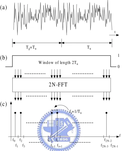
One way to improve the frequency response of the filter bank is to prolong the rectangular window interval to double its length (2Tu) before taking FFT (Fig. 3.1(a)). In this case the GI Tg has to be the same length as the usable interval Tg = Tu and has N samples. So now, an FFT of length 2N rather than of length N has to be performed, as shown in Fig. 3.1(b). Fig. 3.1(c) plots the spectrum of a double length OFDM-symbol. The new filter bank consisting of 2N square windowings and the placement of
Tg=Tu Tu 0 1 W indow of length 2Tu
2N -FFT
f0 f1 f2 fi f2N-2 f3 fi-1 fi+1 fi-2 f2N-1 f2N-3 f t(a)
(b)
(c)
ft=1/TuFigure 3.1: Double length of OFDM-symbol(a)time domain, (b)2N rectangular window, (c)frequency domain.
the N carriers are shown in Fig. 3.2. We can easily see that there is an additional zero crossing between two carriers. Only the odd or even filters of the filter bank contain the carriers and are used to extract the information. The other so called ghost filters contain only disturbances like noise and are not used. Therefore only one half of the 2N FFT coefficients need to be calculated to the end. The advantage of having twice as many filters (2N ) on the filter bank is that the odd or even filters integrate the same carrier power but only one half of the white noise power of the N -filter case for same maxima value. It results in an improvement on carrier to noise ratio C/N of 3 dB.
f
k
ff
k+1
f
k+2
f
k−1
f
k−2
...
...
Figure 3.2: Filter bank and the placement of the N carriers
The disturbance power filtered by the “ghost” filters is the gain of this filter bank. The handicap of this kind of windowing is that we need a very long GI (Tg = Tu). Therefore the 2N square windowing is under normal conditions unrealizable but, as will be shown in the next subsection, it allows the better understanding of the Nyquist windowing.
3.1.2
Adaptive Nyquist windowing
With GI length between 0 and Tu ,i.e. Tu ≥ Tg ≥ 0, the Nyquist windowing may be implemented to improve the frequency response of the DFT filter. In the case of multipath reception only the “usable GI” Tv is used for the windowing. Tv is supposed to be free of ISI. The windowing is adaptive because Tv depends on channel conditions, hence has variable length. Fig. 3.3 shows the way to implement an adaptive Nyquist windowing.
(a)
Tg T
uhas N sam ples
t
Tv has V sam ples
1
(b)
(c)
0 Nyquist window ft=1/Tu2N -FFT
f0 f1 f2 fi f2N-2 f3 fi-1 fi+1 fi-2 f2N-1 f2N-3 fFigure 3.3: Completed OFDM-symbol (a)time domain, (b)Nyquist window, (c)frequency domain.
The usable part of the GI Tv consists of V samples. The V samples of Tv together with the OFDM-symbol Tu (N samples) are symmetrically windowed. The window w(t) has a shape which fulfills the time domain analogy to the Nyquist criterion.
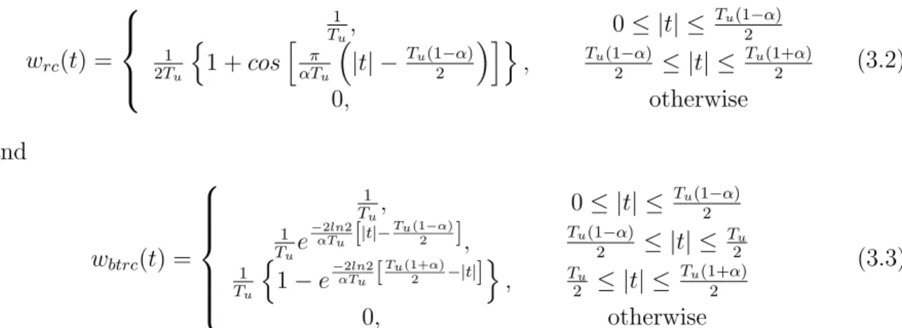
We consider three time-limited pulses. Let wr(t), wrc(t) and wbtrc(t) denote the rectangular pulse, the raised-cosine pulse (in the continuous time domain), and the “better than” raised-cosine (BTRC) pulse (in the time domain) defined as
wr(t) = ½ 1 Tu, − Tu 2 ≤ |t| ≤ Tu 2 0, otherwise (3.1)
wrc(t) = 1 Tu, 0 ≤ |t| ≤ Tu(1−α) 2 1 2Tu n 1 + cosh π αTu ³ |t| − Tu(1−α) 2 ´io , Tu(1−α) 2 ≤ |t| ≤ Tu(1+α) 2 0, otherwise (3.2) and wbtrc(t) = 1 Tu, 0 ≤ |t| ≤ Tu(1−α) 2 1 Tue −2ln2 αTu [|t|−Tu(1−α)2 ], Tu(1−α) 2 ≤ |t| ≤ Tu 2 1 Tu n 1 − e−2ln2αTu [ Tu(1+α) 2 −|t|] o , Tu 2 ≤ |t| ≤ Tu(1+α) 2 0, otherwise (3.3)
with Fourier transforms Wr(f ), Wrc(f ) and Wbtrc(f ), respectively, where α is the roll-off factor, and 0 ≤ α ≤ 1. Here we define α = Tv/Tu, which varies depending on the usable part of the GI. Fig. 3.4 shows the pulse shaping function of raised-cosine pulse and BTRC pulse in time domain with various α. Practical values of α between 0...0.25 may be considered. In our case, we use α = 0.1 (V = 0.1 × 64 ≈ 6).
If we take (V + N )-DFT size after Nyquist windowing, the zero crossings separated by
rc btrc w(t) t α = 1 α = 0.5 α = 0 0 −Tu / 2 Tu / 2 Tu −Tu
Figure 3.4: The time functions of raised-cosine pulse, and BTRC pulse with different α.
ftare not the integer times of subcarrier spacing (1/(Tu+ Tv)). Thus the filter bank has lost its orthogonality. Neither a FFT of the total windowed samples V+N is possible,
because their number is not a power of two. Thus a symmetrical “zero padding” is performed in order to complete a total of 2N samples sw[n]
sw[n] = 0, 0 ≤ n ≤ (N − V )/2 − 1 s[n]w[n] (N − V )/2 − 1 ≤ n ≤ 3(N + V )/2 − 1 0, 3(N + V )/2 − 1 ≤ n ≤ 2N − 1 (3.4)
where w[n] is the choosing window function after uniform sampling rate Tu/2N .
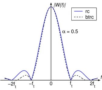
In this way a FFT may still be used instead of the more complex non-power-of-two-DFT and the filter bank orthogonality is restored. The FFT computes the 2N coefficients fk on the windowed samples sw[n]. Fig. 3.5 shows the 2N -FFT filter frequency response (Wrc(f ) and Wbtrc(f )) depending on the roll-off factor.
rc btrc ft 2ft −2ft −ft |W(f)| f α = 0.5 0
Figure 3.5: Raised cosine window and BTRC window depending of roll-off factor α
f
fk fk+1 fk−1
fk−2 fk+2
...
...
Figure 3.6: DFT-filter bank with Nyquist windowing (α = 0)
The filter bank after Nyquist windowing is shown in Fig. 3.6. And as the equation shows yk = 2N −1X n=0 sw[n]e−j2πnk/(2K) = 2N −1X n=0 sw[n]e−j2πn(k/2)/K (3.5)
It is composed of 2N filters separated by ft/2. Equation (3.5) reveals that only the odd or even coefficients contain the carrier information, in this case ...yk−2, yk, yk+2, ....
The other “ghost” coefficients ...yk−3, yk−1, yk+1, ... contain irrelevant information and are not used. We may avoid the computation of these ghost coefficients, decreasing the complexity of the shorted 2N -FFT near to the complexity of the N -FFT (As a example shown below).
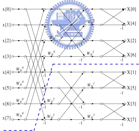
Example:
We assume N = 4, and we need a 2N = 8 FFT in order to implement the Nyquist windowing. A FFT can be graphically represented using butterflies (Fig. 3.7) for 8-point, Wk
N = e−j(2π/N )k)). We can see that one half of the 8-FFT, separated by the dotted line, consists of the odd coefficients and the other half consists of the even coefficients. Therefore it is not necessary to compute one half of the coefficients of the 2N-FFT until the end. We only need to compute the first stage of the 2N -FFT before computing the remaining N-FFT. WN0 WN0 WN0 WN0 WN0 WN0 WN0 WN2 WN2 WN2 WN1 WN3 x[0] x[7] x[6] x[5] x[4] x[3] x[2] x[1] X[0] X[7] X[6] X[4] X[5] X[3] X[2] X[1] -1 -1 -1 -1 -1 -1 -1 -1 -1 -1 -1 -1
3.1.2.1 “Folding” method
If we observe (3.5) further, it can be rewrite as follows : yk = N −1X n=0 sw[n]e−j2πn(k/2)/K + 2N −1X n=N sw[n]e−j2πn(k/2)/K (3.6) = N −1X n=0
(sw[n] + sw[n + N ])e−j2πn(k/2)/K if k ∈ even numbers (3.7)
After multiplying the received sequence in an OFDM symbol by the window function, the last V samples in GI, which are covered by the window function, are added to the last V samples in the symbol. Then, GI is excluded and the remaining N samples are fed into the FFT module. Let k = 2k0 we can rewrite (3.7) as
yk0 =
N −1X n=0
˜
s[n]e−j2πnk0/K , k0 = 0, 1, ..., N − 1 (3.8)
where ˜s[n] = sw[n] + sw[n + N ] for n = 0, 1, ..., N − 1. ˜s[n] is referred to as the “folding window signal”.
In summary, as a shortened 2N -FFT avoids the computation of ghost coefficients, we find that 2N -FFT can be replaced by N -FFT with proper processing before the FFT operation as shown in Fig. 3.8 [20] [21].
Sym bol
GI
t
t
t
0
0
0
G -1
N +G -1
N sam ples
V sam ples
1
0
Nyquist window
G -V
N +G -V
N
N -V
3.1.3
Effect of windowing on ICI and noise Power
3.1.3.1 ICI Analysis
After a width-2N windowing, the received signal part with a normalized CFO fe is
yk = 1 N 2N −1X n=0 s[n]w[n]e−j2πnk/(2N ) = N X m=0 am ( 1 K 2N −1X n=0 w[n]e−j2πn(k/2−m)/Nej2πfen/N ) = N X m=0 am ( 1 K N −1X n=0 (w[n] + w[n + N ])e−j2πn(k/2−m)/Nej2πfen/N ) if k ∈ even numbers = N X m=0 am ( 1 K N −1X n=0 wN[n]e−j2πn(k/2−m)/Nej2πfen/N ) if k ∈ even numbers (3.9) where wN[n] = w[n] + w[n + N ] n = 0, 1, ..., N − 1
After even sampling, i.e. letting k = 2k0, we have
yk0 = ak0W0fe + X m6=k0 amWkf0e−m | {z } ICI for 0 ≤ k0 ≤ N − 1 (3.10) where Wfe
k is the N -FFT of wN(n) with fe. Hence,the power of the desired signal is
σk0 = |ak0|2|W0fe|2 (3.11)
and the corresponding ICI power is σICIk0 = N −1 X m=0,m6=k0 N −1X n=0,n6=k0 ama∗nW fe m−k0W fe n−k0 (3.12)
The ICI power depends not only on the desired symbol location, k0, and the transmitted symbol sequence but also on the pulse-shaping function and the number of subcarriers. Taking average over different independent data sequences on (3.12) gives the average ICI power σk0 ICI = N −1X m=0,m6=k0 |Wfe m−k0| 2 (3.13)
For the Nyquist window pulse, one has (see Fig. 3.5) |Wfe r,m−k0| ≥ |W fe rc,m−k0| (3.14) |Wfe r,m−k0| ≥ |W fe btrc,m−k0| (3.15)
Therefore, a rectangular pulse-shaped OFDM system always has larger ICI power than that associated with a raised-cosine shaped OFDM system or a BTRC pulse-shaped OFDM system. Fig. 3.9 compares the ICI power when α = 0.1 for the rectan-gular pulse, raised-cosine pulse and BTRC pulse. Fig. 3.10 shows a similar comparison for the case of α = 1. Noteworthy, for the same value of α, the BTRC pulse outperforms the raised-cosine pulse despite the fact that the tails of Wbtrc(f ) and Wrc(f ) decay as f−2 and f−3 , respectively. This is because the sum (3.13) is completely dominated by the closest two terms.
Comparing Fig. 3.9 and Fig. 3.10, we find that increasing α leads to large ICI power reduction. This is expected since increasing α corresponds to reducing the side-lobes in the spectrum.
We now examine the impact of the baseband pulse used in terms of the average signal power to average ICI power ratio (SIR). Averaging (3.11) over all possible transmitted symbols and combining with (3.12) yields
SIR = |W fe 0 |2 PN −1 m=0,m6=k0|W fe m−k0|2 (3.16) Fig. 3.11 compares the SIR for different pulse-shaping functions in a 64-subcarrier OFDM system plotted as functions of the normalized frequency offset, fe. Observe that the BTRC pulse outperforms the raised-cosine pulse. For example, assume that it is desired to track CFO range less than 0.25. When employing the BTRC pulse, the SIR can maintain at least 7.1656 dB. In contrast, the SIRmin is only 6.8966 dB when one uses the raised-cosine pulse. The difference of SIRmin between two pulses will become wider as α increases.
0.05 0.1 0.15 0.2 0.25 0.3 0.35 0.4 0.45 0.5 −22 −20 −18 −16 −14 −12 −10 −8 −6 −4 −2
Normalized Frequency Offset fe
Power of ICI(dB)
BTRC pulse (α=0.1) raised cosine pulse (α=0.1) rectangular pulse
Figure 3.9: Comparison of ICI power for different baseband pulse-shaping functions (α = 0.1) in a 64-subcarrier OFDM system.
0.05 0.1 0.15 0.2 0.25 0.3 0.35 0.4 0.45 0.5 −40 −35 −30 −25 −20 −15 −10 −5 0
Normalized Frequency Offset fe
Power of ICI(dB)
BTRC pulse (α=1) raised cosine pulse (α=1) rectangular pulse
Figure 3.10: ICI power associated with different base pulse-shaping functions (α = 1) in a 64-subcarrier OFDM system.
0.05 0.1 0.15 0.2 0.25 0.3 0.35 0.4 0.45 0.5 −5 0 5 10 15 20 25
Normalized Frequency Offset fe
SIR(dB)
BTRC pulse (α=0.1) raised cosine pulse (α=0.1) rectangular pulse
Figure 3.11: SIR for different baseband pulse-shaping functions (α = 0.1) in a 64-subcarrier OFDM system.
3.1.3.2 Noise power analysis
The noise component of the received frequency domain samples at subcarrier k can be written as
nk = 2N −1X
n=0
n0[n]w[n]e−j2πnk/2N (3.17)
where n0[n] is independent complex Gaussian random noise value before windowing at time n and has zero mean and variance σ2
n0 = N0. The power of the noise on sub-carrier
k is σn2 = E[nkn∗k] = 2N −1X m=0 2N −1X n=0 E[ n0[m]n0∗[n] ] w[m]w∗[n] e−j2πnk/2Nej2πnk/2N = σn20 2N −1X m=0 |w[m]|2 (3.18)
Since P2N −1m=0 |w[m]|2 = 1 2N
P2N −1
k=0 |Wk|2 (by Parseval’s Theorem ), one can easily con-clude that with proper Nyquist window, it will not only reduce the ICI power but also the noise power.
3.1.4
Complexity issue
The complexity of an N -FFT may be measured by the number of complex multiplications performed M . The sums (additions) does not represent a major increase in complexity since they may be performed very easy. For a radix-2 algorithm [8],
M = N
2 log2(N ) (3.19)
2N -FFT : As shown in Fig. 3.7. Since the first stage of a FFT normally consists of trivial multiplications (1 ,- 1, j, - j), the complexity of the N -FFT (M multiplications, N sums) is nearly the same that the complexity of the “shorted” 2N -FFT (M non-trivial multiplications, 2N sums).
“Folding” method: After the variable length of CP multiplied by the V samples of window and are added to the last V samples in the symbol, the remaining V samples are fed into the N -point FFT module whose complexity is almost the same as a 2N -point FFT. We thus conclude that the receiver windowing is a computationally reasonable operation.
3.2
Reducing the Number of Trellis States
The complexity of the joint estimation algorithm is mostly associated with the Viterbi search. The state number is M2L states where M is the modulation order and 2L is the considering “CFO channel length” (Section 2.1.2). It will cause time-consuming search if the modulation order is large; The complexity grows exponentially with the number of transmit antennas (M2L∗MT states) if we extend the algorithm to MIOM OFDM systems
(Chapter 4).
the complexity of the Viterbi algorithm by “shortening” the memory of the “CFO chan-nel”.
Since the BTRC window has best property to lower the ICI effect among rectangular window and raised-cosine window, it becomes our favorable candidate.
Consider a residual CFO less than 20% of the subcarrier spacing, we would like to direct truncation of the nonsignificant side channel response. Here, we judge tap Wfe
k to be non-significant if |Wfe k |2/ P k|W fe
k |2 < 0.01. As shown in Fig. 3.12 for BTRC window, there has only three taps after truncation.
Further, we use delayed decision-feedback sequence estimation (DDFSE) algorithm[22], and force the number of considering channel taps down to 2. The algorithm combines structures of the reduced-state Viterbi algorithm and decision-feedback detector and provides a tradeoff between complexity and performance.
−4 −3 −2 −1 0 1 2 3 4 0 0.1 0.2 0.3 0.4 0.5 0.6 0.7 0.8 0.9 1 Subcarriers Power percentage 89.61% 5.47% 0.98% 2.36% 0.61% 0.33% 0.23%
Figure 3.12: Power percentage distribution of BTRC in frequency domain for each sub-carrier at CFO = 0.2.
3.2.1
Complexity issue
Since the total levels of the “reduced-state” approach are the same as the “full-state” approach in Viterbi search, we consider the complexity across two levels only. For the “full-state” approach, one has to compute M branches for every node with 2L+1 complex multiplications performed at each branch. The total number of nodes is equal to M2L. So, M2L× M(2L + 1) = (2L + 1)M2L+1 complex multiplications and M2L comparisons are needed to enter the next level (here L = 2 is used). On the other hand, the “reduced-state” approach used here needs M × M × 3 = 3M2 complex multiplications and M comparisons only.
3.3
Channel Estimation
Since in our CFO estimator for frequency-selective Channels (Section 2.2), the initial channel estimate comes directly from the previous OFDM symbol, the performance of the present symbol is dependent on that of the previous symbol and error propagation is likely to occur. We now examine the effectiveness of the novel model-based estimation method [24] for estimating channels.
3.3.1
Jakes model
The Jakes fading model is a deterministic method for simulating time-correlated Rayleigh fading waveforms [23] and is widely used today. The model assumes that N equal-strength rays arrive at a moving receiver with uniformly distributed arrival angles αn, such that ray n experiences a Doppler shift ωn = ωMcos(αn), where ωM = 2πfcv/c is the maximum Doppler shift, v is the vehicle speed, fc is the carrier frequency, and c is the speed of light. Using αn= 2πn/N (see Fig. 3.13), there is quadrantal symmetry in the magnitude of the Doppler shift, except for angles 0 and π. As a result, the fading waveform can be modelled with N0+ 1 complex oscillators, where N0 = (N/2 − 1)/2.
1
Figure 3.13: Ray arrival angles in the Jakes model (N = 10).
This gives
T (t) = K{√1
2[cos(α) + j sin(α)] cos(ωMt + θ0) +
N0
X n=1
[cos(βn) + j sin(βn)] cos(ωnt + θn)} (3.20)
K is a normalization constant, α (not the same as αn.) and βn are phases, and θn, are initial phases usually set to zero. Setting α = 0 and αn = πn/(N0+ 1) gives zero cross-correlation between the real and imaginary parts of T(t).
Jakes model is a very popular channel model for mobile multipath channels that takes into account the Doppler effect and is based on the assumptions that the receiver is moving at speed v while the arrival angles of multipath components are uniformly distributed. The time correlation of the channel is given by
R(∆t) = J0(2π · ∆t · fd) (3.21)
where Doppler frequency fd = v · fc/c. J0(x) is the zero-th order Bessel function of the first kind.
10 20 30 40 50 60 10 20 30 40 50 60 −0.6 −0.4 −0.2 0 0.2 frequency(Hz) Real part of channel : chv = 108 km/hr
time(sec)
channel response
Figure 3.14: Real part of a Jakes fading process.
3.3.2
Model-based channel estimate
(2.14) of Section 2.2 gives an LS channel estimate which can be rewritten as ˆ Hls(m, n) = R(m, n) X(m, n) = H(m, n) + N oise(m, n) + ICI(m, n) X(m, n) , (3.22)
where H(m, n), X(m, n) and R(m, n) denote respectively the channel response, trans-mitted signal and received samples at the mth subcarrier during the nth symbol interval. The channel responses H(m, n) can be viewed as a sampled version of the two-dimension (2D) continuous complex fading process H(f, t) (Fig. 3.14). We choose a operating region in the time-frequency plane and model the sampled fading process H(m, n) in this region by the quadrature surface
where the coefficients (a, b, c, d, e, f ) are chosen such that X (m,n) ¯ ¯ ¯ ˆHls(m, n) − Hmodel(m, n) ¯ ¯ ¯2 (3.24)
is minimized. Rewriting (3.24) in a more compact form X (m,n) ¯ ¯ ¯ ˆHls(m, n) − qTm,nc ¯ ¯ ¯2 (3.25)
where cH = (a, b, c, d, e, f ) is the coefficient vector and qT
m,n = (m2, mn, n2, m, n, 1) is the data location vector, we can show
ˆc = arg min c ¯ ¯ ¯ ¯ ¯ ¯ ˆHls− Qc ¯ ¯ ¯ ¯ ¯ ¯ 2 (3.26) where ˆHls= ( ˆHls(0, 0), ˆHls(0, 1), ..., ˆHls(Lf − 1, Lt− 1))T and Q = qT 0,0 qT 0,1 ... qT Lf−1,Lt−1 = 0 0 0 · · · 1 0 0 1 · · · 1 ... ... ... . .. ... (Lf − 1)2 (Lf − 1)(Lt− 1) (Lt− 1)2 · · · 1 Lf and Lt are the block length of freq and time respectively. Note that from (3.23) Qˆc represents the new estimate of the channel impulse response. By solving (3.26), the coefficients of the regression polynomial is
ˆc = (QTQ)−1QTHˆ
ls, (3.27)
and we obtain the new estimates ˆ Hmodel(m, n) = qTm,nˆc. (3.28) ˆ Hmodel = Qˆc = Q(QTQ)−1QTHˆls= V ˆHls, (3.29) where V = Q(QTQ)−1QT. (3.30)
Fig. 3.15 indicates the fitting processing of one-dimension (1-D). We can infer that if the SNR is high enough, the regression may improve the channel estimation.
real channel LS 1−D regression
Figure 3.15: Regression of LS channel under SNR=12dB.
3.3.3
2D model-based channel estimate with transform-domain
processing (2-D+TDP)
A channel estimation based on transform-domain processing was proposed in [25]. This method employs lowpass filtering in the transform domain so that ICI and additive AWGN components in the received pilots are significantly reduced.
Although we can not get the information from a side band, we can still use the regression model of the previous subsection to suppress the effects of ICI and AWGN in the transform-domain. Fig. 3.16 is a block diagram that represents an improved channel estimator, concatenating the transform-domain processing algorithm with the 2D model-based channel estimator.
Least-Square
channel estimation Transform-domainprocessing Model-based channelestimation
H
LSH
TDH
modelr
3.3.4
Complexity issue
Suppose there are Numodulated subcarriers in the transmitted waveform, an LS channel estimate needs Nucomplex divisions or 5Npmultiplications per OFDM symbol. It is thus preferred to use (3.29) from a complexity point of view. The resulting computational algorithm is
ˆc = P ˆHls, (3.31)
ˆ
Hmodel(m, n) = qTm,nˆc. (3.32)
where P = (QTQ)−1QT
is a constant matrix with dimension length(c) × (Lf · Lt). To obtain ˆc we need 2 length(c)LfLt real multiplications since P is real. Calculating each channel response at the data tone using (3.32) needs 2 LfLt real multiplications. Since there are Nu modulated subcarriers, we totally need 2Nu(length(c) + 1)LfLt real multiplications for an OFDM symbol.
The transform-domain based channel estimate uses two FFTs (both of size is Nu) to estimate the channel response. For a radix-2 algorithm, the total number complex multiplications required is about Nulog2(Nu) and need 2Nu(length(c) + 1)Lf real mul-tiplications for regression in the transform-domain. On the other hand, the proposed 2-D regression model needs LfNu memory to store those symbols information. The 1D channel estimate does not need any extra memory to save symbol information.
3.4
Numerical Experiments
In previous sections, we have presented several methods either to enhance perfor-mance or to reduce complexity of a joint estimation-detection process. This section gives some numerical experimental results on these improvements. We first compare the BER performance of the conventional Nyquist window (raised-cosine window) with that of rectangular windowing in AWGN channels (Fig. 3.17). In Fig. 3.18, we then pro-ceed to examine the performance in Rayleigh fading channels. We find that the BTRC
window offers a superior performance for OFDM systems with nonzero CFO. One ob-serves that the BER performance is almost undistinguishable for different windowing at small SNRs. This is because BER performance is dominated by AWGN at small SNRs and is determined by the ICI at high SNRs. The almost-flat curve represents the per-formance of a receiver that does not update channel estimate, using the pilot-assisted estimate for detecting the data payload. It obvious that channel updates are needed in a time-varying channel to have reliable decisions. Fig. 3.19 proves the importance of the channel estimation method used and indicates that the regression model-based algorithm does offer reliable channel estimates. Finally, Fig. 3.20 reveals that the reduced-state algorithm is effective for it incurs less than 0.6 dB BER performance loss within the range of interest.
0 1 2 3 4 5 6 7 8 9 10 10−6 10−5 10−4 10−3 10−2 10−1 100 SNR (dB) BER fe=0.1:rectangular fe=0.1:raised−cosine (α=0.1) fe=0.2:rectangular fe=0.2:raised−cosine (α=0.1) fe=0.4:rectangular fe=0.4:raised−cosine (α=0.1)
Figure 3.17: BER performance of SISO-OFDM systems using iterative joint FD estimate with different windowing in AWGN channels.
10 12 14 16 18 20 22 10−3 10−2 10−1 100 SNR (dB) BER fe=0.2:rectangular fe=0.2:raised−cosine (α=0.1) fe=0.2:BTRC (α=0.1) Perfect Channel of BTRC Without Update Channel of BTRC
Figure 3.18: BER performance of SISO-OFDM systems using iterative joint FDC esti-mate with different windowing in Rayleigh fading channels.
10 12 14 16 18 20 22 10−3 10−2 10−1 100 SNR (dB) BER fe=0.2:BTRC (α=0.1) fe=0.2:BTRC 1−D (α=0.1) fe=0.2:BTRC 1−D+TDP (α=0.1) fe=0.2:BTRC 2−D+TDP (α=0.1) Perfect Channel of BTRC
Figure 3.19: Effect of channel estimate on the SISO-OFDM system’s BER performance.
10 12 14 16 18 20 22 10−2 10−1 100 SNR (dB) BER fe=0.2:BTRC (α=0.1)
fe=0.2:BTRC reduced state algorithm (α=0.1)
Figure 3.20: BER performance of SISO-OFDM systems using iterative joint FDC esti-mate with reduced-state DF method in Rayleigh fading channels.
Chapter 4
Joint Estimation for MIMO-OFDM
Systems
4.1
Introduction
The efficiency of a communication system is often judged by how the main resources– power and signal dimensionality–is used. Until recently, the latter is measured by the time-bandwidth product of the transmitted waveform. By exploiting the degrees of freedom of the spatial domain, one is able to significantly increase the capacity of a wireless system [26] [27]. The spatial degrees of freedom is realized by using multiple antennas at both transmitter and receiver, generally referred to as the multiple-input multiple-output (MIMO) technologies.
The high spectral efficiency associated with a MIMO channel is achieved under the assumption that a richly scattering environment renders independent propagation paths between each pair of transmit and receive antennas. In a MIMO system, high-rate data transmission is accomplished by de-multiplexing, i.e., dividing the original data stream into several parallel data substreams, each of which is transmitted from a corresponding transmit antenna. All data substreams are independent of each other and different data substreams will result in co-antenna interference (CAI) upon reception. A well-known realization is the BLAST (Bell Labs Layered Space Time) system [28] that achieves high peak throughput with small constellations.
The OFDM scheme has been adopted by the wireless local-area-network (WLAN) standards IEEE 802.11a and 802.11g due to its high spectral efficiency and ability to combat frequency selective fading and narrowband interference. Thus if CAI can be mitigated, a MIMO-OFDM system can provide both high data rates and improved system performance through the use of the antenna as well as the frequency diversities. Since the throughput enhancement of MIMO is especially high in richly-scattered scenarios of which indoor environments are typical examples, the widespread indoor deployments of WLAN systems makes MIMO-OFDM a strong and natural candidate for high throughput extension (802.11n) of the current WLAN standards.
This chapter examines the most critical design issue associated with a MIMO-OFDM system, namely, the problem of frequency compensation, channel estimation and data detection. We will explain why it is possible and indeed feasible to extend the joint FDC estimation algorithm we presented in the last chapter to a MIMO-OFDM environment.
4.2
System Model
Consider a MIMO system with MT transmit antennas and MR receive antennas. As-suming a flat block-fading channel model, we can express the equivalent signal part of the received time-domain samples at qth receive antenna as
bq[n] = MT X p=1 ˜ sq,p[n], q = 1, 2, . . . , MR. (4.1) where ˜ sq,p[n] = 1 N N −1X k=0 r Es MT apkHkq,pej2πnk/Nej2πfen/N (4.2)
corresponds to the OFDM signal sent from the pth transmit antenna to the qth receive antenna. Moreover,
• Hkq,p is the kth subcarrier’s channel transfer function between the qth receive an-tenna and the pth transmit anan-tenna,
• Es is the average energy allocated to the kth subcarrier across the transmit anten-nas,
• fe is the CFO normalized by the inter-carrier spacing, and
• N is the total number of sub-carriers for each transmit antenna.
After establishing proper frame (symbol) timing, removing the cyclic prefix and taking FFT on the time-domain samples, the received baseband frequency domain signal at the qth RX antenna reads rqk = N −1X n=0 ˜bq[n]e−j2πnk/N + nq k = MT X p=1 N −1 X m=0 apmHmq,pWfe k−m+ n q k = MT X p=1 yk(fe, ap, Hq,p) + nqk, q = 1, 2, . . . , MR. (4.3)
where ˜bq[n] is the “folding window signal” from all transmit antennas.
Fig. 4.1 plots the transmission channel model for the qth receive antenna with respect to MT transmit antennas. Comparing the above equation with (2.13), we find that to apply the joint FDC method to solve (4.3), we will have a trellis with the number of trellis states equals to M2L∗MT since we now have to consider all transmitted data
streams from all transmit antennas.
4.3
MIMO-OFDM Channel Estimation
Rewriting (4.3) in matrix form (for qth RX antenna) rq0 rq1 ... rN −1q = Wfe 0 · · · W fe −N +1 ... . .. ... Wfe N −1 · · · W fe 0 PMT p=1H q,p 0 a p 0 PMT p=1H q,p 1 a p 1 ... PMT p=1H q,p N −1a p N −1 + nq0 nq1 ... nqN −1 (4.4)
C hannel between T Xp and RXq C hannel between T X1 and RXq C hannel between T XM T and RXq T X1 T Xp T XM T A WG N at RXq R Xq C FO between T X and RX
Figure 4.1: Channel model for the qth receive antenna.
and invoking the substitutions,
rq = [r0q r1q · · · rN −1q ]T (4.5) n = [nq0 nq1 · · · nqN −1]T (4.6) HqA = [(HqA)0 (HAq)1 · · · (HqA)N −1]T (4.7) = "MT X p=1 H0q,pap0 MT X p=1 H1q,pap1 · · · MT X p=1 HN −1q,p apN −1 #T (4.8) F = Wfe 0 · · · W fe −N +1 ... . .. ... Wfe N −1 · · · W fe 0 (4.9) we obtain rq = FHqA+ n. (4.10)
Assuming the data sequence and the CFO are known, we first compensate for the CFO through the LS estimate
b HqA = h( bHqA)1 ( bH q A)2 · · · ( bH q A)N −1 iT = (FHF)−1FHrq (4.11)
The kth subcarrier over MR receive antennas reads
( bHA)k,t = h ( bH1A)k,t ( bH 2 A)k,t · · · ( bH MR A )k,t iT (4.12) Ak,t = [a1k,t a2k,t · · · a MT k,t ]T (4.13)
where the index 1 ≤ t ≤ M denotes the tth OFDM symbol of an M-symbol block that suffer from the same flat (block-)fading.
Stacking up the M received frequency domain symbols we have
( bHA)k = bHkAk (4.14)
where
( bHA)k = [( bHA)k,1 ( bHA)k,2 · · · ( bHA)k,M]
Ak = [Ak,1, Ak,2, · · · , Ak,M] (4.15)
and bHk is the MR× MT complex channel matrix for the kth subcarrier. Finally, the channel matrix can be estimated by
b Hk= ( bHA)k A H k (AkA H k)−1 (4.16)
on the premise that the rank of Ak, the “over symbols data matrix at subcarrier k” is greater than MT. In other words, one has to sent at least MT OFDM symbols over the same flat fading block (a coherent time) in order to obtain a proper channel estimate [29].
4.4
An Iterative Joint FDC Estimation Algorithm
Based on the above discussion, we suggest an iterative joint FDC estimation algorithm as follows.
C.1 (Channel estimate initialization) Set bHO to be the channel estimate from the previous OFDM symbols.
C.2 (Frequency Estimate Initialization) Set the initial estimate ˆfe = 0.
C.3 (Starting the FD iteration loop) Use current channel estimate for the frequency-data sequence iteration loop. Calculate the channel frequency response compen-sation matrix F = [Wfe
k ] based on (4.9) and current frequency estimate ˆfe.
C.4 (Compute the tentative data estimate) Given the observed sample vector r defined by (4.5), perform the Viterbi algorithm with the branch metric
λqk= ¯ ¯ ¯ ¯ ¯r q k− M T X p=1 yk( ˆfe, ap, bH q,p ) ¯ ¯ ¯ ¯ ¯ 2 (4.17) to find a conditional optimal data sequence estimate ˆa
C.5 (Update the frequency estimate) Update the CFO estimate by minimizing the cost function : C = X q X k ¯ ¯ ¯ ¯ ¯r q k− M T X p=1 yk(fe, ˆap, Hq,p) ¯ ¯ ¯ ¯ ¯ 2 (4.18)
C.6 (Convergence check and end of the FD loop) If the new CFO estimate ˆfe is close to the previous estimate, i.e. absolute difference is less than 10−6, then stop the current FD iteration and release the new estimates ˆa and ˆfe; otherwise go back to Step 3.
C.7 (Channel estimate update) Compute a new channel estimate bHN using (4.16) based on the current estimates ˆfe and ˆa.
C.8 (Convergence check for the channel estimate) If the new channel estimate bHN is close enough to the previous estimate, more specifically, if
¯ ¯ ¯ ¯ ¯ ˆ HN − ˆHO ˆ HN ¯ ¯ ¯ ¯ ¯ 2 < 10−2
then stop iteration and release the most recent estimates. Otherwise, go to Step 3.
4.5
Numerical Experiments
The simulation parameters and environments used in the following paragraphs are identical to those used in the SISO-OFDM system simulations, except that we now have MT × MR independent channels. The BER performance of the iterative joint FDC es-timation algorithm for the 2 × 2 configuration is given in Fig. 4.2. For comparison purpose the SISO performance curve is shown in the same figure. Clearly, the spatial diversity does pay off–with a gain of more than 4 dB for BER < 10−2. The MSEE per-formance of the corresponding frequency estimate is plotted in Fig. 4.3. Similarly, we find that more receive antennas leads to better performance due to the MIMO diversity gain. Fig. 4.4 shows the effect of the channel estimate on the BER performance. These curves indicate that, as expected, the model-based channel estimation still outperform the LS channel estimate for MIMO-OFDM systems.
10 12 14 16 18 20 22 10−3 10−2 10−1 SNR (dB) BER 1 TX 1 RX 2 TX 2 RX
Figure 4.2: BER performance of MIMO- and SISO-OFDM systems using iterative joint FDC estimate (fe = 0.2). 10 12 14 16 18 20 22 −37 −36 −35 −34 −33 −32 −31 SNR (dB)
MS CFO Estimation Error (dB)
1 TX 1 RX 2 TX 2 RX
Figure 4.3: MSEE performance of CFO estimates in MIMO-OFDM systems for 2 × 2 and SISO configurations (fe = 0.2).
10 12 14 16 18 20 22 10−4 10−3 10−2 10−1 SNR (dB) BER 2 TX 2 RX 2 TX 2 RX 1−D+TDP 2 TX 2 RX 2−D+TDP 2 TX 2 RX known channel
Figure 4.4: Effect of the channel estimate on the MIMO-OFDM system’s BER perfor-mance (fe = 0.2).
Chapter 5
Conclusion
We have presented iterative joint estimation and detection algorithms for OFDM systems in various scenarios. An iterative joint frequency estimation and data sequence detection algorithm is first given for AWGN channels. By incorporating a proper chan-nel estimation method, we then provide an iterative joint FDC estimation algorithm for SISO-OFDM systems. Some refinements for enhanced performance and complexity reduction are suggested. Finally, we extend the our joint FDC estimation algorithm to MIMO-OFDM environments. Simulation based on a candidate IEEE 802.11n standard– the Tgn Sync (Task Group n) proposal–is provided to validate various joint estimation and detection algorithms. The corresponding numerical results do prove that the pro-posed solutions are both practical under the assumed channel conditions. Our solution can operate in the blind mode if the initial CFO is less than half of a subcarrier spacing. Otherwise, we can use the preamble (like the 802.11n case) to reduce the CFO to within the desired range. Our proposal can then be used for subsequent data detection and CFO/channel tracking in time-varying channels.