Geometric analysis on generalized
Hermite operators
Der-Chen Chang∗ and Sheng-Ya Feng†
February 2, 2010
Abstract: In this paper, we shall by using Hamiltonian and Lagrangian formal-ism to study the generalized Hermite operator: L = −Pnj=1 ∂2
∂x2 j +
Pn
j,k=1bjkxjxk.
Given two points x0 and x in Rn, we count the number of “geodesics”
connect-ing these two points. Here geodesics are defined as the projection of solutions of the Hamiltonian system onto the x-space. Then we construct the action function. Using the famous Van Vleck’s formula, one may construct the heat kernel for the operator ∂t∂ − L.
Key words: Hermite operator, Hamiltonian function, Lagrangian, Euler-Lagrange equation, heat kernel
MS Classification (2000): Primary: 35J05; Secondary: 35F21
1
Introduction
In this paper, we shall by using Hamiltonian and Lagrangian formalism to study the heat kernel for the following operator
L = − n X j=1 ∂2 ∂x2 j + n X j,k=1 bjkxjxk. (1.1)
When bjk = δjk, the operator L = −
Pn
j=1 ∂
2
∂x2
j+|x|
2is the Hermite operator
which arise from harmonic oscillator. This operator arises in many contexts and has been studied by mathematicians and physicists for quite some time
(see e.g., [1], [2], [7], [8]). When bjk = −δjk, the operator L reduces to
−Pnj=1 ∂2
∂x2
j − |x|
2 which arise from anti-harmonic oscillator (see e.g., [11]).
This is the reason we call the operator L generalized Hermite operator. A common method to deal with the Hermite operator by using Hermite functions {ψk(x)}∞
k=0 which are defined by their generating function ∞ X k=0 ψk(x) k! t k= e2tx−t2−x2 2 .
The function ψk(x) is the eigenfunction of x2− d
2
dx2 with eigenvalue 2k + 1
([10]). One may use the Fourier transform method to obtain the heat kernel as follows: K(x0, x; t) = 1 (2π)n2 v u u tYn k=1 1 sinh(t)e −1 2(kx0k2+kxk2) coth(t)+sinh(t)x0·x = 1 (2π)n2 v u u tYn k=1 1 sinh(t)e −1 2 Pn k=1[(xk+x0k)2tanh(t2)+(xk−x0k)2coth(t2)]. (1.2) For more detailed discussion, readers may see e.g., [4], [6]. However, there are no eigenfunctions for the operator L with a general quadratic form B. In this paper, we are going to use geometric mechanics to study the heat kernel for the operator L. The Hamiltonian function for L is
H(x, ξ) = − n X j=1 ξj2+ n X j,k=1 bjkxjxk= −ξtξ + xtBx where ξ = [ξ1, . . . , ξn]t and x = [x1, . . . , xn]t and B = [bjk] ∈ Mn×n(R).
It follows that the Hamilton system is ( ˙x = +∂H∂ξ = −2ξ ˙ξ = −∂H ∂x = −(B + Bt)x (1.3) Since h ˙x, ~eji = −2hξ, ~eji
and h ˙ξ, ~eji = − ³ hBx, ~eji + h~ej, Btxi ´ = −h(B + Bt)x, ~eji, one has ¨ x = −2 ˙ξ = 2(B + Bt)x := Ax (1.4) where A = 2(B + Bt) = · a b b d ¸ .
In order to solve the system (1.4), denote y = ˙x. Then · ˙x ˙y ¸ = · 0 In A 0 ¸ · x y ¸ (1.5) where In is the n × n identity matrix.
Using the results for ordinary differential equations, we can solve the system (1.5). Let us first observe that the eigenvalues of the matrix
· 0 In A 0 ¸ are det µ λI2n×2n− · 0 In A 0 ¸¶ = det · λIn −In −A λIn ¸ = det(λ2In− A) = 0
In other words, λ2 are the eigenvalues of A. Since A is symmetric, hence A has n real eigenvalues µj, j = 1, . . . , n. This implies that the fundamental
solution for the system (1.5) is the linear combination of the following:
Pj(s)e± √µ
js when µ j ≥ 0,
where Pj(s) is a polynomial whose degree does not exceed the multiplicity
of µj and
Pk(s) cos¡√−µks¢ and Pk(s) sin¡√−µks¢
when µk< 0. Here Pk(s) is a polynomial whose degree does not exceed the multiplicity of µk. Therefore, we just gave a detailed discussion when n = 2.
The method can be generalized to a high dimension case easily.
Given two distinct points x0, xτ in Rn, we call the projection of solutions
of the system (1.3) (with boundary conditions x(0) = x0 and x(τ ) = xτ) onto the x-space a “geodesic” connecting these two points (see e.g., [3]). As we expect, there is only one solution for this system when the matrix
geodesics connecting these two points. But, there exists some situations for which no geodesic connecting x0 and xτ. We shall give a detailed discussion
in cases (5) to (8). Then we will construct action function for the operator
L by using Lagrangian formalism. In order to construct heat kernels, one
also needs to construct “volume elements”. Since the potential is quadratic, we can use the famous Van Vleck’s formula to achieve this goal (see e.g., see [9] and [6]). In the last section, we shall show that these kernel functions satisfy generalized heat kernel properties.
A significant part of this research project was completed when the second author visits Georgetown University supported by the China Scholarship Council during the 2009-2010 academic year. He takes great pleasure in expressing his thanks to the Department of Mathematics at Georgetown University for the invitation and the warm hospitality during his visit in United States.
The final version of this paper is based on the talk given by the first au-thor during the 2009 Taiwan-Norway Workshop on Geometric Analysis and Mathematical Physics, which was held on December 14-16 at the National Center for Theoretical Sciences in Hsinchu, Taiwan. The first author takes great pleasure in expressing his thanks to Professor Winnie Li, the director of NCTS, for the invitation and the warm hospitality during his visit in Taiwan.
2
Solving the Hamiltonian system when n = 2
For n = 2 the operator (1.1) becomes
L = −³ ∂ 2 ∂x2 1 + ∂ 2 ∂x2 2 ´ + b11x21+ (b12+ b21)x1x2+ b22x22.
The associated Hamiltonian function is
H = −(ξ12+ ξ22) + b11x21+ (b12+ b21)x1x2+ b22x22.
Hence, the Hamiltonian system is (
˙x = ∂H∂ξ ˙ξ = −∂H
This implies that ˙x1 = ∂H∂ξ1 = −2ξ1 ˙x2 = −∂H∂ξ2 = −2ξ2 ˙ξ1 = −∂x∂H1 = − ¡ 2b11x1+ (b12+ b21)x2 ¢ ˙ξ2 = −∂x∂H2 = − ¡ 2b22x2+ (b12+ b21)x1 ¢ (2.6)
where x = [x1, x2]t and ξ = [ξ1, ξ2]t. Hence,
¨ x = Ax where A = 2(B + Bt) = 2 µ 2b11 b12+ b21 b12+ b21 2b22 ¶ = µ a b b d ¶ . Let y1 = ˙x1, y2 = ˙x2, then ˙x1 ˙x2 ˙y1 ˙y2 = µ 0 I2 A 0 ¶ x1 x2 y1 y2 . The characteristic equation is
det µ λI4− µ 0 I2 A 0 ¶¶ = 0 which is equivalent λ4− (a + d)λ2+ (ad − bc) = 0. (2.7) Therefore
D = (a + d)2− 4(ad − b2) = (trA)2− 4 det A = (a − d)2+ 4b2 ≥ 0.
Assume that the eigenvalues of A are µ1 and µ2. Without loss of generality,
we may assume that µ1 ≥ µ2. We are going to discuss the equation (2.7) in
8 cases.
We need to solve the Hamilton’s system (2.6) with boundary conditions: x0 1 = x1(s0) x1 = x1(s1) x02 = x2(s0) x = x (s ) (2.8)
2.1 Case (1). µ1 > µ2 > 0.
In this case, one has a + d >√D > 0. It follows that µ1 = a + d + √ D 2 > µ2 = a + d −√D 2 > 0. Hence, equation (2.7) has four fundamental solutions:
e±√µ1s and e±√µ2s. Let · x1(s) x2(s) ¸ = · c1 c2 c3 c4 c5 c6 c7 c8 ¸ e−√µ1s e√µ1s e−√µ2s e√µ2s . This implies that
· ¨ x1(s) ¨ x2(s) ¸ = · c1 c2 c3 c4 c5 c6 c7 c8 ¸ µ1 0 0 0 0 µ1 0 0 0 0 µ2 0 0 0 0 µ2 e−√µ1s e√µ1s e−√µ2s e√µ2s .
Since ¨x = Ax, then
· c1 c2 c3 c4 c5 c6 c7 c8 ¸ µ1 0 0 0 0 µ1 0 0 0 0 µ2 0 0 0 0 µ2 = · a b b d ¸ · c1 c2 c3 c4 c5 c6 c7 c8 ¸ which is equivalent to · µ1c1 µ1c2 µ2c3 µ2c4 µ1c5 µ1c6 µ2c7 µ2c8 ¸ = · ac1+ bc5 ac2+ bc8 ac3+ bc7 ac4+ bc8 bc1+ dc5 bc2+ dc6 bc3+ dc7 bc4+ dc8 ¸
Assume that b 6= 0, then the above identity is equivalent to c5 c6 c7 c8 = µ1−a b µ 1−a b µ2−a b µ2−a b c1 c2 c3 c4 (2.9)
Plugging in the boundary conditions (2.8), one has 1 1 1 1 e−√µ1τ e√µ1τ e−√µ2τ e√µ2τ µ1−a
b µ1b−a µ2b−a µ2b−a
µ2−a b e− √µ 1τ µ2−a b e √µ 1τ µ2−a b e− √µ 2τ µ2−a b e √µ 2τ x0 1 x1 x02 x2 (2.10) Denote M1= · 1 1 e−√µ1τ e√µ1τ ¸ , M2= · 1 1 e−√µ2τ e√µ2τ ¸ and α1= · x0 1 x1 ¸ and α2 = · x0 2 x2 ¸
We may rewrite the system (2.10) as follows: M1 M2 ... α1 µ1−a b M1 µ2b−aM2 ... α2 → M1 M2 ... α1 0 µ2−µ1 b M2 ... a−µb 1α1+ α2 → M1 0 ... β1 0 M2 ... β2 (2.11) where β1=µa − µ2 1− µ2α1+ b µ1− µ2α2 = · b1 b2 ¸ , β2=µµ1− a 1− µ2 α1−µ b 1− µ2 α2 = · b1 b2 ¸ , and b1 = µa−µ1−µ22x01+ µ1−µb 2x 0 2 b2 = µa−µ1−µ22x1+ µ1−µb 2x2 b3 = µµ11−µ−a2x01− µ1−µb 2x 0 2 b4 = µµ11−µ−a2x1− µ1−µb 2x2 Since for τ > 0, det M1 = e √µ 1τ − e−√µ1τ = 2 sinh¡√µ 1τ ¢ 6= 0,
By (2.11), we know that · c1 c2 ¸ =M1−1β1 = · 1 1 e−√µ1τ e√µ1τ ¸−1"a−µ2 µ1−µ2x 0 1+µ1−µb 2x 0 2 a−µ2 µ1−µ2x1+ b µ1−µ2x2 # , · c3 c4 ¸ =M2−1β2 = · 1 1 e−√µ2τ e√µ2τ ¸−1"µ1−a µ1−µ2x 0 1−µ1−µb 2x 0 2 µ1−a µ1−µ2x1− b µ1−µ2x2 # .
From (2.9), we know that · c5 c6 ¸ =µ1− a b · c1 c2 ¸ = · 1 1 e−√µ1τ e√µ1τ ¸−1" b µ1−µ2x 0 1+ µµ11−µ−a2x 0 2 b µ1−µ2x1+ µ1−a µ1−µ2x2 # , · c7 c8 ¸ =µ2− a b · c3 c4 ¸ = · 1 1 e−√µ2τ e√µ2τ ¸−1" −b µ1−µ2x 0 1+ µa−µ1−µ22x 0 2 −b µ1−µ2x1+ a−µ2 µ1−µ2x2 # .
When b = 0, the discussion is similar. (In fact, the situation is even better since we are dealing a diagonal matrix.) Hence, we just concentrate on the situation when b 6= 0.
2.2 Case (2). µ1 = µ2 > 0.
From the discriminant of the characteristic equation of A, one has a = d =
µ1= µ2 and b = 0 in this case. Hence,
· x1(s) x2(s) ¸ = · c1 c2 c3 c4 c5 c6 c7 c8 ¸ e−√µ1s e√µ1s se−√µ1s se√µ1s . It follows that · ˙x1(s) ˙x2(s) ¸ = · c1 c2 c3 c4 c5 c6 c7 c8 ¸ −√µ1 0 0 0 0 √µ1 0 0 1 0 −√µ1 0 0 1 0 √µ1 e−√µ1s e√µ1s se−√µ1s se√µ1s . Therefore, · ¨ x1(s) ¨ x2(s) ¸ = · c1 c2 c3 c4 c5 c6 c7 c8 ¸ −√µ1 0 0 0 0 √µ1 0 0 1 0 −√µ1 0 0 1 0 √µ1 2 e−√µ1s e√µ1s se−√µ1s se√µ1s .
Since ¨x = Ax, then · c1 c2 c3 c4 c5 c6 c7 c8 ¸ −√µ1 0 0 0 0 √µ1 0 0 1 0 −√µ1 0 0 1 0 √µ1 2 = · µ1 0 0 µ1 ¸ · c1 c2 c3 c4 c5 c6 c7 c8 ¸ which is equivalent to · µ1c1− 2√µ1c3 µ1c2+ 2√µ1c4 µ1c3 µ1c4 µ1c1− 2√µ1c7 µ1c2+ 2√µ1c8 µ1c7 µ1c8 ¸ = · µ1c1 µ1c2 µ1c3 µ1c4 µ1c5 µ1c6 µ1c7 µ1c8 ¸ . This tells us c3= c4= c7= c8= 0.
Plugging in the boundary conditions (2.8), one has 1 1 0 0 e−√µ1τ e√µ1τ 0 0 0 0 1 1 0 0 e−√µ1τ e√µ1τ c1 c2 c5 c6 = x01 x1 x0 2 x2 .
This implies that · c1 c2 ¸ = · 1 1 e−√µ1τ e√µ1τ ¸−1· x01 x1 ¸ , · c5 c6 ¸ = · 1 1 e−√µ1τ e√µ1τ ¸−1· x02 x2 ¸ . 2.3 Case (3). µ1 > µ2 = 0. In this case, · x1(s) x2(s) ¸ = · c1 c2 c3 c4 c5 c6 c7 c8 ¸ e−√µ1s e√µ1s 1 s . It follows that · ¸ · ¸ µ1e −√µ1s √µ s
Since ¨x = Ax, then · c1 c2 c3 c4 c5 c6 c7 c8 ¸ µ1 0 0 0 0 µ1 0 0 0 0 0 0 0 0 0 0 = · a b b d ¸ · c1 c2 c3 c4 c5 c6 c7 c8 ¸
which is equivalent to (if b 6= 0) c5 c6 c7 c8 = µ1−a b µ 1−a b −a b −a b c1 c2 c3 c4 .
Similar to Case (1), the boundary conditions (2.8) gives us a system like (2.11) as follows: 1 1 0 0 ... b1 e−√µ1τ e√µ1τ 0 0 ... b 2 0 0 1 0 ... b3 0 0 1 τ ... b4 where b1= µa1x01+µb1x 0 2 b2= µa1x1+µb1x2 b3= µ1µ−a1 x01−µb1x 0 2 b4= µ1µ−a1 x1−µb1x2
This implies that · c1 c2 ¸ = · 1 1 e−√µ1τ e√µ1τ ¸−1· b1 b2 ¸ , · c3 c4 ¸ = · 1 0 1 τ ¸−1· b3 b4 ¸ = 1 τ · τ 0 −1 1 ¸ · b3 b4 ¸ . 2.4 Case (4). µ1 = µ2 = 0. In this case, · x1(s) x2(s) ¸ = · c1 c2 c3 c4 c5 c6 c7 c8 ¸ 1 s s2 s3 .
It follows that · ¨ x1(s) ¨ x2(s) ¸ = · c1 c2 c3 c4 c5 c6 c7 c8 ¸ 0 0 2 6s . Since ¨x = Ax, then
· c1 c2 c3 c4 c5 c6 c7 c8 ¸ 0 0 0 0 0 0 0 0 2 0 0 0 0 6 0 0 1 s s2 s3 = · 0 0 0 0 ¸ · c1 c2 c3 c4 c5 c6 c7 c8 ¸
This is equivalent to c3 = c4 = c7 = c8 = 0. Using the boundary
condi-tions (2.8), one has 1 0 0 0 1 τ 0 0 0 0 1 0 0 0 1 τ c1 c2 c5 c6 = x0 1 x1 x0 2 x2 . This implies that
· c1 c2 ¸ = · 1 0 1 τ ¸−1· x0 1 x1 ¸ = 1 τ · τ 0 −1 1 ¸ · x0 1 x1 ¸ , · c5 c6 ¸ = · 1 0 1 τ ¸−1· x0 2 x2 ¸ = 1 τ · τ 0 −1 1 ¸ · x0 2 x2 ¸ . 2.5 Case (5). 0 > µ1 > µ2. In this case, · x1(s) x2(s) ¸ = · c1 c2 c3 c4 c5 c6 c7 c8 ¸ cos(√−µ1s) sin(√−µ1s) cos(√−µ2s) sin(√−µ2s) . (2.12) It follows that · ¸ · ¸ µ1cos( √ −µ1s) √
Since ¨x = Ax, then · c1 c2 c3 c4 c5 c6 c7 c8 ¸ µ1 0 0 0 0 µ1 0 0 0 0 µ2 0 0 0 0 µ2 = · a b b d ¸ · c1 c2 c3 c4 c5 c6 c7 c8 ¸
which is equivalent to (if b 6= 0) c5 c6 c7 c8 = µ1−a b µ1−a b µ2−a b µ2−a b c1 c2 c3 c4 . (2.13) Using the boundary conditions (2.8) gives us a system like (2.11) as follows:
Mf1 0 ... β1 0 Mf2 ... β2 . Here f M1= · 1 0 cos(√−µ1τ ) sin( √ −µ1τ ) ¸ , Mf2 = · 1 0 cos(√−µ2τ ) sin( √ −µ2τ ) ¸ and β1 = · b1 b2 ¸ , β2 = · b3 b4 ¸ with b1 = µa−µ1−µ22x01+ µ1−µb 2x 0 2 b2 = µa−µ1−µ22x1+ µ1−µb 2x2 b3 = µµ11−µ−a2x01− µ1−µb 2x 0 2 b4 = µµ11−µ−a2x1− µ1−µb 2x2
First, we need to know that for j = 1, 2, det fMj = 0 ⇔ sin( p −µjτ ) = 0 ⇔p−µjτ = kjπ, kj ∈ N. In other words, 2 X j=1 ¡ det fMj ¢2 = 0 ⇔ (√ −µ1τ = k1π √ −µ2τ = k2π ⇔ √ −µ1 √ −µ2 = k1 k2.
2.5.1 √√−µ1
−µ2 ∈ Q.
In this case, det fM1and det fM2vanish or nonvanish simultaneously. Suppose that √√−µ1 −µ2 = K1 K2 with (K1, K2) = 1. Then (A). τ = √K1 −µ1mπ, m ∈ N. In this case, P2 j=1 ¡
det fMj¢2 = 0. There are two cases here.
(A.1). b2 = (−1)K1mb1 and b4 = (−1)K2mb3, then system (2.13) for cj,
j = 1, 2, 3, 4 has infinite number of solutions.
Now we discuss the solutions of the system (
b2 = (−1)K1mb1
b4 = (−1)K2mb3
(2.14) When b = 0, then K1m and K2m are both even or both odd numbers.
Then (x1, x2) belongs to the line x1 = x01 (when K1m is even) or x2 = x02
(when K1m is odd).
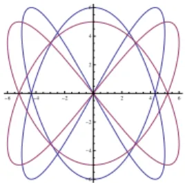
When b 6= 0, there are two subcases. (i). (x0
1, x02) = (0, 0). If (x1, x2) = (0, 0), the geodesics are closed curves.
Otherwise, there is no solution for the system (cj). In Figures 1 and 2, we assume that α = 3, β = 2, τ = 2π with several choices of c2 and c8.
-6 -4 -2 2 4 6 -6 -4 -2 2 4 6
Figure 1. closed curves with c2 = 5, c8 = 6 and c2= 6, c8= 5
-3 -2 -1 1 2 3
-2
2 4
(ii). (x0
1, x02) 6= (0, 0). Then
(ii.1), K1m and K2m are both odd integers. In this case, (x1, x2) =
−(x0 1, x02).
(ii.2), K1m and K2m are both even integers. In this case, (x1, x2) =
(x0 1, x02).
(ii.3), K1m is odd and K2m is even. In this case, (x1, x2) is the
inter-section of the lines `1 and `2. Here `1 is the line passing through the point
(−x01, −x02) with slope µ2−a
b and `2 is the line passing through (x01, x02) with
slope µ1−a
b .
(ii.4), K1m is even and K2m is odd. In this case, (x1, x2) is the
inter-section of the lines `1 and `2. Here `1 is the line passing through the point
(−x0
1, −x02) with slope µ1b−a and `2 is the line passing through (x01, x02) with
slope µ2−a b . -2 0 2 -2 0 2 1 2 3 4
Figure 3. Every point on the line has infinitely many geodesics connecting (x0 1, x02)
Assume that (x1, x2) satisfies conditions in (i) or (ii). Then
" f M1 0 β1 0 Mf2 β2 # → 1 0 0 0 ... b1 cos(√−µ1τ ) sin( √ −µ1τ ) 0 0 ... b2 0 0 1 0 ... b3 0 0 cos(√−µ2τ ) sin(√−µ2τ ) ... b4 → 1 0 0 0 ... b1 0 0 0 0 ... 0 0 0 1 0 ... b3 0 0 0 0 ... 0
Therefore, (
c1 = b1
c3 = b3
where c2 and c4 are arbitrary constants. Hence, once (cj) has a solution,
then the number of solutions is infinite with order R × R. (A.2). b2 6= (−1)K1mb
1 or b4 6= (−1)K2mb3. In this case, all cj, j = 1, 2, 3, 4
are independent. (B). τ 6= √K1
−µ1mπ, m ∈ N. In this case, det fM1 · det fM2 6= 0. Then the
system (cj) has a unique solution.
· c1 c2 ¸ = · 1 0 cos(√−µ1τ ) sin(√−µ1τ ) ¸−1· b1 b2 ¸ , · c3 c4 ¸ = · 1 0 cos(√−µ2τ ) sin( √ −µ2τ ) ¸−1· b3 b4 ¸ . 2.5.2 √√−µ1 −µ2 6∈ Q.
In this case,P2j=1¡det fMj¢26= 0. There are three subcases.
(A∗). k1 =
√ −µ1τ
π ∈ N, det fM1= 0, det fM26= 0.
(A∗.1). b
2 = (−1)k1b1. Then system (cj) has infinitely many solutions.
• When k1 is even, then (x1, x2) belongs to the line passing through the
point (x01, x02) with slope µ1−a
b . (If b = 0, the line is x1 = x01.)
• When k1 is odd, then (x1, x2) belongs to the line passing through the
point (−x0
1, −x02) with slope µ1b−a. (If b = 0, the line is x1 = −x01.) In this
case, ( c1 = b1 c2 : arbitrary and · c3 c4 ¸ = · 1 0 cos(√−µ1τ ) sin( √ −µ1τ ) ¸−1· b3 b4 ¸ .
(B∗). k2=
√ −µ2τ
π ∈ N, det fM2 = 0, det fM16= 0.
(B∗.1). b4 = (−1)k2b3. The system (cj) has infinitely many solutions.
• When k2 is even, then (x1, x2) belongs to the line passing through the point (x0
1, x02) with slope µ1b−a. (If b = 0, the line is x1 = x01.)
• When k2 is odd, then (x1, x2) belongs to the line passing through the
point (−x0
1, −x02) with slope µ1b−a. (If b = 0, the line is x1 = −x01.) In this
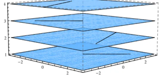
case, · c1 c2 ¸ = · 1 0 cos(√−µ1τ ) sin(√−µ1τ ) ¸−1· b1 b2 ¸ and ( c3 = b3 c4 : arbitrary -2 0 2 -2 0 2 1 2 3 4
Figure 4. Every point on the plane except a single point has no geodesics connecting (x0 1, x02)
As we can see from results for (A∗.1) and (B∗.1), the number of solutions
for the system (cj) has order R (not R × R). (B∗.3). b
4 6= (−1)k2b3. The system (cj) has no solution.
(C∗). √−µ1τ
π 6∈ N and √
−µ2τ
π 6∈ N. The system (cj) has a unique solution.
· c1 c2 ¸ = · 1 0 cos(√−µ1τ ) sin(√−µ1τ ) ¸−1· b1 b2 ¸ and · c3 c4 ¸ = · 1 0 cos(√−µ2τ ) sin(√−µ2τ ) ¸−1· b3 b4 ¸
In order to discuss geodesics which are induced by the operator L, we have the following definition.
Definition 2.1 The set of points (τ ; x1, x2) ∈ R3 in the boundary
condi-tions (2.8) such that the system (2.13) has unique solution is called regular region. The set of points (τ ; x1, x2) ∈ R3 in the boundary conditions (2.8)
such that the system (2.13) has infinitely many solutions is called Type I singular region and the set of points (τ ; x1, x2) ∈ R3 in the boundary
con-ditions (2.8) such that the system (2.13) has no solution is called Type II singular region.
For the case 5.1.1 (A), singular region is the plane Σ = {(τ, x1, x2) :
τ = √K1
−µ1mπ} in which type I singular region is a single point and the rest
of points in the plane form a type II singular region. The rest of the space is regular.
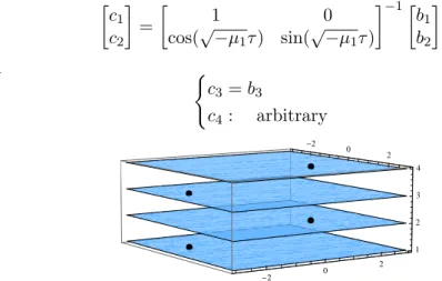
For cases 5.1.2 (A∗.1) and (B∗.1), singular region are planes Σ j =
{(τ, x1, x2) : τ = √kj
−µjmπ}, kj ∈ N. For each plane, the type I
singu-lar region is a line passing through points (x0
1, x02) or (−x01, −x02). The rest
of points in those planes form a type II singular region. The rest of the space is regular.
Moreover, one has (if b 6= 0) c5 c6 c7 c8 = µ1−a b µ1−a b µ 2−a b µ2−a b c1 c2 c3 c4 . Since µ1−a b µ 1−a b µ 2−a b µ2−a b b1 b2 b3 b4 = b µ1−µ2x 0 1+µµ11−µ−a2x 0 2 b µ1−µ2x1+ µ1−a µ1−µ2x2 −b µ1−µ2x 0 1−µµ12−µ−a2x 0 2 −b µ1−µ2x1− µ2−a µ1−µ2x2 and c2, c4 arbitrary, therefore,
c5 c6 c7 c8 = b µ1−µ2x 0 1+µ1b−ax 0 2 c0 2 −b µ1−µ2x 0 1−µ2b−ax 0 2 c0 4
calcula-2.6 Case (6). 0 > µ1 = µ2.
In this case, b = 0 and a = d = µ1 = µ2. We have
· x1(s) x2(s) ¸ = · c1 c2 c3 c4 c5 c6 c7 c8 ¸ cos(√−µ1s) sin(√−µ1s) s cos(√−µ1s) s sin(√−µ1s) . This yields · ˙x1(s) ˙x2(s) ¸ = · c1 c2 c3 c4 c5 c6 c7 c8 ¸ 0 −√−µ1 0 0 √ −µ1 0 0 0 1 0 0 −√−µ1 0 1 √−µ1 0 cos(√−µ1s) sin(√−µ1s) s cos(√−µ1s) s sin(√−µ1s) . It follows that · ¨ x1(s) ¨ x2(s) ¸ = · c1 c2 c3 c4 c5 c6 c7 c8 ¸ 0 −√−µ1 0 0 √ −µ1 0 0 0 1 0 0 −√−µ1 0 1 √−µ1 0 2 µ1cos( √ −µ1s) µ1sin(√−µ1s) µ2cos( √ −µ2s) µ2sin( √ −µ2s) .
Since ¨x = Ax, then
· c1 c2 c3 c4 c5 c6 c7 c8 ¸ µ1 0 0 0 0 µ1 0 0 0 −2√−µ1 µ1 0 −2√−µ1 0 0 µ1 = · µ1 0 0 µ1 ¸ · c1 c2 c3 c4 c5 c6 c7 c8 ¸ . This forces c3 = c4 = c7 = c8 = 0.
Using the boundary conditions (2.8), one has 1 0 0 0 cos(√−µ1τ ) sin( √ −µ1τ ) 0 0 0 0 1 0 0 0 cos(√−µ1τ ) sin( √ −µ1τ ) c1 c2 c5 c6 = x01 x1 x0 2 x2 .
2.6.1 τ = √kπ
−µ1, k ∈ N.
This case is equivalent to det · 1 0 cos(√−µ1τ ) sin( √ −µ1τ ) ¸ = sin£√−µ1τ ¤ = 0. There are two subcases.
• k is even. If (x1, x2) = (x01, x02), then the system (cj) has infinitely
many solutions. Otherwise, it has no solution.
• k is odd. If (x1, x2) = (−x01, −x02), then the system (cj) has infinitely
many solutions. Otherwise, it has no solution. When (cj) has a solution, we have
(
c1 = x01
c3 = x02
where c2 and c4 are arbitrary constants.
2.6.2 τ 6= √kπ −µ1.
This case is equivalent to det · 1 0 cos(√−µ1τ ) sin( √ −µ1τ ) ¸ = sin£√−µ1τ¤6= 0.
Then c1, c2, c3, c4 have unique solution as follows:
· c1 c2 ¸ = · 1 0 cos(√−µ1τ ) sin( √ −µ1τ ) ¸−1· x0 1 x1 ¸ , and · c5 c6 ¸ = · 1 0 cos(√−µ2τ ) sin(√−µ2τ ) ¸−1· x0 2 x2 ¸ .
2.7 Case (7). 0 = µ1 > µ2.
In this case, b = 0 and a = d = µ1 = µ2. We have
· x1(s) x2(s) ¸ = · c1 c2 c3 c4 c5 c6 c7 c8 ¸ 1 s cos(√−µ2s) sin(√−µ2s) . This yields · ˙x1(s) ˙x2(s) ¸ = · c1 c2 c3 c4 c5 c6 c7 c8 ¸ 0 0 0 0 0 1 0 0 0 0 −√−µ2 0 0 0 0 √−µ1 1 1 cos(√−µ2s) sin(√−µ2s) . It follows that · ¨ x1(s) ¨ x2(s) ¸ = · c1 c2 c3 c4 c5 c6 c7 c8 ¸ 0 0 0 0 0 0 0 0 0 0 µ2 0 0 0 0 µ2 1 s cos(√−µ2s) sin(√−µ2s) .
Since ¨x = Ax, then (if b 6= 0)
c5 c6 c7 c8 = −a b −ab µ2−a b µ2−a b c1 c2 c3 c4 .
Using the boundary conditions (2.8), we may come up a system for cj’s,
j = 1, . . . , 8 as follows: M10 0 ... β1 0 M20 ... β2 . Here M10 = · 1 0 1 τ ¸ , M20 = · 1 0 cos(√−µ2τ ) sin( √ −µ2τ ) ¸ and β1 = · b1 b2 ¸ , β2 = · b3 b4 ¸
with b1= µ2µ−a2 x01−µb2x 0 2 b2= µ2µ−a2 x1−µb2x2 b3= µa2x01+µb2x 0 2 b4= µa2x1−µb2x2
This implies that · c1 c2 ¸ = · 1 0 1 τ ¸−1· b1 b2 ¸ = 1 τ · τ 0 −1 1 ¸ · b1 b2 ¸ .
Now we need to find c3 and c4. There are two subcases.
2.7.1 det M0 2= 0. In this case, k2= √ −µ2τ π ∈ N. Then • b4= (−1)k2b3 which is equivalent to x1−x01 x2−x02 = − b a, when k2 is even x1−(−x01) x2−(−x02) = − b a, when k2 is odd
Then the system (cj) has infinitely many solutions. Therefore, (
c3 = b3
c4 : arbitrary
• b46= (−1)k2b
3. Then (cj) has no solution.
2.7.2 det M20 6= 0.
In this case, √−µ2τ
π 6∈ N. Then c3 and c4 have unique solution:
· c3 c4 ¸ = · 1 0 cos(√−µ2τ ) sin( √ −µ2τ ) ¸−1· b3 b4 ¸ .
2.8 Case (8). µ1 > 0 > µ2. We have · x1(s) x2(s) ¸ = · c1 c2 c3 c4 c5 c6 c7 c8 ¸ e−√µ1s e√µ1s cos(√−µ2s) sin(√−µ2s) . This yields · ¨ x1(s) ¨ x2(s) ¸ = · c1 c2 c3 c4 c5 c6 c7 c8 ¸ µ1e− √ µ1s µ1e−√µ1s µ2cos( √ −µ2s) µ2sin(√−µ2s) .
Since ¨x = Ax, then (if b 6= 0)
c5 c6 c7 c8 = µ1−a b µ1−a b µ2−a b µ 2−a b c1 c2 c3 c4 .
Using the boundary conditions (2.8), we may come up a system for cj’s,
j = 1, . . . , 8 as follows:
M1 0 ... β1
0 Mf2 ... β2
. Here the matrices M1 and fM2 are defined as before:
M1 = · 1 1 e−√µ1τ e√µ1τ ¸ , Mf2= · 1 0 cos(√−µ2τ ) sin(√−µ2τ ) ¸ and β1 = · b1 b2 ¸ , β2 = · b3 b4 ¸ with b1 = µa−µ1−µ22x01+ µ1−µb 2x 0 2 b2 = µa−µ1−µ22x1+ µ1−µb 2x2 b3 = µ1a−ax01− µ1−µb 2x 0 2 b4 = µ1a−ax1− µ1−µb 2x2
This implies that · c1 c2 ¸ = · 1 1 e−√µ1τ e√µ1τ ¸−1· b1 b2 ¸ .
There are two subcases.
2.8.1 det fM2= 0. In this case, k2= √ −µ2τ π ∈ N. Then • b4= (−1)k2b3 which is equivalent to x1−x01 x2−x02 = b
µ1−a, when k2 is even
x1−(−x01)
x2−(−x02) =
b
µ1−a, when k2 is odd
Therefore, the system (cj) has infinitely many solutions. It follows that
(
c3 = b3
c4 : arbitrary
• b46= (−1)k2b3. Then the system (cj) has no solution.
2.8.2 det fM26= 0.
In this case, √−µ2τ
π 6∈ N. Then c3 and c4 have the following form:
· c3 c4 ¸ = · 1 0 cos(√−µ2τ ) sin( √ −µ2τ ) ¸−1· b3 b4 ¸ ,
3
Action functions
Form results in section 1, we know that solutions (geodesics) for Hamiltonian system are determined by the eigenvalues of the matrix A = B + Bt. More
precisely, we know that
• If A is positive definite or positive semi-definite, geodesic is unique. • If A is negative definite or negative semi-definite, then the number of
geodesics relies on the choices of the initial conditions. It maybe has unique, infinitely many or even none geodesic.
Now we are going to use energy to obtain action functions corresponding to different situations for A. In the rest of this section, the matrix P = CtC
plays an important role, i.e., p11 p12 p13 p14 p21 p22 p23 p24 p31 p32 p33 p34 p41 p42 p43 p44 = c1 c5 c2 c6 c3 c7 c4 c8 · c1 c2 c3 c4 c5 c6 c7 c8 ¸ = c2 1+ c25 c1c2+ c5c6 c1c3+ c5c7 c1c4+ c5c8 c1c2+ c5c6 c22+ c26 c2c3+ c6c7 c2c4+ c6c8 c1c3+ c5c7 c2c3+ c6c7 c23+ c27 c3c4+ c7c8 c1c4+ c5c8 c2c4+ c6c8 c3c4+ c7c8 c24+ c28 (3.15)
Observe the submatrix · p13 p14 p23 p24 ¸ = · c1c3+ c5c7 c1c4+ c5c8 c2c3+ c6c7 c2c4+ c6c8 ¸ = · c1 c2 ¸ £ c3 c4¤+ · c5 c6 ¸ £ c7 c8¤. When b 6= 0, · c5 c6 ¸ = µ1− a b · c1 c2 ¸ , · c7 c8 ¸ = µ2− a b · c3 c4 ¸ and 1 +(µ1− a)(µ2− a) b2 = µ1µ2− a(µ1+ µ2) + a2+ b2 b2 =ad − b2− a(a + d) + a2+ b2 b2 = 0.
It follows that the matrix P can be written as P = p11 p12 0 0 p12 p22 0 0 0 0 p33 p34 0 0 p34 p44 .
The energy E can be obtained from geodesics. In fact, ¨ x = Ax ⇒ 2h ˙x, ¨xi = 2h ˙x, Axi ⇒ d dsh ˙x, ˙xi = d dshx, Axi ⇒ h ˙x, ˙xi − hx, Axi = 2E therefore, E = 1 2 ¡ h ˙x, ˙xi − hx, ¨xi¢.
Following results from Section 1, there are 8 different cases.
3.1 Case (1). µ1 > µ2 > 0. Denote U = · u11 u12 u21 u22 ¸ = · 1 1 e−√µ1τ e√µ1τ ¸−1 = 1 2 sinh√µ1τ · e√µ1τ −1 −e−√µ1τ 1 ¸ (3.16) and V = · v11 v12 v21 v22 ¸ = · 1 1 e−√µ2τ e√µ2τ ¸−1 = 1 2 sinh√µ2τ · e√µ2τ −1 −e−√µ2τ 1 ¸ . (3.17) It follows that · c1 c2 ¸ =U · " a−µ2 µ1−µ2x 0 1+µ1−µb 2x 0 2 a−µ2 µ1−µ2x1+ b µ1−µ2x2 # " ¡ ¢ √ ¡ ¢ #
· c3 c4 ¸ =V · " µ1−a µ1−µ2x 0 1−µ1−µb 2x 0 2 µ1−a µ1−µ2x1− b µ1−µ2x2 # = 1 2 sinh√µ2τ " ¡ µ 1−a µ1−µ2x 0 1−µ1−µb 2x 0 2 ¢ e√µ2τ −¡µ1−a µ1−µ2x1− b µ1−µ2x2 ¢ 1 −¡µ1−a µ1−µ2x 0 1−µ1−µb 2x 0 2 ¢ e−√µ2τ+¡µ1−a µ1−µ2x1− b µ1−µ2x2 ¢ 1 # ; · c5 c6 ¸ =U · " b µ1−µ2x 0 1+µµ11−µ−a2x 0 2 b µ1−µ2x1+ µ1−a µ1−µ2x2 # = 1 2 sinh√µ1τ " ¡ b µ1−µ2x 0 1+µµ11−µ−a2x 0 2 ¢ e√µ1τ −¡ b µ1−µ2x1+ µ1−a µ1−µ2x2 ¢ 1 −¡ b µ1−µ2x 0 1+µµ11−µ−a2x 0 2 ¢ e−√µ1τ+¡ b µ1−µ2x1+ µ1−a µ1−µ2x2 ¢ 1 # ; and · c7 c8 ¸ =V · " −b µ1−µ2x 0 1+µa−µ1−µ22x 0 2 −b µ1−µ2x1+ a−µ2 µ1−µ2x2 # = 1 2 sinh√µ2τ " ¡ −b µ1−µ2x 0 1+ µa−µ2−µ21x 0 2 ¢ e√µ2τ+¡ b µ1−µ2x1− a−µ2 µ1−µ2x2 ¢ 1 ¡ b µ1−µ2x 0 1− µa−µ1−µ22x 0 2 ¢ e−√µ2τ+¡ −b µ1−µ2x1+ a−µ2 µ1−µ2x2 ¢ 1 # . Hence, · x1(s) x2(s) ¸ = · c1 c2 c3 c4 c5 c6 c7 c8 ¸ e−√µ1s e√µ1s e−√µ2s e√µ2s = · c1e− √ µ1s+ c 2e √ µ1s+ c 3e− √ µ2s+ c 4e √ µ2s c5e− √µ 1s+ c 6e √µ 1s+ c 7e− √µ 2s+ c 8e √µ 2s ¸ . It follows that · ˙x1(s) ˙x2(s) ¸ = · c1 c2 c3 c4 c5 c6 c7 c8 ¸ −√µ1e− √ µ1s √ µ1e √µ 1s −√µ2e− √ µ2s √ µ2e √µ 2s and · ¨ x1(s) ¨ x2(s) ¸ = · c1 c2 c3 c4 c5 c6 c7 c8 ¸ µ1e−√µ1s µ1e √ µ1s µ2e− √µ 2s µ2e √ µ2s .
Therefore, h ˙x(s), ˙x(s)i = −√µ1e− √µ 1s √ µ1e √µ 1s −√µ2e− √ µ2s √ µ2e√µ2s t p11 p12 0 0 p12 p22 0 0 0 0 p33 p34 0 0 p34 p44 −√µ1e− √µ 1s √ µ1e √µ 1s −√µ2e− √ µ2s √ µ2e√µ2s = D −√µ1e− √ µ1sp 11+√µ1e √ µ1sp 12 −√µ1e−√µ1sp 12+√µ1e √µ 1sp 22 −√µ2e− √ µ2sp 33+√µ2e √ µ2sp 34 −√µ2e− √µ 2sp 34+√µ2e √µ 2sp 44 , −√µ1e− √ µ1s √ µ1e√µ1s −√µ2e− √ µ2s √ µ2e √µ 2s E = 1 1 1 1 t µ1e−2√µ1sp 11 −µ1p12 0 0 −µ1p12 µ1e2 √ µ1sp 22 0 0 0 0 µ2e−2√µ2sp 33 −µ2p34 0 0 −µ2p34 µ2e2 √ µ2sp 44 1 1 1 1
Similarly, one has
hx(s), ¨x(s)i = e−√µ1s e√µ1s e−√µ2s e√µ2s t p11 p12 0 0 p12 p22 0 0 0 0 p33 p34 0 0 p34 p44 µ1e− √µ 1s µ1e √µ 1s µ2e− √ µ2s µ2e√µ2s = 1 1 1 1 t µ1e−2 √ µ1sp 11 µ1p12 0 0 µ1p12 µ1e2 √µ 1sp 22 0 0 0 0 µ2e−2 √ µ2sp 33 µ2p34 0 0 µ2p34 µ2e2 √ µ2sp 44 1 1 1 1
Therefore, the energy E can be calculated as follows
E =1 2 ³ h ˙x(s), ˙x(s)i − hx(s), ¨x(s)i ´ =1 2 1 1 1 1 t 0 −2µ1p12 0 0 −2µ1p12 0 0 0 0 0 0 −2µ2p34 0 0 −2µ2p34 0 1 1 1 1 = − 2¡µ1p12+ µ2p34 ¢ .
Now we need to calculate p12 and p34. In order to do that, From (3.15), we need to calculate c1c2 and c5c6. From results above, we know that
c1c2 = h¡ a − µ2 µ1− µ2x 0 1+ b µ1− µ2x 0 2 ¢ u11+ ¡ a − µ2 µ1− µ2x1+ b µ1− µ2x2 ¢ u12 i ×h¡ a − µ2 µ1− µ2 x01+ b µ1− µ2 x02¢u21+¡ a − µ2 µ1− µ2 x1+ b µ1− µ2 x2¢u22 i =¡ a − µ2 µ1− µ2 x01+ b µ1− µ2 x02¢2u11u21 +¡ a − µ2 µ1− µ2x 0 1+ b µ1− µ2x 0 2 ¢¡ a − µ2 µ1− µ2x1+ b µ1− µ2x2 ¢ (u11u22+ u12u21) +¡ a − µ2 µ1− µ2x1+ b µ1− µ2x2 ¢2 u12u22; (3.18) and c5c6 =h¡ b µ1− µ2 x01+ µ1− a µ1− µ2 x02¢u11+¡ b µ1− µ2 x1+ µ1− a µ1− µ2 x2¢u12 i ×h¡ b µ1− µ2x 0 1+ µ1− a µ1− µ2x 0 2 ¢ u21+ ¡ b µ1− µ2x1+ µ1− a µ1− µ2x2 ¢ u22 i =¡ b µ1− µ2x 0 1+ µ1− a µ1− µ2x 0 2 ¢2 u11u21 +¡ b µ1− µ2x 0 1+ µ1− a µ1− µ2x 0 2 ¢¡ b µ1− µ2x1+ µ1− a µ1− µ2x2 ¢ (u11u22+ u12u21) +¡ b µ1− µ2x1+ µ1− a µ1− µ2x2 ¢2 u12u22. (3.19) Plugging (3.16) into (3.18) and (3.19), one has
p12= c1c2+ c5c6 = R21 cosh√µ1τ sinh2√µ1τ −R2 4 1 sinh2√µ1τ where R1 =³ a − µ2 µ1− µ2 x01+ b µ1− µ2 x02´³ a − µ2 µ1− µ2 x1+ b µ1− µ2 x2 ´ + ³ b µ1− µ2 x1+ µ1− a µ1− µ2 x2 ´³ b µ1− µ2 x01+ µ1− a µ1− µ2 x02 ´ R2 =³ a − µµ 2 1− µ2 x01+ b µ1− µ2x 0 2 ´2 + ³ b µ1− µ2x 0 1+ µ1− a µ1− µ2x 0 2 ´2 +³ a − µ2 µ − µ x1+ b µ − µ x2 ´2 + ³ b µ − µ x1+ µ1− a µ − µ x2 ´2 .
Similarly, p34= c3c4+ c7c8 = R23 cosh√µ2τ sinh2√µ2τ −R4 4 1 sinh2√µ2τ where R3 =³ a − µµ 1 1− µ2x 0 1+ b µ1− µ2x 0 2 ´³ a − µ1 µ1− µ2x1+ b µ1− µ2x2 ´ + ³ b µ1− µ2x 0 1+ µ2− a µ1− µ2x 0 2 ´³ b µ1− µ2x1+ µ2− a µ1− µ2x2 ´ R4 =³ µ1− a µ1− µ2 x01− b µ1− µ2 x02 ´2 + ³ b µ1− µ2 x01+ µ2− a µ1− µ2 x02 ´2 +³ a − µ1 µ1− µ2x1+ b µ1− µ2x2 ´2 + ³ b µ1− µ2x1+ µ2− a µ1− µ2x2 ´2 .
Therefore, the action function S is
S = − Z Edτ = 2µ1 Z p12dτ + 2µ2 Z p34dτ =µ1R1 Z cosh√µ1τ sinh2√µ1τ dτ − µ1R2 2 Z dτ sinh2√µ1τ + µ2R3 Z cosh√µ2τ sinh2√µ2τ dτ − µ2R4 2 Z dτ sinh2√µ2τ = − √ µ1R1 sinh√µ1τ + √ µ1R2 2 coth √ µ1τ − √ µ2R3 sinh√µ2τ + √ µ2R4 2 coth √ µ2τ. 3.2 Case (2). µ1 = µ2 > 0. In this case, · c1 c2 ¸ = U · · x0 1 x1 ¸ = 1 2 sinh√µ1τ · e√µ1τx0 1− x1 −e−√µ1τx0 1+ x1 ¸ ; (3.20) and
It follows that · x1(s) x2(s) ¸ = · c1 c2 c5 c6 ¸ · e−√µ1s e√µ1s ¸ = · c1e− √ µ1s+ c 2e √ µ1s c5e−√µ1s+ c 6e √µ 1s ¸ . Hence, · ˙x1(s) ˙x2(s) ¸ = · c1 c2 c5 c6 ¸ · −√µ1e− √µ 1s √ µ1e √ µ1s ¸ and · ¨ x1(s) ¨ x2(s) ¸ = · c1 c2 c5 c6 ¸ · µ1e− √µ 1s µ1e √µ 1s ¸ .
This implies that
h ˙x(s), ˙x(s)i = · −√µ1e− √ µ1s √ µ1e√µ1s ¸t· p11 p12 p12 p22 ¸ · −√µ1e− √ µ1s √ µ1e√µ1s ¸ = · 1 1 ¸t· µ1e−2 √µ 1sp 11 −µ1p12 −µ1p12 µ1e2 √ µ1sp 22 ¸ · 1 1 ¸ and hx(s), ¨x(s)i = · e−√µ1s e√µ1s ¸t· p11 p12 p12 p22 ¸ · µ1e− √µ 1s µ1e √ µ1s ¸ = · 1 1 ¸t· µ1e−2 √ µ1sp 11 µ1p12 µ1p12 µ1e2√µ1sp 22 ¸ · 1 1 ¸ . One has h ˙x(s), ˙x(s)i − hx(s), ¨x(s)i = · 1 1 ¸t· 0 −2µ1p12 −2µ1p12 0 ¸ · 1 1 ¸ = −4µ1p12.
Now we just need to calculate p12. It reduces to calculate c1c2 and c5c6.
From (3.22) and (3.23), we know that
c1c2 = (x01)2u11u21+ x01x1(u11u22+ u12u21) + x21u12u22; (3.22)
and
Using results (3.22) and (3.23), one has p12=c1c2+ c5c6 =£(x01)2+ (x20)2¤u11u21+ ¡ x01x1+ x02x2 ¢ (u11u22+ u12u21) + ¡ x21+ x22¢u12u22 =kx0k2u11u21+ ¡ x0· x ¢ (u11u22+ u12u21) + kxk2u12u22 =1 2(x0· x) cosh√µ1τ sinh2√µ1τ −1 4(kx0k 2+ kxk2) 1 sinh2√µ1τ .
Hence, the energy E has the following form
E =1 2 ¡ h ˙x, ˙xi − hx, ¨xi¢= −2µ1p12 = − µ1(x0· x) cosh√µ1τ sinh2√µ 1τ +µ1 2 (kx0k 2+ kxk2) 1 sinh2√µ 1τ .
It follow that the action function S is
S = − Z Edτ = − √ µ1(x0· x) sinh√µ1τ + √ µ1(kx0k2+ kxk2) 2 coth √ µ1τ. Here x0 = [x0
1, x02]t and x = [x1, x2]t. As usual, x0· x = x01x1 + x02x2 and
kx0k2+ kxk2 = (x01)2+ (x02)2+ x21+ x22. 3.3 Case (3). µ1 > µ2 = 0. In this case, · c1 c2 ¸ =U · " a µ1x 0 1+ µb1x 0 2 a µ1x1+ b µ1x2 # = 1 2 sinh√µ1τ " ¡ a µ1x 0 1+µb1x 0 2 ¢ e√µ1τ−¡a µ1x1+ b µ1x2 ¢ −¡µa1x0 1+µb1x 0 2 ¢ e−√µ1τ −¡a µ1x1+ b µ1x2 ¢ # ; (3.24) · c3 c4 ¸ = · 1 0 1 τ ¸−1"µ1−a µ1 x 0 1−µb1x 0 2 µ1−a µ1 x1− b µ1x2 # " ¡ ¢ # (3.25)
· c5 c6 ¸ =U · " b µ1x 0 1+ µ1µ−a1 x 0 2 b µ1x1+ µ1−a µ1 x2 # = 1 2 sinh√µ1τ " ¡ a µ1x 0 1+µb1x 0 2 ¢ e√µ1τ−¡a µ1x1+ b µ1x2 ¢ −¡µa 1x 0 1+µb1x 0 2 ¢ e−√µ1τ −¡a µ1x1+ b µ1x2 ¢ # ; (3.26) and · c7 c8 ¸ = · 1 0 1 τ ¸−1" −µb1x0 1+µa1x 0 2 −µb1x1+µa1x2 # =1 τ " ¡ −µb1x0 1+µa1x 0 2 ¢ τ ¡ b µ1x 0 1−µa1x 0 2 ¢ −¡µb1x1−µa1x2 ¢ # ; (3.27) It follows that · x1(s) x2(s) ¸ = · c1 c2 c3 c4 c5 c6 c6 c7 ¸ e−√µ1s e√µ1s 1 s = · c1e−√µ1s+ c 2e √µ 1s+ c 3+ c4s c5e− √ µ1s+ c 6e √ µ1s+ c 7+ c8s ¸ . Hence, · ˙x1(s) ˙x2(s) ¸ = · c1 c2 c3 c4 c5 c6 c7 c8 ¸ −√µ1e− √ µ1s √ µ1e √µ 1s 0 1 and · ¨ x1(s) ¨ x2(s) ¸ = · c1 c2 c3 c4 c5 c6 c7 c8 ¸ µ1e− √ µ1s µ1e √µ 1s 0 0 .