Vehicle-type motion estimation by the fusion of image point and line features

(1)

Pergamon

PII: S0031-3203 (97) 00044-7

V E H I C L E - T Y P E M O T I O N E S T I M A T I O N BY T H E F U S I O N

O F I M A G E P O I N T A N D L I N E F E A T U R E S

SOO-CHANG PEI* and L I N - G W O LIOU

Department of Electrical Engineering, National Taiwan University, Taipei, Taiwan, R.O.C. (Received 14 November 1994; received for publication 7 April 1997)

Abstract--Three-dimensional (3D) motion estimation is a very important topic in machine vision. How- ever, reliability of the estimated 3D motion seems to be the most challenging problem, especially to the linear algorithms developed for solving a general 3D motion problem (six degrees of freedom). In real applications such as the traffic surveillance and auto-vehicle systems, the observed 3D motion has only three degrees of freedom because of the ground plane constraint (GPC). In this paper, a new iterative method is proposed for solving the above problem. Our method has several advantages: (1) It can handle both the point and line features as its input image data. (2) It is very suitable for parallel processing. (3) Its cost function is so well-conditioned that the final 3D motion estimation is robust and insensitive to noise, which is proved by experiments. (4) It can handle the case of missing data to a certain degree. The above benefits make our method suitable for a real application. Experiments including simulated and real-world images show satisfactory results. © 1997 Pattern Recognition Society. Published by Elsevier Science Ltd. Image points Image lines Traffic surveillance system Ground plane constraint

l. INTRODUCTION

The problem of estimating 3D motion/structure parameters from an image sequence has been the focus of a significant amount of research during the past years. In several industrial applications, the ability to per- form detection and estimation of motion has become a basic task of the robotic vision system. The difficulty of motion analysis may be broken into two parts: (1) measurement--to extract image features and measure their 2D motions on the image plane. (2) 3D motion estimation--from the above 2D measurements to estimate 3D motion and infer the object structure. The second part is the main concern of this paper.

To solve the above 3D motion estimation problem, the so-called correspondence approaches are often utilized. They analyze discrete motion measurement of the same physical features (points, lines .. . . . etc.) over time. Besides, they often assume that the 3D motion of the target is rigid. By the image features and strategies they used, we briefly describe these techniques.

Roach and Aggarwal m proposed an algorithm of 3D motion estimation using point correspondences. It is based on the distance invariance of the points of a 3D rigid object. This method is nonlinear and therefore initial guesses or global search have to be adopted. Besides, several linear algorithms were proposed. Examples include Longuet-Higgins, t2J Tsai and Huang, t3) Zhuang, t4) Weng and Huang, 15) Phi- lip, t6) and Spetsakis and AloimonosF ) The main step of these linear algorithms is to solve an intermediate

matrix linearly from point correspondences. Then the motion parameters will be determined by decompos- ing this intermediate matrix. These linear methods need at least eight point correspondences at two views and they are sensitive to noise. Several methods about point tracking are listed in references (8-11).

Compared with the point features, the line features have better performance in the reliability of measurement. Measurement of a line feature can easily achieve the sub-pixel accuracy. However, a line feature reveals less 3D motion clues than that from a point feature. So it often needs more sets of line correspondences in more views (than points) to solve a 3D motion problem. The algorithm proposed by Yen and Huang ~12) is based on projecting image lines on a unit sphere; the 3D rotations are estimated iteratively from line correspondences over three frames. Mitichi, Seida and Aggarwal ~1 a) used angle invariance of any two lines of a 3D rigid object; this algorithm used rigidity constraint to reconstruct the 3D lines and then computes the 3D motion parameters. Lately, linear algorithms for lines are proposed. Their basic derivations are very similar to that for points. Examples include Liu and Huang, t14-as) Spetsakis and Aloimonos, I16) Weng, Huang and Ahuja. t~7) These linear algorithms need at least 13-line correspondences at three views and they are very sensitive to noise. Some methods about tracking a line feature are listed in references (18-21). In industrial applications, reliability of an algorithm should be highly considered. To achieve high robustness, three possible strategies were often utilized.

• To use long image sequence and local smoothness *Author to whom correspondence should be addressed. 3D motion constraint. Examples include Broida

(2)

334 SOO-CHANG PEI and LIN-GWO LIOU

and Chellappa, 122~ Weng, Huang and Ahuja,/23) Tseng and Sood, ~24) Shariat and Price, ~25) and Broida and Chellappa, ~26) and Hu and Ahuja. ~27~ Most of them used point correspondences only. • To use as many available image features as

possible. For example, Wang, Karandikar and AggarwaP TM and Liu, Huang and Faugeras ~29J con-

sidered the use of both image point and line features as their input.

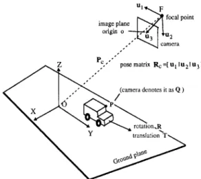
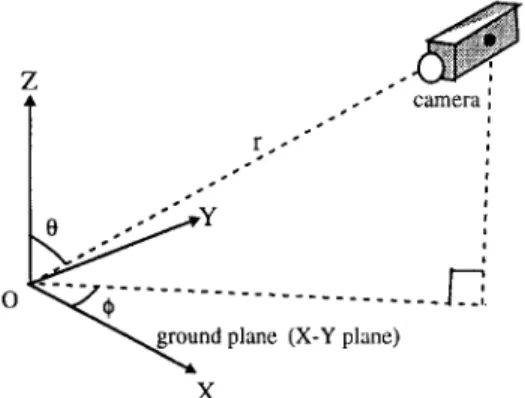
• To use additional physical constraints in some special applications. Nonlinearity of the motion analysis will be greatly simplified, and the number of unknowns will be reduced. Examples include the ground plane constraint (GPC) in the traffic surveillance system or the auto-navigation system (see Fig. 1). ~30'31)

Inspired by the above ideas, a new iterative algorithm is proposed in this paper. It considers a special vehicle-type motion problem. A closed-form solution is also derived as an initial estimate to our algorithm. This initial solution is precisely accurate when no errors exist.

Our algorithm has several important properties: (1) Both the image points and lines can be accepted as the input of the algorithm. (2) It minimizes a 2D cost function to find the optimum solution. (3) The definition of the cost function is especially taken care such that the cost function is well-shaped (or well-conditioned). (4) It is very suitable for parallel processing. (5) Our algorithm can be easily extended to a long image sequence and it can handle missing data to a certain degree.

To complete the algorithm, several important issues are discussed: (1) Weighting problem. (2) The smallest number of required image features. (3) The case when no rotation exists. Experiments, including both the simulated and real-world image tests, prove the correctness and robustness of this algorithm.

To stress the difference between our iterative method and the traditional linear one [especially to the Spetsakis's method~33)], both of them are compared in the following directions:

• Technique. Basically, the linear method is indirect. No matter how the motion type is constrained, 27 intermediate variables should be first solved any- way. It means that we should use more redundant image features than that required (and even larger for the robustness of solution). Finally, the 27 intermediate variables are still be sent to a nonlinear optimization process for further refinement. On the contrary, our method is a direct one. We do not have to solve the intermediate variables; therefore, the redundant image features are not so badly required.

• Accuracy. Of no doubt, solution to the intermedi-

ate variables will be very error-sensitive for ignor- ing the nonlinear constraints among them. Besides, finding the best-fit motion parameters to minimize

the residual errors of the 27 intermediate variables is not a very good idea. Constructing a good optimization criterion needs to consider the noise model of image features and the balance of weighting. The linear method never mentioned about that. On the contrary, in the vehicle-type motion problem, our method does consider all of the above factors. Practical use. In the vehicle-type 3D motion problem, our method only needs to search a two-variable cost function (about rotation). The linear method may have a large advantage in the theoretical analysis of general 3D-motion problem, but it may be not the most appropriate method for the vehicle-type 3D motion estimation.

On the whole, we can say: "The linear method is designed for speed improvement and theoretical analysis, but ours is designed for accuracy improvement and real application ".

The remainder of this paper is organized as follows: Section 2, describe several basic transform relation- ships between the camera coordinate system and the global coordinate system. Section 3, problem formulation. Section 4, description of the main algorithm. Section 5, discussions about several related problems of the algorithm. Section 6, experiments including simulated and real-world image. Section 7, final conclusion.

2. C O O R D I N A T E TRANSFORM

Without loss of generality, let us consider a traffic surveillance system shown in Fig. 1. There are two coordinate systems: ground plane coordinate system (GPCS) and camera coordinate system (CCS). The origin O of G P C S is just lying on this plane. {i, ~, ~} forms an orthonormal basis of GPCS, and the first two orthonormal vectors ( i and y) span the whole ground plane. The third unit vector ~ is then the normal vector of the ground plane. For convenience, the G P C S is considered as the global coordinate system in this paper. The camera is placed at a suitable position such that it can see the objects moving on the ground plane. The origin F of CCS is positioned at Pc - (Pox, PcY, Pcz) T (relative to GPCS). Its three orthonormal vectors, {ul, u2, u3}, specify the pose of the camera, u3 is the camera's main axis; focal length F o is set to 1; Ul and u2 are the two directions of the image axes.

A point in 3D space is separately denoted by P and Q in G P C S and CCS. We can easily derive the coordinate transform relationship between GPCS and CCS as follows:

P = RcQ + Pc or Q = a f ( P - Pc), (1)

where the matrix Rc is an orthonormal matrix and defined as

(3)

Vehicle-type motion estimation by the fusion of image point and line features 335

u,....y_

t ' ~ .~,~ focal point image plane I , " ~ 1 orJ.gin o ----p~, ~ I 'IU • 2

/

~ , , , , ~ , P c , " posematfix Rc=[UllU21U 3] " ~ ~ , - - - ~ rotation.R ' translation T ~

Fig. 1. Configuration of a traffic surveillance system.

Assume that the vehicle-type motion is specified by a rotation matrix R and a translation vector T like this

P' = R P + T, (3)

3. PROBLEM FORMULATION

Let us consider the m o n o c u l a r traffic surveillance system shown in Fig. 1. We assume that the image point and line features corresponding to a 3D moving vehicle can be continuously tracked at three image frames (t = - i, t = 0, t = + 1). Figure 2 shows the definitions for m o t i o n parameters: o)_ and T for time instants 0 and - 1; co+ and T+ for time instants 0 and + 1. The pose Rc and position Pc of the camera has been known as prior information. The camera obeys the rule of perspective projection.

N o w the question is: "How to determine the un- known 30 motion parameters [o) , o)+, T _ , T+ } from the input image data?"

Before leaving this section, we briefly explain why we need three frames to solve this problem. To the image point features, two frames are just enough for the 3D m o t i o n estimation; however, it takes at least three for the image line features to do the same thing. In order to fuse the contributions from both image points and lines, three image frames are grouped together and considered as a basic processing unit in our method. where

o'C°S snail

R = | s i n ~ o coso) - T = r • 0 (4)

The same 3D m o t i o n observed by the camera (denoted by "*") can be represented by

Q' = R * Q + T*. (5)

R* and T* also have the following special forms:

R* = R~RRc; T * = ctm~ + flmr, (6)

where mx -= R~X~, m r - R~Xy, mz - R ~ , and ot - P c x ( - 1 + cos o~) - Per s i n o + Tx; fi =- Pcx(sin@ 4- Per( - 1 4- cos oJ) 4- Tr. (7) F o r a simpler form in derivation, T* can be rewrit- ten as I-from equation (6)]

T* = [mxlmy] = Ma,

(8)

where M is a 3 × 2 matrix and a is a 2 × 1 vector. The above equations define the transform relation- ships between G P C S and CCS. The three m o t i o n parameters ~o, Tx, and Ty defined in G P C S are directly related to the m o v i n g velocity of the 3D object along the ground plane (road). In fact, with a minor modification, the above equations are also suitable for the auto-navgation system.

4. MAIN ALGORITHM

To present our m e t h o d in an organized form, we divide its derivations into the following six subsec- tions (4.1 4.6):

4.1. Definition of a general cost Junction

The purpose of our algorithm is to find the opti- m u m 3D m o t i o n parmeters which can minimize the value of a given cost function J. Assume that we have tracked Np image points and N~ image lines in three frames. Therefore, the cost function J must be divided into two parts: one for the point features, and one for the line features. It can be defined as

Nv N~

J =-- E Jp, i 4- E Ji,j,

(9)

i = l j = l

where the subscripts p and l separately represent "point" and "line" features. If three is no available image line feature (or points) in the input data, we may neglect all of the cost terms Jr.is (or Jp. is). There- fore, the definition of cost function in equation (9) is very flexible.

4.2. Cost function for image points

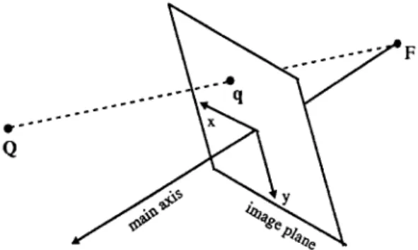
Here we will define the cost function ,lv.i for i = 1 to Np. To simplify the notations, the subscript i is temporarily neglected in the following derivation. Let us consider Fig. 3. A moving-feature point Q in 3D space is separately denoted by Q _ , Qo, and Q+ at the three interested time instants t = - l, t = 0, and t = + 1. F o r the purpose of proper weighting (explained later), their projected image points are represented by three

(4)

co_ T_ co+ T+

® ,

®

, ®

t=- 1 t=0 t=+ 1

Fig. 2. Definition of motion parameters at three time instants.

Q

y

~

F

Fig. 3. Perspective projection for a point feature.

unit vectors q , qo, and q+ (from Ix, y, 1] T to [x,

y, 1]/~/x 2 +

y2 + I).

U n d e r the perspective projection, it is easy to ob- serve that Qk (k = - , O, + ) and its projection qk are of the same direction. So the cost function Jp can be defined as

Jp = Wp{Hq- × Q - I I 2 + Ilqo × Qoql 2 + IIq+ ×Q+112},

(10)

where wp (subscript "p" denotes "point") is a weighting factor. The operator " × " denotes the outer product of vectors.

According to equations (5), (6) and (8), we have Q - = R * - Q o + T * - ; Q+ = R * Q o + T * , (11) where T* = Mak (k = - , +).

Therefore, J , is in fact a function of co , ~o +, a , a +, and Qo. To minimize Jp, we substitute equation (11) into equation (10) and set OJp/~3Qo to zero. An opti- m u m Qo can be solved in terms of a given set of motion parameters Qo = (ATA) - 1AXb, (12) where

FE a 1

A ~ x / ~ p Eo ; b~- - x / ~ p 7 . (13) [ E + R * J [ E + M a + / The matrix Ek (k = - , 0, + ) is defined as

Ek =-- qk, z 0 -- k,x •

-- qk,r qk.x

(14)

When substituting the best Qo in equation (12) into the cost function Jp, we have

Jp = bT(l -- A ( A r A ) - IAT)b -= b~Db. (15) Notice that the matrix D only depends on the un- k n o w n rotation parameters, ~,J_ and ~9+.

For a simpler mathematical form, the vector b can be rearranged as

b = - ~ p p a+

E + M

= Ha. (16)

Here H is a 9 × 4 matrix, and it depends only on the input image data; a is a 4 × 1 vector.

Substituting equation (16) into equation (15), we have

Jv = aT(HTDH)a

-aTCpa.

(17) Two things are obvious: (1) the 4 x 4 symmetric matrix Cp is a function of only two unknowns, e~_ and ~o+; (2) the cost function J , is a quadratic form of a. Each set of the corresponding image points can provide a cost function like equation (17). Adding these cost functions together, we have the final form

Jp.i = a~ Cp.i(co ,~J.,+) a = aXBpa. (18)

i = 1 i

4.3. Cost function Jor image lines

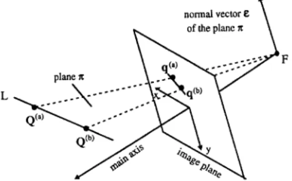
Here we will define the cost function Jt.j forj = 1 to N~. The subscriptj is also neglected for simplifying the notations. Let us consider Fig. 4. A moving feature line L in 3D space is separately denoted by L_, Lo, and L+ at the three interested time instants t = - 1, t = 0, and t = + 1. Their projected image lines are separately denoted by lkS (k = - , 0, + ). The corre- sponding 3D points on the feature lines are denoted by QkS. Each image line Ik can be represented by a unit vector ek illustrated in Fig. 4. ~:k is just defined as the normal vector of the plane ~z which passes through the focal point F and the image line lk. Obviously, ~:k is orthogonal to every point on the 3D feature line Lk. To define the cost function Jr, we appropriately choose two virtual points, say q{o ") and q~o b), on an image line lo. F o r the purpose of proper weighting, the norms of q~o a) and q~o bl are also re-scaled to 1 just as in Section 4.2. The points on the line Lo which are corresponding to the two virtual points on lo are denoted by Q~o ") and Q~). Their corresponding points at other time instants (t = - 1, 0, + 1) are then denoted by Q~") and Q~b), where k = - , 0, + .

There is no need for the two virtual points being physically extracted on the image line because a line can be re-constructed by any two points on it. How- ever, it will be better to choose the two detected edge points of a tracked line segment as the virtual points. It is because the detected edge points on an image line

(5)

normal vector g \ of the plane n

Fig. 4. Perspective projection for a line feature.

The 4 x 4 symmetric matrix C} "1 is also a function of only two unknowns, o)_ and ~o+; (2) the cost function j},l is also a quadratic form of a, just like Jr.

As to the other point Q~b~, we have the same derivation as that from equation (19) to equation (24). So we will have another 4 x 4 matrix Ct b~. Notice that the virtual point q~)") (or q~b) ) only appear in D (a) and D (b). Each set of the three corresponding image lines can provide two cost functions Jl ") and Jlb). Adding these cost functions together, we have the final form

• , < j + a = aTBta. (25)

j= 1 j= 1 l"~l'JJ

are usually projected by real 3D points on the object, and these 3D points are of approximately the same visual distance to the camera.

Take the first virtual point qCo") for example, we may define a function Jl a) like this

Jl~)= wt{[[Q~").~_ll 2 + IIQ~0") × q~0°)ll 2 + IIQ~)'~+112}, (19) where w~ is a weighting factor for the line's cost function. The operator " ' " denotes the inner product of vectors.

Following the similar derivations described in Sec- tion 4.2, we m a y set OJI")/OQ~o a~ to zero to minimize the cost function J}"J. An o p t i m u m Q~") can be determined in terms of a given set of motion parameters.

Q~o ~) = (A'rA)- IATb, (20) where

~:TR*

L TMa+J

and the matrix go is the same as that defined in equation (14) except that its qo is replaced by q(0 ").

Substituting the o p t i m u m Qto") into equation (19), we have

Jl '° = bT(l -- A(ATA) - ~AT)b - bXD(a)b. (22) Similar to equation (16), the vector b defined here can be rearranged as

I T-o lEl

b =

- ~

~

- H a .

(23)

~T+M a+

Here H is a 5 × 4 matrix, and it depends only on the input image lines; a is a 4 × 1 vector.

Substituting equation (23) into equation (22), we have

Jl ") = aT(HTD(")H)a --= aTCl")a.

(24)

4.4 Fusion of image point and line features

Substituting equations (18) and (25) into equation (9), we have

J = aT(Bp + Bi)a -- I]aH2(aTB'a).

(26)

Here the 4 × 4 matrix B is a function of two u n k n o w n s ~o_ and o)+; fi is the unit vector of a. Equation (26) combines both the contributions from image points and lines. It is the reason why we call "fusion" in the title of this paper.

Because a m o n o c u l a r camera system cannot re- cover the absolute value of translation (subject to a u n k n o w n factor), the magnitude of a [refer to equations (7) and (8)] is also undetermined. So we may temporarily assume that Ilall = 1. Then the cost function J can be further minimized if h is the eigenvector corresponding to the smallest eigenvalue /],min of B. Therefore, minimizing J is equivalent to finding the best parameters (09 ,o)+) which can minimize the smallest eigenvalue of B(og_, co+). A lot of searching method can be applied to solve this minimization problem• F o r example, the Nelder-Meade simplex method used in a procedure named " F M I N S " in the computer software " M A T L A B " is adopted in this paper. Experiments show that the cost function J is well-conditioned and the minimization can always converge to the true solution.

When the rotation parameters ~o_ and t~+ are estimated, the unit vector h is then determined. Be- cause the true vector a is in fact a u n k n o w n scale- multiple h of h, the translation T_ and T+ can be written in term of the u n k n o w n variable h like this [according to the definitions in equations (7) and (8)]

; - ] ~ = -P,,x(sin~1)_) - P , , y ( - l + c o s o ) _ )

+ h , (27)

a2

r + , y J - Pcx(sin~+) -- PcY( - 1 + cos~,+)J

+ h[a_-31 . (28,

(6)

338 SOO-CHANG PEI and LIN-GWO L1OU Finally, from equations (12) and (20), the 3D locations

of the feature points Qos and lines Los can be solved to the u n k n o w n factor h. If there is no additional constraint available, the u n k n o w n factor h seems to be an inherent determinacy for such a m o n o c u l a r camera system.

However, a traffic surveillance system which can not determine the true value of translation (T and T+) is usually worthless for real application. There- fore, in Section 4.5, a new constraint is proposed for estimating the final u n k n o w n factor h.

4.5. The positional constraint for a moviny vehicle

To a traffic surveillance system, its interested objects are usually vehicles moving on the road. Gener- ally speaking, we can observe several c o m m o n constraints (see Fig. 1): (1) The width of the road constrains the varying range of X - component of an object point (in GPCS), say

[Xmin, Xmax].

(2) The height of the moving vehicles on the road is usually limited, say [0, Zmax]- These new constraints help us to determine the final u n k n o w n h.

F r o m the determined motion parameters ~o_, co +, and ~, we may substitute them into equations (4) and (6) and to determine R*, where i = - , + . If the object point Qo is the feature point described in Sec- tion 4.2, R* and ~ can be substituted into equatons (12)-(14) to determine Qo to the scale factor h. If the object point Q0 is the virtual point defined in Section 4.3, R* and ~ can be similarly substituted into equations (20) and (21) to determine Qo to the scale factor h. Both of them have the following form: Qo = hQo. F o r improving the reading, the explicit form of Qo is neglected here.

Because the positional constraints for a moving vehicle is expressed by GPCS, we have to transform Qo to Po by using the first equation of equation (1). Therefore,

Po = hRcQ0 + P,.. (29) Every chosen points P0 (feature points or virtual points) must satisfy the two constraints (inequalities) given in the first paragraph of this subsection. How- ever, it is still impossible to solve h from these inequalities. So we have to give another constraint Zave such that

1 N.

- - ~ P0,z = Za~ = constant. (30)

Np

i = 1

F r o m equations (29) and (30), we approximately estimate the final u n k n o w n factor h.

4.6. Initial solution for the optimization process

In such a constrained S F M problem formulated in Section 2, it is possible that a closed-form solution may exists. Similar to the linear algorithm proposed by Weng, H u a n g and Ahuja, ~5) we can derive an initial

solution for our iterative algorithm. First, let us consider the motion defined in equation (5)

Q' = R * Q + T*. (31)

Then, we have

Q ' . [ T * x ( R * Q ) ] = 0 or q ' . [ T * × ( R * q ) ] = 0 ,

(32) where q and q' are separately the image points of Q and Q'.

Substituting equation (6) into equation (32), we obtain the following homogeneous equation ~ cos ~)[q"(m~ × q) + (m~. q) (my- q')] + fl cos e) [q" (my × q) - (m~. q) (mx" q')] + 2 [ - (m~. q) (my" q')] + fl[-(m~ • q) (mx" q')] + ~ sin ~o[-(mx" q) (m~" q')] + flsinm [(my- q) (m~. q')] = 0. (33) Equation (33) can be considered as a linear equation of six u n k n o w n s by defining six new variables like this

e -- [el,e2,ea,e4,es,e6] x =- [~xcosco,fl cos~,~,0~,/~,

sin u~, fl sin o)] T. (34)

If there are at least five given sets of point correspondences, the vector e can be easily solved to a scale factor (say c) by a least-squares approach. This un- k n o w n scale factor c can be determined by using the relationship a m o n g the components of e. F o r example, we have e ~ + e 2 = e 2 , e ~ + e 6 z = e , ] , and

(el/ez)=(e3/e4)=(es/e6). Finally, we will obtain

a closed-form solution. It can be adopted as an initial solution.

In fact, according to the behavior of the cost function J in our experiences, it is usually good enough to adopt ~) = o)+ = 0 as the initial solution. It is because the rotation of a moving vehicle is seldom large.

5. D I S C U S S I O N

In this section, we will discuss three related topics. They are described in Sections 5.1-5.3.

5.1. The balance of weightin 9

To a minimization process, the cost function J should be well-shaped or well-conditioned. If not, the iterative searching may be trapped by a local minima or causes a very error-sensitive motion estimation. These problems are often caused by an improper definition of the cost function. N o w we will check whether the cost function J is well defined or not.

Considering the definitions of Jp.i and

Jl,j

in equations (10) and (19), it is easy to find that their basic elements are defined as an operation (inner or outer vector product) between an object point and an unit vector. So the cost values of the basic elements are proportional to the ray distance of the interested 3D object points. As stated in Section 4.5, there is no significant difference a m o n g the ray distances of

(7)

o b j e c t p o i n t s . It m a k e s sure t h a t e a c h i m a g e f e a t u r e a p p r o x i m a t e l y h a s t h e s a m e level of c o n t r i b u t i o n to t h e cost f u n c t i o n . T h e r e f o r e , t h e c o s t f u n c t i o n is still q u i t e w e l l - c o n d i t i o n e d e v e n if all of t h e w e i g h t i n g factors are set to one.

5.2. To handle missing data

O u r m e t h o d still w o r k s e v e n if s o m e of the i n p u t d a t a are missing. Basically, we set t h e q u a n t i t i e s

-0.5

r e l a t e d to the m i s s i n g i m a g e f e a t u r e s to zero, a n d t h e y will n o t c o n t r i b u t e to the cost f u n c t i o n J a n y m o r e . N o w the q u e s t i o n is: " H o w much missin9 data can our

method handle?" T o a n s w e r this q u e s t i o n , let us c o n -

sider e q u a t i o n s (13)-(15) a g a i n (for points). T h e cost f u n c t i o n defined in e q u a t i o n (15) is t h e residual e r r o r of the s y s t e m A Q o = b w h e n we s u b s t i t u t e t h e opti- m u m s o l u t i o n of Q o [ d e f i n e d in e q u a t i o n (12)] i n t o t h e l i n e a r system. N o t i c e t h a t o n l y a n o v e r - d e t e r - m i n e d l i n e a r s y s t e m h a s a residual e r r o r . In o t h e r

~0.5

-0.5

0

0.5 (a)

The image at t= ,,1

0 -0.5

I

0

0.5 /d)

The image at t= -I

-0.5

,

-0.5

0

0.5 tO.

"~0.5

-0.5

0

0.5 (b)

The image at t= 0

(e)

The image at t= o

-0.5

0

0.5 -0.5 /

0 ~0.5

-0.5

,'0.5

-0.5

0

0.5 Cc)

The image at t= +l

(t?

The image at t= tl

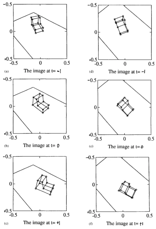
Fig. 5. Simulated image sequence a moving vehicle. (a)-(c) seen by a camera whose focal point F is located at (r, 0, q~) = (15, 45', 45'). (a) t = - 1; (b) t = 0; (c) t - + 1. Figures (d~(l) are similarly defined as that in Figs (a)~c). But the focal point of the camera is now located at (r, 0, qS) - (15, 1 5 , 4 5 i .

(8)

340 SOO-CHANG PEI and L | N - G W O LIOU

z

• i

~ !

r . ,+

"- camera

i'

o

. . .

./77_,'

" , ~ n d plane (X-Y plane) X

Fig. 6. The pose of the camera. The position of its focal point F (denoted by a vector P~) is specified by three

parametrs: r, 0, and ~D.

words, the n u m b e r of the rows of A s h o u l d be larger t h a n three a n d dim(AVA) m u s t be equal to three. If there are too m a n y missing image d a t a such t h a t the a b o v e c o n d i t i o n is not satisfied, the cost function defined in e q u a t i o n (15) is always zero a n d m a k e s n o c o n t r i b u t i o n to the total cost J any more. Similar discussion is suitable for the line features. So we have the following conclusion:

"'An image point should appear at least twice during the time interval included in the defined cost junction J. Besides, an image line Jeature should appear at least three times in the same time interval "'.

5.3. Simplification when there is no rotation

In daily experiences, the r o t a t i o n of a m o v i n g vehicle o n the r o a d is usually small. So we m a y directly set c,) and c,J. to zero a n d substitute t h e m into e q u a t i o n (26) to d e t e r m i n e the m a t r i x B. The vector a is j u s t the eigenvector c o r r e s p o n d i n g to the smallest eigenvalue of B. F r o m e q u a t i o n (26) to e q u a t i o n (30), the m o t i o n e s t i m a t i o n p r o b l e m is completely solved w i t h o u t using any iterative search.

6. EXPERIMENTAL

RESULTS

There are three goals for o u r experiments: (1) T o prove the correctness of o u r algorithm. (2) To test the r o b u s t n e s s of o u r a l g o r i t h m u n d e r different condi- tions. (3) O u r a l g o r i t h m can work well when considering a real-world image sequence. F o r a better c o n t r o l of the experiments, a simulated image sequence is a d o p t e d for the first two goals.

6.1. Experiments[or simulated image

Figures 5(a)-(c) shows a m o v i n g vehicle o n the road. T h r e e frames c a p t u r e d at t = - 1, t = 0, a n d t = + 1 are considered. Figures 5(d) (t3 shows the same m o v i n g vehicle but seen by the c a m e r a at different pose. To define the pose of the c a m e r a properly, let us see the c o n f i g u r a t i o n s h o w n in Fig. 6. The focal

(a) (b) (d)

",\

(c) (e) Fig. 7. Changing shapes of the cost function. Four cost functions are shown (a) The cost function near the true solution (has shifted to the center). (r, 0, q~)=(15, 15 °,45"). (b) Level contour: (r, 0, 4)) = (15, 15", 45+). (c) jr, 0, qS) = (15, 45', 45'). (d) (r, 0, (b) = (10, 457, 0"). (e) (r, 0, ~b) = (40, 45",0 ).

(9)

Vehicle-type motion estinaation by the fusion of image point and line features 341

center F (position vector Pc) of the camera can be represented by

P,,

= [ rsin0cos~b, rsin 0sin ~b, r c o s 0 ] . (35) The three o r t h o n o r m a l vectors, ui for i = 1 to 3, defining the pose of the camera are now set to

- P , . u 3 × ~

.

u3 = IlPcl~;

u , -

Ilu3x~lI u2 U 3 X U l , (36) Figure 5(a)-(c) considers the case when (r, 0, thl = (15, 4 5 , 4 5 ' % Figure 5(d)-(f) considers the case when

o S 0 8 7 6 5 4 3 2 1

0 i

. . .

//"

)

,1%: ~o°

- / o~,~ ° . . . .

,':

:J/~

; =S . . . 2 3

(a) _{Deviation of image position (pixel)}

(r, 0, ~b)= (15, 1 5 , 4 5 " ) . The motion parameters of the moving vehicle shown in Fig. 5 are, o~ = - 0.4, (o+ = 0 . 3 , T _ x = - 0 . 5 , T , y = - 2 . 0 , T + . x = 0 . 4 , and

T+.r

= 1.8. O n the m o v i n g vehicle, its vertices and the lines linking these vertices are used as the input image features (Np = 12 and Nt = 18). To com- pare the true solution and the estimated soluton, we define two vectors

c _ = [ ( o ,¢,~+ ]r;

d = [

T- x,T ,r, T.~.x,T+.r] 1.

{37)

[- 1 0 - - i i 9 _// " " g . . . f . . . .

,.%_-

e o ° /

7

. . . ;;7 / / 6

/'"

0=I@ "~

/

.//,

s

<

4 / ' / /1""'"

2 .//-- ~

1 L i 00 1 2

(b) Deviation of image position (pixel)

0 S 0 10 9 / Y : 4 0 g-- 7 y=20 6 5 4 .// .-/

3 ;"

/

"55

2 /:" / / / / 1 // //"

tcb

1

2

0 1 0 - ' ; ' 7 / 9 - /

Y-- 4o

,/

,,']

7

6 /'

Y'-IS,,' ~

4 ,/';

y / / ' ~

~

_.

3 " ,i'"

01 ----~-

2

3

(c) Deviation of image position (pixel) Id) Deviation of image position (pixel) Fig. 8. Error performance of the algorithm under different poses of the camera. (a) and (b) The rotation and translation errors vs. noise when varying the angle 0. (c) and (d) The rotation and translation errors

(10)

Therefore, the percentage errors of the estimated rotation and translation are separately defined as

tl~ cll

rotation error - x 100%;

Ilcil

rid -d~i

translation error - - - (38)

Ildll

The final estimation errors for Figs 5(a)-(c} and Figs 5(d} (f) are separately: ( 1 ) R o t a t i o n errors: 2.14x 10 s% and 3.45x 10 9%. (2)Translation errors: 5.82x 10 ~% and 1.05x 10 ~%. Here we assume that the true Z,~e has been given. It proves the correctness of the algorithm.

Figure 7(a) shows an example of the 2D cost function J. It is obtained by considering the same m o v i n g vehicle shown in Fig. 5. The d o m a i n of this cost function is (e)_, e~+) = [ 0.4 _+ 0.2, 0.3 _+ 0.2]. F r o m different poses of the camera, we can observe the shape change of the cost function. Figures 7(b)-(e) are

four cost functions (level contours) obtained by different positions of the camera. Figures 7(b} and (c) consider the shape change induced by different 0 (15' and 45'). Figures 7(d} and (e) consider the shape change induced by different distances r (10 and 40). We find that the cost functions corresponding to larger 0 and larger distance r will be more ill-conditioned, which may influence the robustness of our algorithm.

Figure 8(a) (d) shows the error performance under different poses of the camera. The noise-perturbed image-point positions are simulated by adding a 2D random vector (61, 62) to each vertices of the moving vehicle shown in Fig. 5. Here 6~ and 62 are random variables of normal distribution N(0, 6). 6 is the stan- dard deviation. If we assume that the total image plane (1 x 1) is uniformly divided into 512 x 512 grids, every pixel on it occupies an area of (1/5 l 2) x (1/512) square unit. Therefore, the deviation 6 = cr x (1/512) is considered as the "noise level of rr pixels ". Every point

, , ~ ~

iiiiilill[llii+l!llllllllllll!il+llUllllllll+tlHllllllllliiti!.i~l~

i U ~,.

i,,+,,,,

... , ' , ' " ,

(a)

. : !I]!.+ ' !I ],+ ]:!li:~ iltll. !il i,il f+i [i~:i : +1.

(b) ~ T t " Z i | : , *

~ i + J i + + + + , +

~ i ' ... Fi~!~I~!~+~I~I~+~I~I~t~I~T.~':~!~`~T/.~;:!~:::~;' (c)

-0.2

-0.1

+0.1

i

+0.2

_ _ ± J

- .2

0

0.2

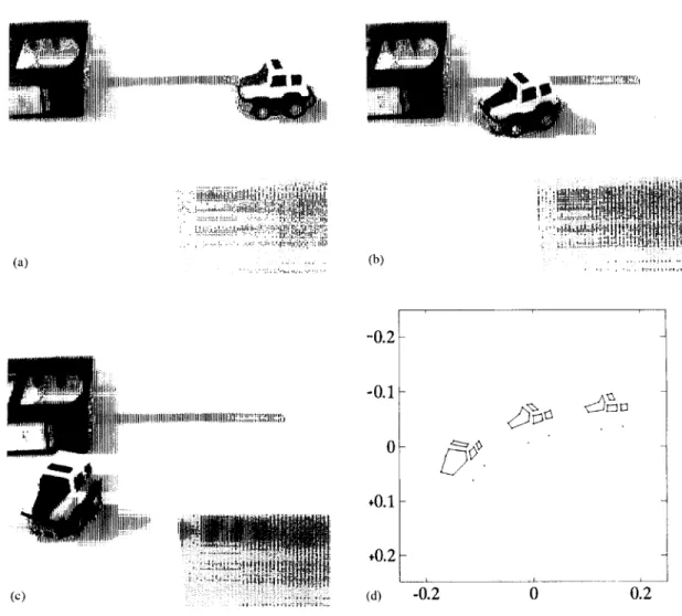
Fig. 9. Real-world image test; (a) the frame at t = 1; (b) the frame at t = 0; (c) the frame at t = + 1; (d) the extracted image points and line features (Np = 20, Nt = 18) at three time instants•

(11)

on the curves shown in Fig. 8 is the average of 40 tests. Figures (a)-(b) consider the cases when (r, 0, qS)= (15, 0, 45"). Figures 8(c) (d) consider the cases when (r, 0, qS) = (r, 4 5 , 0 ' ) . It is easy to find that the cases corresponding to larger 0 and larger distance r are more error-sensitive. The influence from the changing distance r seems stronger than that from the changing tilt angle 0.

6.2. Experiments Jot real-world image

Figures 9(a) (c) show the three frames of the testing real-world image sequence. The toy car moves from upper right to lower left. The size of the toy car is about 4.7 cm x 3.2 cm x 3.5 cm. To extract its image features (points or lines), the original image is first transformed into an "edge" image by edge detection. Both the point and line features are manually picked and traced during the three frames. To obtain a line feature, we collect all of its corresponding edge points and then determine the best-fitting line by linear regres- sion. Finally, we can trace continuously 20 points and 18 lines at three time instants. It is shown in Fig. 9(d). Following the definitions of coordinate transform described in Section 2, the pose of the camera is specified by {Re, P~}. After applying a simple camera calibration process (not shown here), we have the following parameters: aspect ratio = 1.036, focal length = 19.051 cm, viewing angle = 28', and

-0.0336 0.5066 - 0.8615"] / R,. = 0.9989 0.0099 0.0448[; 0.0312 0.8621 - 0.5057J P~ = 19.051 x -

0.0559|

cm. ! 1.3303_]

The true motion parameters of the moving toy car are directly measured as follows: [~o_, e)+] = ( - 0.3840, 0.8029) (rad), [ T - . x , T - r] = ( - 1.74, 7.87) (cm), [ Y r + . x , r + . r ] = (6.23, - 6.13) (cm). The average height Z~v~ defined in equation (30) is measured as 2.56 (cm).

Finally, the estimated results are: [v) , c~+] = ( - 0.3519,0.8306) (rad), error = 4.7640%; [ T .x,

T .y] = ( -- 1.65, 7.25)(cm), error = 7.7729%; I T + x , T+,r] = (5.69, -- 5.58) (cm), error = 8.8189%. The estimation errors may be mainly due to quantiz- ation errors, calibration errors, and position errors. But they still seem acceptable. The result could be better if a more precise camera calibration can be obtained.

7. CONCLUSIONS

In this paper, a new iterative m e t h o d is proposed for solving the problem of vehicle-type m o t i o n estimation. This m e t h o d has several advantages:

• It can handle both the point and line features as its input image data. The contributions from these image features can be fused together. All we have to do is to minimize the smallest eigenvalue of a 4 x 4 symmetry and nonnegative definitive matrix B. The dimension of searching space is very small ( = 2). • The definition of the cost function is very suitable

for parallel processing.

• Each c o m p o n e n t cost function in J has approximately the same numerical contribution to the final cost value. It is just fine to set all of the weighting factors w's defined in J to 1. Therefore, there is no serious weighting problem in our method. • Its cost function J is so well-conditioned that the

final 3D motion estimation is robust and insensitive to noise, which is proved by experiments.

• It can handle the case of missing point/line data to certain degree. Besides, a line feature has an inherent ability to handle partial occlusion.

Both the simulated and real-world images are tes- ted in this paper. Simulated experiments are mainly used to test (1) the correctness of the proposed algorithm, (2) the error performance of the proposed algorithm. The results obtained from real-world image show that our method can work well in real application.

R E F E R E N C E S

1. J. W. Roach and J. K. Aggarwal, Determine the move- ment of object from a sequence of image, IEEE Trans. Pattern Anal. Machine lntell. PAMI-2(6), 554 562 (1980).

2. H. C. Longuet-Higgins, A computer program for recon- structing a scene from two projections, Nature 293, 133 135 (1981).

3. R. Y. Tsai and Thomas S. Huang, Uniqueness and estimation of 3D motion parameters of rigid objects with curved surfaces, IEEE Trans. Pattern Anal. Machine lntell. PAMI-6(1), pp. 13 27, 1984.

4. Xinhua Zhuang, A simplification to linear two-view motion algorithms, Comput. Vision Graphics Image Pro- cess. 46, 175- 178 (1989).

5. Juyang Weng, Thomas S. Huang and Narendra Ahuja, Motion and structure from two perspective views: algorithms, error analysis, and error estimation, IEEE Trans. Pattern Anal. Machine lntell. 11(5), 451M-76 (1989). 6. Johan Philip, Estimation of 3D motion of rigid objects

from noisy observation, IEEE Trans. Pattern Anal. Ma- chine lntell. 13(1), 61 66 11991).

7. Minas E. Spetsakis and Yiannis Aloimonos, Optimal visual motion estimation: a note, IEEE Tran,s. Pattern Anal. and Machine lntell. 14(9), 959-964 (1992). 8. H. H. Chen and T. S. Huang, Maximal matching of 3D

points for multiple-object motion estimation. Pattern Reco~lnition 21(2), 75 90 (1988).

9. Vincent S. S. Hwang, Tracking feature points in time- varying images using an opportunistic selection approach, Pattern Recognition 22(3), 247-256 (1989). 10. Paul M. Griffin and Sherri L. Messimer, Feature point

tracking in time-varying images, Pattern Recoonition Lett. l l , 843 848, (1990).

11. K. Rangarajan and M. Shah, Establishing motion correspondences, CVGIP: lmaqe Understanding 54(1), 56 73 (1991).

(12)

12. B. L. Yen and T. S. Huang, "Determining 3D motion/structure of a rigid body using straight line cor- respondences, Image Sequence Proeessin,q and Dynamic

Scene Analysis, Springer, New York/Berlin, (1983).

13. A. Mitichi, S. Seida and J. K. Aggarwal, Line-based computation of structure and motion using angular in- variance, Proc. Workshop on Motion: Representation and

Analysis, IEEE Computer Soeiety, pp. 175 180, 7 9 May,

Charleston, SC (1986).

14. Yuncai Liu and Thomas S. Huang, A linear algorithm for motion estimation using straight line correspon- dences, Comput. Vision Graphies hnage Process. 44, 35 57 (1988).

15. Yuncai Liu and Thomas S. Huang, Three-dimensional motion determination from real scene images using straight line correspondences, Pattern Recognition 25(6), 617 639 (1992).

16. Minas E. Spetsakis and Yiannis Aloimonos, Structure from motion using line correspondences, Int. J. Comput.

Vision 4, 171 183 (1990).

17. Juyang Weng, Thomas S. Huang and Narendra Ahuja, Motion and structure from line correspondences: closed- form solution, uniqueness, and optimization, IEEE

Trans. on Pattern Anal. Machine lntell. 14(3), 318 335

(1992).

18. G. Medioni and R. Nevatia, Matching image using lin- ear features, IEEE Trans. Pattern Anal. Machine Intell. PAMI-6(6), 675 685 (1984).

19. J. B. Burns, A. R. Hanson and E. M. Riseman, Extracting straight lines, 1EEE Trans. Pattern Anal. Machine lntell., PAMI-8(4), 425 445 (1986).

20. F. Bergholm, Edge focusing, IEEE Trans. Pattern Anal.

Machine lntell. PAMI-9(6), 726 741 (1987).

21. Rachid Deriche and 0liver Faugeras, Tracking line seg- ments, Image Vision Comput. 8(4), 261 270 (1990). 22. T. Broida and R. Chellappa, Estimation of object motion

parameters from noisy images, IEEE Trans. Pattern

Anal. Maehine Intell. PAMI-8(1), 90~99 (1986).

23. Juyang Weng, Thomas S. Huang, and Narendra Ahuja, 3D motion estimation, understanding, and prediction from noisy image sequences, IEEE Trans. Pattern Anal.

Machine Intell. PAMI-9(3), 370-389 (1987).

24. Gwo Jyh Tseng and Arun K. Sood, Analysis of long image sequence for structure and motion estimation,

IEEE Trans. System Man and Cyhernet. 19(6),

1511 1526(1989).

25. Hormoz Shariat and Keith E. Price, Motion estimation with more than two frames, IEEE Trans. Pattern Anal.

and Machine Intell. 12(5), 417 434 (19901.

26. Ted J. Broida and Rama Chellappa, Estimating the kinematics and structure of a rigid object from a se- quence of monocular images, IEEE Trans. Pattern Anal.

Machine lntell. 13(6), 497 512 (1991).

27. Xiaoping Hu and Narendra Ahuja, Motion and structure estimation using long sequence motion models,

Image Vision Comput. 11(9), 549 569 (1993).

28. Y. F. Wang, Nitin Karandikar and J. K. Aggarwal, Analysis of video image sequences using point and line correspondences, Pattern Recognition 24(11), 1065 1084 (1991).

29. Yuncai Liu, Thomas S. Huang, and O. D. Faugeras, Determination of camera location from 2D to 3D line and point correspondences, IEEE Trans. Pattern Anal.

Machine lntell. 12(1), 28 37 (1990).

30. Mun K. Leung and T. S. Huang, Estimating 3D vehicle motion in an outdoor scene using stereo image se- quences, Int. J. lma,qing Systems Technol. 4, 81~97 (1992). 31. Yuncai Liu and Thomas S. Huang, Vehicle-type motion estimation from multi-frame images, IEEE Trans. on

Pattern Anal. Maehine lntell. 15(8), 802 808 (1993).

32. M. Spetsakis and Y. Aloimonos, A unified thoery of structure from motion, Proc. D A R P A Image Under-

standing Workshop, pp. 271 283. Pittsburgh, PA (1990).

33. M. Spetsakis, A linear algorithm for point and line based structure from motion, CVGIP: lma,qe Understandimt 56, 230 241 (1992).

About the Author LIN-GWO LIOU was born in Taiwan. He received his B.S. degree from the National

Chiao Tung University (N.C.T.U.) in Taiwan in 1989 and Ph.D. degree from the National Taiwan University in 1995, all in Electrical Engineering. Right now he is in military service His research interests include motion image analysis, methods for 3D object reconstruction, pattern recognition in image application.

About the Author SOO-CHANG PEI was born in Soo-Auo, Taiwan in 1949. He received his B.S.E.E.

from National Taiwan University in 1970 and M.S.E.E. and Ph.D. from the University of California, Santa Barbara in 1972 and 1975, respectively. He was an engineering officer in the Chinese Navy Shipyard from 1970 to 1971. From 1971 to 1975, he was a research assistant at the University of California, Santa Barbara. He was Professor and Chairman in the EE Department of Tatung Institute of Technology from 1981 to 1983. Presently, he is the Professor and Chairman of EE Department at National Taiwan University. His research interests include digital signal processing, image processing, optical information processing, and laser holography. Dr Pei is a member of the IEEE, Eta Keppa Nu and the Optical Society of America.