Spatial Autocorrelation Patterns of Understory Plant Species in a
Subtropical Rainforest at Lanjenchi, Southern Taiwan
Su-Wei Fan(1) and Chang-Fu Hsieh(1*)
1. Institute of Ecology and Evolutionary Biology, National Taiwan University. 1, Roosevelt Rd., Sec. 4, Taipei 106, Taiwan. * Corresponding author. Tel: 02-3366-2474; Fax: 02-2366-1444; Email: tnl@ntu.edu.tw
(Manuscript received 10 March 2010; accepted 18 April 2010)
ABSTRACT: Many studies described relationships between plant species and intrinsic or exogenous factors, but few quantified spatial scales of species patterns. In this study, quantitative methods were used to explore the spatial scale of understory species (including resident and transient species), in order to identify the influential factors of species distribution. Resident species (including herbaceous species, climbers and tree ferns < 1 m high) were investigated on seven transects, each 5-meter wide and 300-meter long, at Lanjenchi plot in Nanjenshan Reserve, southern Taiwan. Transient species (seedling of canopy, subcanopy and shrub species < 1 cm diameter at breast height) were censused in three of the seven transects. The herb coverage and seedling abundance were calculated for each 5 × 5 m quadrat along the transects, and Moran’s I and Galiano’s new local variance (NLV) indices were then used to identify the spatial scale of autocorrelation for each species. Patterns of species abundance of understory layer varied among species at fine scale within 50 meters. Resident species showed a higher proportion of significant autocorrelation than the transient species. Species with large size or prolonged fronds or stems tended to show larger scales in autocorrelation. However, dispersal syndromes and fruit types did not relate to any species’ spatial patterns. Several species showed a significant autocorrelation at a 180-meter class which happened to correspond to the local replicates of topographical features in hilltops. The spatial patterns of understory species at Lanjenchi plot are mainly influenced by species’ intrinsic traits and topographical characteristics.
KEY WORDS: Spatial autocorrelation, Moran’s I, new local variance (NLV), herbaceous species, seedlings and functional traits.
INTRODUCTION
Understanding spatial patterns provides vital clues to the influential factors of species distribution and helps to generate hypotheses about their relationships (Ford and Renshaw, 1984). Therefore, simultaneously quantifying spatial scales for both of species’ intrinsic and external factors can provide both biological and environmental information in controlling factors (Dale, 2000). Many studies revealed that the variability of environmental factors can directly influence the spatial pattern of plants. For example, Pool (1914) was the first scientist who recognized the association between topography and species in a Nebraska Sandhills; later, the distribution of grass species were proved to be controlled by spatial distribution of available water along a topographic gradient in the same area (Barnes and Harrison, 1982). Spatial association patterns between plants and topography in tropical areas are also shown at various scales, including local (He et al., 1997; Condit et al., 2000), meso- (Clark et al., 1998) and regional scales (Newbery et al., 1986; Tuomisto and Ruokolainen, 1994). Those spatial scales and distribution patterns may reflect niche requirements of a species and availability of environmental resources (Dale, 2000).
The forest understory (including resident species and transient species) is an important component of biodiversity with both intrinsic and functional values
(Whitney and Foster, 1988; Poulsen and Balsley, 1991; Scheiner and Istock, 1994; Tchouto et al., 2006). Resident species, such as herbs and small shrubs, are those with life-history characteristics that confine them to above-ground height of ca. 1-1.5 meter (Gilliam and Roberts, 2003). Transient species comprise plants whose existence in understory layer is temporary because they have potential to develop and emerge into higher strata (e.g., subscanopy and canopy strata) (Gilliam and Roberts, 2003). The stratum of forest vegetation containing resident species often called the herbaceous layer. The herbaceous layer can serve as a "filter" for future canopy trees (Royo and Carson, 2008), and provides both food and habitat for a wide array of animal species (Martin et al., 1951; Pough et al., 1987). However, the studies of understory vegetation were relatively few comparing to overstory investigation (Hart and Chen, 2006). Here we examine the spatial patterns of understory vegetation in a subtropical forest with the intention for revealing determining factors of this stratum.
The emergence of understory species is influenced by both extrinsic and intrinsic processes that occur over small areas. Abundance pattern of an understory species may reflect on the spatial characteristic of an external factor such as micro-topography (Bratton, 1976; Beatty, 1984). For example, in neotropical forests, understory fern and palm cover appear positive relatedness to soil fertility and moisture (Wright, 1992) and seedling density was
negatively correlated with palm cover (Harms et al., 2004). Intrinsic traits of species such as dispersal ability and reproduction traits can also influence species distribution patterns. For example, wind-dispersal syndromes are fairly evenly distributed at all elevations and distance from river banks, comparing with plants dispersed by animals (Drezner et al., 2001; Miller et al., 2002). Plant with vigorous vegetative growth and large individual size are autocorrelated in a broader scale than species without vegetative propagules and show a patched distribution pattern in local scale (Verburg et al., 1996). Relationships between the spatial pattern and intrinsic traits of plants or between plant and spatial heterogeneity can be detected using quantitative methods. For example, Kershaw (1964) found that in Eriophorum angustifolium and Trifolium repens, the first three scales of distribution patterns are related to their length of branch growth and to their stolon or rhizome system.
Nanjenshan forests, on the southern tip of Taiwan, harbor some of best examples of lowland forests in subtropical region. The overstory vegetation of Nanjenshan forests were attracted much attention and well-investigated (Chao et al., in press) because of their mixture of holarctic and tropical plant elements (Li and Keng, 1950; Huang et al., 1980). However, the study of understory vegetation is still limited. In this study, quantitative methods (i.e., autocorrelations and new local variance) were used to explore the patterns of species distribution and species abundance in understory layer. We ask the following questions (1) what are the autocorrelation scales of understory species distributions, and (2) what are the major determining factors for the autocorrelation patterns of understory species. Specifically, we ask that if there are any intrinsic traits of understory species (e.g., reproduction traits, individual size, and life forms) or exogenous factor (i.e., topography) showing correlations with the spatial scales of understory species.
MATERIALS AND METHODS
Study site
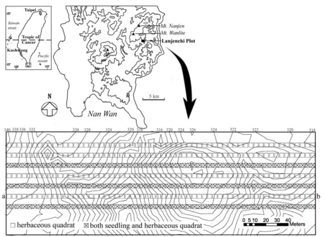
Lanjenchi Forest Dynamics Plot (22°3’N, 120°51’E), in the Nanjenshan Reserve of the Kenting National Park is located on the eastern slope of the Central Mountain Range near the coast of the Pacific Ocean in southern Taiwan (Fig. 1). The climate is coastal and tropical with a mean annual temperature of 22.3°C (recorded from 1994 to 1998) and monthly mean temperature ranging 18°C in January to 26.1°C in July. The average annual precipitation is 3,793 mm and 72 percent of it occurred between June and October mainly by typhoons. The forest in the Nanjenshan reserve was
classified as a monsoon forest (Su and Su, 1988). Although the elevation is low (about 300 to 350 m above sea level), forests here were classified as a Machilus-Castanopsis forest by the vegetation classification system of Taiwan (Su, 1984) and the oerstory is constituted of evergreen oak-laurel species, due to the influence of monsoon (Liu and Liu, 1977). The 3 ha Lanjenchi Forest Dynamics Plot (100 m by 300 m) was established in 1989 (Fig. 1). The plot has moderate relief with slopes mostly between 10 and 30% and elevation ranging from 300 to 350 m above sea level. The plot is crossed by a small north-south oriented creek and separated the plot into hills (Fig. 1). The exposed geological strata consist of interbedded sandstones and shales of Miocene age (Chen et al., 1997).
Field sampling
Field work for understory vegetation was carried out from July to October in 1991. For resident species (i.e., herbaceous species, including climbers and tree ferns < 1 m in height), 420 contiguous quadrats, each five meter by five meter, on seven transects in the Lanjenchi Forest Dynamics Plot were established (Fig. 1), and the resident plants sampled within each quadrat were identified and recorded. The coverage of each species was measured by line intercept method along two transect lines within each quadrat, which were set one meter from the northern and from the southern borders of each quadrat. Among the seven transects, three of them were selected to census transient species (i.e., seedlings of canopy, subcanopy and large shrub species < 1 cm diameter at breast height). A total of 180 contiguous quadrats on three transects were established (Fig. 1) and all seedlings within each quadrat were identified and recorded. Nomenclature, life forms, individual heights, dispersal syndromes and vegetative tissues of understory species followed the definition in the Flora of Taiwan (Huang, 1993-2000).
Analysis
Coverage for each herbaceous species in each quadrat was calculated as the sum of the intercept lengths divided by the total sampled length (10 m in each quadrat). Abundance of seedling species in each quadrat was evaluated as the number of individuals within the sample area. The herb coverage and seedling abundance were used to quantify spatial scale for each species. Two indices, Moran’s I (1950) and Galiano’s new local variance (Galiano, 1982) were computed in spatial analysis.
Moran’s I, a spatial autocorrelation coefficient, estimates the similarity of sampled values within a certain distance class. The Moran’s I is calculated as:
Fig. 1. Locations of the study site, Lanjenchi Plot in Nanjenshan Reserve of the southernmost part of Taiwan (22°3’N and 120°51’E) and contiguous quadrats for sampling seedling abundance and herbaceous coverage. (The second last transect (a-b) in the study plot was used for constructing the correlogram shown in Fig. 2).
i h for y y y y y y w d I i n i n i h hi n i n h w ≠ − Σ − − Σ Σ = = = = 2 1 1 1 1 1 ) ( ) )( ( ) ( … (1)
The yh and yi are the values of the observed variables at
quadrats h and i; d is a distance class and n is the number of sampled quadrats. The weights whi = 1 when sites h
and i at distance d and whi=0 otherwise; w is the number
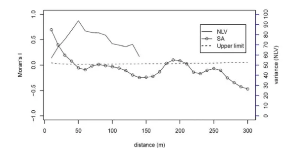
of quadrat pairs at d distance. For the autocorrelation pattern, in the beginning the similarity values (in Moran’s I) of samples decreases with the increase of distances, and becomes level and not significantly different from 0 when the autocorrelation cannot be detected. However, the value of Moran’s I could be significantly larger than 0 again if there are some replicates of environmental conditions. Under these circumstances, the scale of autocorrelation pattern is defined as the distance at which similarity values (in Moran’s I) becomes level and not significantly different from 0. A correlogram is a graph in which autocorrelation values (Moran’s I) are plotted against distance classes (Legendre and Legendre, 1998). For example, Fig. 2 is a correlogram of quadrat slope along the second last transect (a-b) in the study plot (Fig. 1)
and the similarities of topographical slopes between sampled quadrats decline with the increasing distance in the Lanjenchi plot. The scale of spatial pattern for the topographical index (slope) was ca. 50 meters (Fig. 2). Randomization test of significance was used for each individual autocorrelation coefficient and the 95% upper limits against distance classes can be plotted as dashed line on Fig. 2. The autocorrelation values above dashed line mean that the samples at this distance were significantly positively correlated. For example, the spatial autocorrelation pattern became significant again in ca. 180 meters distance class (Fig. 2), which reflected the distance between the two replicates of hilltops within the study plot. Galiano ‘s new local variance (NLV) is a quadrat variance method for detecting the size of distributed patches rather than as a method for estimating scales of spatial pattern (Dale, 2000). However, it can only be used in contiguous sampling. The variance is calculated as:
−
Σ
−
Σ
Σ
=
+ − + = − + = − = 11 2 1 2 2 1(
)
)
(
j b i b i j j b i j b n i Nb
y
y
V
)
2
(
2
/
)
(
Σ
ij+=bi+1y
j−
Σ
ij+=2ib+b+1y
j 2b
n
−
b
…(2)Fig. 2. Construction of a correlogram and a variogram, using Moran’s I (SA) and new local variance (NLV), respectively. The correlogram was generated using slopes values of 420 herbaceous quadrats and the variogarm was generated using contiguous quadarts of transect a-b (indicated in Fig. 1). The upper limits of Moran’s I estimated by randomization method were also plotted in dahed lines.
The yi is the value of the observed variable at quadrat i; n
is the number of quadrats in a transect. NLV examines the average of squared differences between duos of adjacent blocks of size b. The peak in a variogram of NLV values (as a function of distance) is interpreted as the average patch size of the pattern. For example, Fig. 2 showed that in Nanjenshan, the average patch size of slope changed in 50 meters, which is similar to the results by the Moran’s I correlogram.
In this study we examined the spatial scale and patch size for understory species were estimated by Moran’s I and NLV respectively. Species was strongly aggregated and patchily distributed in Lanjenchi plot, thus there would be some absent data in part of the sampled quadrats. When using data with absent values, all the species would be significant in autocorrelation calculations. Therefore, those quadrats with an absent (zero) were eliminated from computing Moran’s I in order to emphasize the correlation within a finer environmental scale for species in Lanjenchi plot. Because NLV uses only contiguous sampling, the absent value cannot be eliminated. Coverage or abundance data of resident and transient species scattered in seven and three transects respectively; there were seven replicates of NLV calculation for resident species and three replicates for seedling species. Patch size was defined as the minimal distance of spatial scale class with maximal variance among replicates.
In terms of external (environmental) factors, we compared the results of Moran’s I spatial scale for available data between resident species and transient species. We assume that if there is a similar proportion of species showed significant spatial scale for both resident species and transient species, this would indicate that
there are similar external (environmental) factors can influence both types of species. Otherwise, the two types of species were controlled by different external factors. In terms of intrinsic (biological) factors, we compared the results of Moran’s I spatial scale for available data within resident species for their vegetative growth types, including with and without rhizomes, and with prolonged tissue (fronds or stems). We assume that if with rhizome or prolonged tissues is contributing factor for spatial patterns, then the proportion of species has significant autocorrelation scales would be in broader distances (i.e., larger spatial scale) than species without rhizomes or prolonged tissue, due to with rhizomes or with prolonged tissue can help extend the distribution range of species (Verburg et al., 1996). As for the intrinsic factors (sexual reproductive traits), we compared the results of Moran’s I spatial scale for their life forms (i.e., “canopy” or “subcanopy and shrub” in transient species), dispersal syndromes (wind-dispersed or not), and fruit types (i.e., berry, capsule, drupe and fruits). We assume that a canopy life form, a “wind-dispersed” species, or berry fruit type would have a broader spatial scale than other species, due to a larger individual size (Verburg et al., 1996; Kuuluvainen et al., 1998) or longer-distance dispersal of winds and birds (Drezner et al., 2001; Miller et al., 2002).
RESULTS
A total of 150 understory species, consisting of 45 resident herbaceous species and 60 transient woody species, could be used in spatial analysis because of sufficient presence data in more than 30 quadrats. The results showed larger phase sizes (in NLV) than spatial
Fig. 3. Numbers of resident and transient species showing significant autocorrelations in each distance spatial scale class.
scales (in Moran’s I) of most species especially in trnsient species. However, separating resident and transient species, the estimated spatial scale and phase size showed a roughly consistent trend among species (Appendix).
Values of spatial autocorrelation generally decreased with distance for most species. Also, with the increase of spatial scale, there was a decline of species number with significant autocorrelation results (Fig. 3). The peaks on variogram of NLV values against distance were located at various distance classes among species. Therefore, understory species had varied spatial scales and patch sizes (Appendix).
Most species (> 98% of species) showed patch size and spatial scale at distance class less than 50 meters by Galiano’s NLV and Moran’s I. Comparing spatial patterns between resident and transient species at fine scale within 50 meters, larger number of resident species showed significant autocorrelation in various distance classes which indicated that resident species generally had large spatial scale than transient species (Fig. 3). There was a peak at 180 meter spatial scale on Fig. 3, due to several species showed significant autocorrelations at broader scales. Therefore, in Lenjenchi plot, the spatial pattern of species might be influenced by both fine- and broad-scale factors.
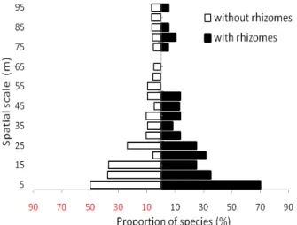
In terms of vegetative growth types, all resident species were perennial and more than half resident species (53 %) were with rhizomes in Lanjenchi plot (Appendix). A high proportion of significant autocorrelation among rhizomed species were showed only at five meter spatial scale, but were not differedat other broader spatial scale (Fig. 4). This indicated that the possession of rhizomes did not significantly contribute to the spatial scale of species. However, seven of ten species with prolonged fronds or stems in
Fig. 4. Proportions of species (with and without rhizomes) showing significant autocorrelations in each distance spatial scale class.
vegetative growth types (e.g., Dicranopteris linearis, Liriope spicata, Schizostachyum diffusum) tended to show significant autocorrelation at more than five meter distance classes (Table 1). The spatial scale of resident species correlated with their individual height (Pearson correlation: 0.473, p < 0.05); this showed a relationship between spatial scale and individual size.
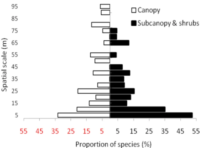
In terms of life form, seedlings of shrub and subcanopy species showed high proportions of significant autocorrelation at fine scales within 50 meters (Fig. 5), which is not as expected. Comparing spatial pattern among different dispersal syndromes, we did not find larger scale of significant autocorrelation for wind-dispersed species than for species with other dispersal syndromes, which is also not as expected (Table 1). Species among different fruit types (i.e., berry, capsule, drupe and nut fruits) did not showed a particular pattern of autocorrelations, but species with berries showed a large number of species with significant autocorrelation at ten meter spatial scale (Table 1).
DISCUSSION
Species had different spatial autocorrelation scales ranging from five to 40 meters. This information of spatial scales among species can help us to understand the crucial factors contributing to species occurrences and also a basic criterion of sampling design. Spatial autocorrelation may also causes misinterpretation in statistical tests than the data can actually justify because the number of truly independent observations may be less than what were used in the tests (Legendre, 1993; Thomson et al., 1996). For example, spatial scale of herbaceous species (e.g., Schizostachyum diffusum) can be larger than 40 meters. This indicates a unique prolonged growth pattern for this climbing species. Moreover, when examining the
Fig. 5. Proportions of species (”canopy” or “subcanopy and shrubs”) showing significant autocorrelations in each distance spatial scale class.
relationship between abundance of Schizostachyum diffusum and the density of woody seedling under a herbaceous layer using a quadrat-based method, each quadrat should be at least apart from each other for more than 40 meters. The sample quadrats in a smaller spatial scale than autocorrelation spatial scale would result in pseudo-replication and dependent of data.
Understory species had different spatial scales between resident and transient species; this showed that characteristic of species may affect their spatial scales. Resident species with large individual size are easy to form a larger size of distribution patch than those with small individual size in spatial patterns (Verburg et al., 1996; Miller et al., 2002). Therefore, in Nanjenshan forest, a single herb (e.g., tree ferns and palms) with
relatively big individual size (large individual height) might occupy a large area over several quadrats, causing spatial autocorrelation between neighboring quadrats. The well adaptation to changes of environmental conditions of understory species may increase their abundance and form a large patch size in spatial patterns (Einsmann et al., 1999). Herbaceous species was considered to own a quick development of root systems and could quickly reflect on environmental fluctuations; they also showed a greater scale of response to external conditions (Einsmann et al., 1999). Therefor, several herbaceous species (e.g., Pleocnemia rufinervis, carex makinoensis and Alpinia oblongifolia) showed large spatial scale in our results. Shrub and subcanopy seedlings (e.g. Psychotria rubra, Lasianthus spp.) rather than most canopy species also showed a large spatial scale in our study. The seedlings of shrubs defined in our study (1 meter high) might be mature enough to be in adult phase rather than in seedling phase and well adapted to understory condition, showing a large spatial scale. Except for size-related spatial pattern, vegetative growth of species also influenced the spatial pattern (Kershaw, 1964; Dale and Macisaac, 1989). For example, herbs with prolonged stems and fronds tended to have large spatial scales (Table 1) and patch sizes (Appendix) of distribution patterns. Rhizome is one of the common vegetative organs of perennial herbs (Buell and Wilbur, 1948; Cain, 1950). Herbaceous species in Lanjenchi plot were all perennial and half of them with rhizomes. However, the existence of rhizomes in a plant did not always indicate large spatial scale (11 of 24 species with rhizomes showing small spatial scale within five meters). Comparing to prolonging stems, rhizomes may express different functions such as storage and generation of Table. 1. Summary of spatial scales (minimal distance with non-significant autocorrelation by Moran’s I) among different life forms, vegetative growth types for resident species, dispersal syndromes and dispersed fruit types (excluded the wind-dispersed diaspore). Spatial scale (m) Number of species 5 10 15 20 25 30 35 40 Life form Canopy tree (N=34) 28 3 3 0 0 0 0 0 Subcanopy tree (N=11) 7 3 1 0 0 0 0 0 Shrub (N=15) 10 2 1 1 0 0 1 0 Tree-like fern (N= 1) 0 0 0 1 0 0 0 0 Herb (N=36) 21 8 2 2 1 1 1 0 Climber (N=8) 3 2 0 1 0 1 0 1
Vegetative growth types
With rhizomes (N=24) 11 7 2 0 1 1 1 1
With prolonged tissue (N=10) 3 2 0 3 0 1 0 1
Dispersal syndrome
Wind-dispersed (N=27) 17 6 2 2 0 0 0 0
Others (N=78) 52 12 5 3 1 2 2 1
Dispersed fruit types
Berry (N=22) 13 6 1 1 0 0 1 0
Capsule (N=11) 8 2 1 0 0 0 0 0
Drupe (N=26) 18 2 3 1 0 1 1 0
Nut (N= 6) 6 0 0 0 0 0 0 0
ramets as substitutes for old ones. Therefore, a dormant rhizome with function of storage may not expand population size; small vegetative growth organs may only create small patches barely to detect in spatial analysis. As the quadrat size of our study was 5 by 5 meter, we cannot detect any spatial autocorrelation smaller than a five-meter scale.
The sexual reproduction traits of species (i.e., dispersal syndromes and fruit types for all understory species) did not relate to spatial scale. Diaspores with different dispersal syndromes and fruit types might show different dispersal distance, for example, wind-dispersed type > aminal-dispersed type and ingested type (berry) > adhesive type (others) (Drezner et al., 2001; Miller et al., 2002). Dispersal ability can influence the spatial scale (Miller et al., 2002). However, the relationship between spatial scale and dispersal abilities could not be revealed among species in our results. The dispersal limitation among different fruit types might exist in a broad scale larger than 300 meters. As for the experimental design, the longest distance interval between quadrats was 300 meters, it not allowed to detect spatial autocorrelation large than 300 meters.
Spatial patterns of species in Lanjenchi were related to life traits at fine scale within 50 meters and were simultaneously affected by topographical position in broad scale. Previous studies pointed out that vegetation types and plant distributions in Lanjenchi plot were strongly affected by the interaction of topography and northeast monsoon (Chen et al., 1997; Sun et al., 1998; Chao et al., 2007). Hence the vegetation varied according to topographical positions and was classified into windward and leeward types. Most of the species could be classified as windward-, leeward- and widely distributed types (Cheng, 1992; Sun, 1993; Chao et al., in press). These all showed the different response of plant species to exogenous factors. Two hilltops ca. 180 meters apart in the study plot provided similar micro-habitats and several herbaceous species corresponded to this broader scale replication of habitats, especially for the resident species (Fig. 3).
In conclusion, our study indicated that the spatial patterns of species were influenced by both intrinsic (life form) and exogenous factors (topographic features). The vegetative growth patterns (prolonged tissue) for resident species and were much important than the sexual reproductive traits (dispersal syndromes) for a local spatial scales within 50 meters. The topographical spatial characteristic was also one of the major exogenous factors to influence spatial patterns for both resident and transient understory species at Lanjenchi Plot, southern Taiwan.
ACKNOWLEDGEMENTS
We greatly appreciate the staff of Kenting National Park for their support and permission to use the workstation at Nanjenshan Reverse. We are also grateful to all of the volunteers from many colleges for their participation in the field works. Financial support was provided by the Kenting National Park of the Republic of China.
LITERATURE CITED
Barnes, P. W. and A. T. Harrison. 1982. Species distribution
and community organization in a Nebraska Sandhills mixed prairie as influenced by plant/soil-water relationships. Oecologia 52: 192-201.
Beatty, S. W. 1984. Influence of microtopography and canopy
species on spatial patterns of forest understory plants. Ecology 65: 1406-1419.
Bratton, S. P. 1976. Resource division in an understory herb
community - responses to temporal and microtopographic gradients. Am. Nat. 110: 679-693.
Buell, M. F. and R. L. Wilbur. 1948. Life-form spectra of the
hardwood forests of the Itasca Park region, Minnesota. Ecology 29: 352-359.
Cain, S. A. 1950. Life-forms and phytoclimate. Bot. Rev. 16:
1-32.
Chao, W.-C., K.-J. Chao, G.-Z. M. Song and C.-F. Hsieh.
2007. Species composition and structure of the lowland subtropical rainforest at lanjenchi, southern Taiwan. Taiwania 52: 253-269.
Chao, W.-C., G.-Z. M. Song, K.-J. Chao, C.-C. Liao, S.-W. Fan, S.-H. Wu, T.-H. Hsieh, I.-F. Sun, Y.-L. Kuo and C.-F. Hsieh. in press. Lowland rainforests in southern
Taiwan and Lanyu, at the northern border of Paleotropics and under the influence of monsoon wind. Plant Ecol. in press.
Chen, Z.-S., C.-F. Hsieh, F.-Y. Jiang, T.-H. Hsieh and I.-F. Sun. 1997. Relationship of soil properties to topographphy
and vegetation in a subtropical rain forest in southern Taiwan. Plant Ecol. 132: 229-241.
Cheng, Y.-B. 1992. The understory of the subtropical rain forest
in Nanjenshan area [dissertation]. National Taiwan University, Taipei, Taiwan. 72pp.
Clark, D. B., D. A. Clark and J. M. Read. 1998. Edaphic
variation and the mesoscale distribution of tree species in a neotropical rain forest. J. Ecol. 86: 101-112.
Condit, R., P. S. Ashton, P. Baker, S. Bunyavejchewin, S. Gunatilleke, N. Gunatilleke, S. P. Hubbell, R. B. Foster, A. Itoh, J. V. LaFrankie, H. S. Lee, E. Losos, N. Manokaran, R. Sukumar and T. Yamakura. 2000. Spatial
patterns in the distribution of tropical tree species. Science
288: 1414-1418.
Dale, M. R. T. 2000. Spatial pattern analysis in plant ecology.
Cambridge University Press, Cambridge, England, UK. 326pp.
Dale, M. R. T. and D. A. Macisaac. 1989. New methods for the
analysis of spatial pattern in vegetation. J. Ecol. 77: 78-91.
Drezner, T. D., P. L. Fall and J. C. Stromberg. 2001. Plant
distribution and dispersal mechanisms at the Hassayampa River Preserve, Arizona, USA. Glob. Ecol. Biogeogr. 10: 205-217.
Einsmann, J. C., R. H. Jones, M. Pu and R. J. Mitchell. 1999.
contrasting life forms. J. Ecol. 87: 609-619.
Ford, E. D. and E. Renshaw. 1984. The interpretation of
process from pattern using two-dimensional spectral-analysis - modeling single species patterns in vegetation. Vegetatio. 56: 113-123.
Galiano, E. F. 1982. Detection and measurement of
one-species patterns in grasslands. Acta. Oecol. 3: 269-278.
Gilliam, F. S. and M. R. Roberts. 2003. Conceptual
framework for studies of the herbaceous layer. In: Gilliam, F. S. and M. R. Roberts (eds.), The herbaceous layer in forest of eastern north America, Oxford university press, New York, USA. pp. 3-11.
Harms, K. E., J. S. Powers and R. A. Montgomery. 2004.
Variation in small sapling density, understory cover, and resource availability in four Neotropical forests. Biotropica. 36: 40-51.
Hart, S. A. and H. Y. H. Chen. 2006. Understory vegetation
dynamics of North American boreal forests. Crit. Rev. Plant Sci. 25: 381-397.
He, F., P. Legendre and J. V. Lafrankie. 1997. Distribution
patterns of tree species in a Malaysian tropical rain forest. J. Veg. Sci. 8: 105-114.
Huang, T.-C., Y.-C. Kuo, Y.-C. Chen and T.-L. Huang.
1980. The vegetation survey of Kenting National Park., Kenting park publication, National Park Service, Taiwan.
Huang, T. C. (ed.). 1993-2000. Flora of Taiwan. Department
of Botany, National Taiwan University, Taipei, Taiwan.
Kershaw, K. A. 1964. Quantitative and dynamic ecology.
Edward Arnold, London, UK. 183pp.
Kuuluvainen, T., E. Jarvinen, T. J. Hokkanen, S. Rouvinen and K. Heikkinen. 1998. Structural heterogeneity and
spatial autocorrelation in a natural mature Pinus sylvestris dominated forest. Ecography 21: 159-174.
Legendre, P. 1993. Spatial autocorrelation - trouble or new
paradigm. Ecology 74: 1659-1673.
Legendre, P. and L. Legendre. 1998. Numerical ecology.
Elsevier press, Amsterdam, the Netherlands, New York, NY, USA. 853 pp.
Li, H. L. and H. Keng. 1950. Phytogeographical affinities of
southern Taiwan. Taiwania 1: 103-122.
Liu, T.-S. and J.-Y. Liu. 1977. Synecological studies on the
natural forest of Taiwan III : Studies on the vegetation and Flora of Nanjenshan area on Hengchun Peninsula. Ann. Taiwan Mus. 20: 51-149.
Martin, A. C., H. S. Zim and A. L. Nelson. 1951. American
wildlife & plants : a guide to wildlife food habits; the use of trees, shrubs, weeds, and herbs by birds and mammals of the United States McGraw-Hill, New York, USA. 500pp.
Miller, T. F., D. J. Mladenoff and M. K. Clayton. 2002.
Old-growth northern hardwood forests: Spatial autocorrelation and patterns of understory vegetation. Ecol. Monogr. 72: 487-503.
Moran, P. A. P. 1950. Notes on continuous stochastic
phenomena. Biometrika. 37: 17-23.
Newbery, D. M., E. Renshaw and E. F. Brunig. 1986. Spatial
pattern of trees in Kerangas Forest, Sarawak. Vegetatio. 65: 77-89.
Pool, R. J. 1914. A study of the vegetation of the sandhills of
Nebraska. Minn Bot Stud 4: 189-312.
Pough, F. H., E. M. Smith, D. H. Rhodes and A. Collazo.
1987. The Abundance of Salamanders in Forest Stands with Different Histories of Disturbance. For Ecol Manage 20: 1-9.
Poulsen, A. D. and H. Balsley. 1991. Abundance and cover of
ground herbs in an Amazonian rain-forest. J Veg Sci 2: 315-322.
Royo, A. A. and W. P. Carson. 2008. Direct and indirect effects
of a dense understory on tree seedling recruitment in temperate forests: habitat-mediated predation versus competition. Can. J. For. Res. 38: 1634-1645.
Scheiner, S. M. and C. A. Istock. 1994. Species enrichment in a
transitional landscape, northern lower Michigan. Can J. Bot.
72: 217-226.
Su, H.-J. 1984. Studies on the climate and vegetation types of the
Natural forests in Taiwan (II) Alitudinal vegetation zones in relation to temperature gradient. Q. J. Chi. For. 17: 57-73.
Su, H.-J. and C.-Y. Su. 1988. Multivariate analysis on the forest
vegetation of Kenting National Park, Southern Taiwan. Q. J. Chi. For. 21: 17-32.
Sun, I.-F. 1993. The species composition and Forest structure of
a subtropical rain forest at southern Taiwan [dissertation] University of California at Berkeley. 205pp.
Sun, I.-F., C.-F. Hsieh and S. P. Hubbell. 1998. The structure
and species composition of a subtropical monsoon forest in southern Taiwan on a steep wind-stress gradient In: Dallmeier, F. and J. A. Comiskey (eds.), Forest Diversity Research, monitoring and modeling: conceptial background and old word case studies, Parthenon Publishing Co., Paris, France. pp. 565-635.
Tchouto, M. G. P., W. F. De Boer, J. De Wilde and L. J. G. Van der Maesen. 2006. Diversity patterns in the flora of the
Campo-Ma'an rain forest, Cameroon: do tree species tell it all? Biodivers. Conserv. 15: 1353-1374.
Thomson, J. D., G. Weiblen, B. A. Thomson, S. Alfaro and P. Legendre. 1996. Untangling multiple factors in spatial
distributions: Lilies, gophers, and rocks. Ecology 77: 1698-1715.
Tuomisto, H. and K. Ruokolainen. 1994. Distribution of
Pteridophyta and Melastomataceae along an edaphic gradient in an Amazonian rain-forest. J. Veg. Sci. 5: 25-34.
Verburg, R. W., R. Kwant and M. J. A. Werger. 1996. The
effect of plant size on vegetative reproduction in a pseudo-annual. Vegetatio. 125: 185-192.
Whitney, G. G. and D. R. Foster. 1988. Overstorey
composition and age as determinants of the understorey flora of woods of central New England. J. Ecol. 76: 867-876.
Wright, S. J. 1992. Seasonal drought, soil fertility and the
species density of tropical forest plant communities. Trends. Ecol. Evol. 7: 260-263.
Appendix. Summary of biological characteristics of 105 understory species of Lenjenchi plot in Nanjenshan Reserve, Taiwan. N = the number of quadrats containing this species; SA= the minimal distance class showing non-significant spatial autocorrelation (Moran’s I) within 50-meter scale; NLV= the distance class at which large variance occurred. IV= importance values of species, calculated as percent coverage for resident species and relative basal area of large trees ( ≥ 1 cm DBH) for transient species. Scientific name N Max. Cover (%) Spatial scale (m) IV (%) Ind. height (m)
Life form diaspore
size (cm3)diaspore vegetative growth
SA NLV
Understory resident species
Pteridophyte
Aspidiaceae
Hemigramma decurrens 62 25 5 5 0.66 0.3 herb <0.001 wind-dispersed spore rhizomes
Pleocnemia rufinervis 173 62 15 25 4.99 0.5 herb <0.001 wind-dispersed spore rhizomes
Athyriaceae
Diplazium dilatatum 166 55 10 10 3.13 0.4 herb <0.001 wind-dispersed spore rhizomes
Diplazium donianum 208 88 10 10 8.61 0.4 herb <0.001 wind-dispersed spore rhizomes
Blechnaceae
Blechnum orientale 39 28 5 5 0.63 0.8 herb <0.001 wind-dispersed spore underground
storage tissue Cyatheaceae
Alsophila podophylla 239 91.5 20 20 11.66 1.5 tree-like <0.001 wind-dispersed spore
Dryopteridaceae
Dryopteris sordidipes 153 35 5 5 0.94 0.3 herb <0.001 wind-dispersed spore rhizomes
Gleicheniaceae
Dicranopteris linearis. 75 100 20 5 4.14 0.5 herb <0.001 wind-dispersed spore prolonged
frond Hymenophyllaceae
Cephalomanes laciniatum 31 4 5 5 0.05 0.2 herb <0.001 wind-dispersed spore rhizomes
Lindsaeaceae
Lindsaea merrillii ssp.
yaeyamensis 133 12 10 5 0.50 0.2 herb <0.001 wind-dispersed spore rhizomes
Lindsaea orbiculata var.
deltoidea 206 14 10 5 0.80 0.5 herb <0.001 wind-dispersed spore rhizomes
Tapeinidium pinnatum 106 41.5 15 10 1.27 0.3 herb <0.001 wind-dispersed spore rhizomes
Pteridaceae
Pteris grevilleana 34 5 5 5 0.05 0.5 herb <0.001 wind-dispersed spore rhizomes
Pteris plumbea 33 4 5 5 0.04 0.3 herb <0.001 wind-dispersed spore rhizomes
Selaginellaceae
Selaginella doederleinii 58 9 10 5 0.10 0.15 herb <0.001 wind-dispersed spore rhizomes
Thelypteridaceae
Pronephrium cuspidatum. 45 16 5 5 0.42 0.3 herb <0.001 wind-dispersed spore rhizomes
Pronephrium triphyllum 65 20 5 5 0.57 0.2 herb <0.001 wind-dispersed spore rhizomes
Dicotyledon
Acanthaceae
Codonacanthus pauciflorus 39 0.2 5 5 0.01 0.15 herb 0.002 capsule
Asteraceae
Farfugium japonicum var.
formosanum 99 10 10 5 0.26 0.3 herb 0.085
wind-dispersed
achenes rhizomes
Piperaceae
Piper kawakamii 197 9 5 5 0.20 0.15 climber 0.019 berry prolonged
stem Rubiaceae
Psychotria serpens 319 19 10 5 0.70 0.1 climber 0.206 drupe prolonged
stem Urticaceae
Elatostema lineolatum var.
major. 35 38.5 5 5 0.81 0.4 herb <0.001
wind-dispersed achenes
Monocotyledon
Araceae
Pothos chinensis 115 7.5 5 5 0.17 0.15 climber 0.520 animal-dispersed berry
Arecaceae
Calamus formosanus 266 78 20 10 10.79 1.2 climber 0.520 fruit prolonged
Appendix. Continued. Scientific name N Max. Cover (%) Spatial scale (m) IV (%) Ind. height (m)
Life form diaspore size (cm3)diaspore vegetative growth
SA NLV
Calamus quiquesetinervius 252 60 10 10 6.79 1 climber 3.062 fruit prolonged
stem Cyperaceae
Carex makinoensis 217 100 30 15 13.50 0.4 herb 0.002 achenes rhizomes
Scleria terrestris 164 18 5 5 0.65 0.8 herb 0.006 achenes rhizomes
Dioscoreaceae
Dioscorea japonica var.
pseudojaponica 86 5 5 5 0.03 0.2 climber
3.033
capsule prolonged
stem Liliaceae
Aspidistra elatior var.
attenuata 48 46 10 5 0.71 0.5 herb
0.520
berry rhizomes
Dianella ensifolia 83 19 5 5 0.51 0.5 herb 0.520 berry rhizomes
Liriope spicata 327 44.5 20 10 3.37 0.2 herb 0.127 berry-like fruit prolonged
stem Orchidaceae
Calanthe speciosa 34 10 5 5 0.14 0.5 herb <0.001 wind-dispersed seed rhizomes
Calanthe triplicata 42 5 5 5 0.06 0.4 herb <0.001 wind-dispersed seed underground
storage tissue
Cephalantheropsis gracilis 111 12 5 5 0.34 0.2 herb <0.001 wind-dispersed seed
Liparis henryi 116 10 5 5 0.19 0.15 herb <0.001 wind-dispersed seed
Malaxis latifolia 49 3.5 5 5 0.06 0.2 herb <0.001 wind-dispersed seed
Tropidia somai 34 5 5 5 0.06 0.11 herb <0.001 wind-dispersed seed
Pandanaceae
Freycinetia formosana 305 100 30 15 10.53 0.5 climber 0.666 drupe
prolonged stem aerial rooting Poaceae
Isachne nipponensis 39 8 5 5 0.17 0.1 herb 0.022 caryopsis prolonged
stem
Lophatherum gracile 220 21.5 25 5 1.25 0.15 herb 0.022 animal-dispersed
caryopsis
rhizomes with storage tissue
Oplismenus compositus 94 31.5 10 5 0.26 0.2 herb 0.033 animal-dispersed caryopsis aerial rooting
Oplismenus hirtellus 54 5 5 5 0.10 0.2 herb 0.022 caryopsis aerial rooting
Schizostachyum diffusum 363 100 40 20 19.32 1.5 climber 0.008 caryopsis
rhizomes, prolonged stem Zingiberaceae
Alpinia oblongifolia 342 39 35 10 4.96 0.8 herb 0.421 berry-like
rhizomes with storage tissue
Alpinia pricei 121 12 5 5 0.37 1 herb 0.421 capsule rhizomes
Understory transient species
Gymnosperm
Podocarpaceae
Nageia nagi 36 15 5 5 0.44 10.2 canopy 0.899 seed
Podocarpus macrophyllus 45 12 5 5 0.93 8 canopy 0.399 seed
Dicotyledon
Aquifoliaceae
Ilex cochinchinensis 120 38 10 10 4.21 11 subcanopy 0.204 berry like drupe
Ilex lonicerifolia var.
matsudai 62 13 5 5 2.56 11 canopy
0.333
drupe
Ilex maximowicziana 55 16 5 10 1.14 9 canopy 0.520 drupe
Ilex uraiensis 77 4 5 10 2.50 15 canopy 0.692 drupe
Araliaceae
Schefflera octophylla 83 13 10 5 2.85 17 canopy 0.065 capsule-like fruit
Celastraceae
Appendix. Continued. Scientific name N Max. Cover (%) Spatial scale (m) IV (%) Ind. height (m)
Life form diaspore
size (cm3)diaspore
vegetative growth
SA NLV
Microtropis japonica 136 12 10 5 2.02 7.9 canopy 8.125 capsule
Chloranthaceae
Sarcandra glabra 40 5 5 10 na. 1.5 shrub 0.266 berry aerial rooting
Clusiaceae
Garcinia multiflora 78 19 5 30 0.71 8.9 canopy 14.040 berry
Daphniphyllaceae
Daphniphyllum glaucescens
ssp. oldhamii 143 40 15 15 3.92 15 canopy 0.674 drupe
Ebenaceae
Diospyros eriantha 46 6 5 20 0.58 8.4 subcanopy 0.599 berry
Elaeocarpaceae
Elaeocarpus sylvestris 56 3 5 5 1.42 15 canopy 0.599 drupe
Euphorbiaceae
Antidesma hiiranense 115 35 5 15 2.08 1.8 shrub 0.078 drape
Glochidion rubrum 44 7 5 15 0.52 13 canopy 0.266 capsule
Mallotus paniculatus 41 9 5 20 0.59 11 canopy 0.104 capsule
Sapium discolor 32 4 5 15 1.13 14 canopy 4.576 capsule
Fabaceae
Archidendron lucidum 31 20 5 10 0.39 9 canopy 0.150 Seed from legume
Fagaceae
Castanopsis carlesii 109 20 5 10 8.72 16 canopy 0.832 nut
Cyclobalanopsis longinux 56 14 5 60 4.08 15 canopy 5.068 nut
Cyclobalanopsis pachyloma 39 7 5 20 1.16 13 canopy 14.040 nut
Lithocarpus amygdalifolius 63 7 5 10 2.14 12 canopy 6.327 nut
Pasania harlandii 33 5 5 10 0.85 14 canopy 5.616 nut
Illiciaceae
Illicium arborescens 151 90 15 75 8.85 11 subcanopy 4.160 follicle (capsule-like)
Lauraceae
Beilschmiedia erythrophloia 75 8 5 20 0.90 14 canopy 1.582 drupe
Beilschmiedia tsangii 148 16 15 15 1.42 12 canopy 1.647 drupe
Cinnamomum rigidissimum 41 10 5 10 0.37 10 canopy 0.676 berry
Litsea acutivena 109 52 10 10 1.07 13 subcanopy 0.225 berry
Machilus obovatifolia 43 5 5 10 0.67 9.1 canopy 1.142 drupe
Machilus thunbergii 77 9 5 10 0.79 16 canopy 0.520 drupe
Machilus zuihoensis 39 5 5 10 0.29 13 canopy 0.266 drupe
Neolitsea buisanensis 60 12 5 5 0.52 4 subcanopy 0.178 drupe
Neolitsea hiiranensis 101 10 5 5 0.82 12 subcanopy 0.187 drupe
Melastomataceae
Melastoma candidum 82 42 5 10 1.05 2 shrub 1.755 capsule
Moraceae
Ficus formosana 58 8 5 10 0.03 1.8 shrub 0.780 fig (berry-like)
Ficus caulocarpa 38 4 5 35 0.01 15 shrub 1.755 fig (berry-like)
Myrsinaceae
Ardisia cornudentata 106 24 15 15 0.46 1.8 shrub 0.520 berry aerial rooting
Ardisia quinquegona 81 13 10 10 0.33 12.7 subcanopy 0.520 berry
Myrsine seguinii 43 25 10 10 0.73 10 canopy 0.112 drupe
Myrtaceae
Decaspermum gracilentum 38 3 5 10 0.88 11 canopy 0.112 berry
Syzygium buxifolium 55 30 5 5 2.15 8 canopy 0.520 drupe
Syzygium euphlebium 38 10 5 10 1.02 14 canopy 0.632 drupe
Oleaceae
Osmanthus marginatus 146 116 15 15 3.51 10 canopy 0.758 animal-dispersed drupe
Proteaceae
Helicia formosana 52 18 5 10 0.35 9.5 subcanopy 14.040 nut-like fruit
Rosaceae
Prunus phaeosticta 64 6 5 5 0.41 10 canopy 0.333 drupe
Appendix. Continued. Scientific name N Max. Cover (%) Spatial scale (m) IV (%) Ind. height (m)
Life form diaspore
size (cm3)diaspore
vegetative growth
SA NLV
Lasianthus bunzanensis 37 4 5 5 na. 1.8 shrub 0.065 drupe Lasianthus cyanocarpus 97 7 5 10 0.11 1.8 shrub 0.078 drupe Lasianthus fordii 79 9 20 25 0.01 1.8 shrub 0.065 drupe Lasianthus wallichii 108 17 35 5 0.00 1.8 shrub 0.780 drupe
Psychotria rubra 172 49 10 5 3.08 2.5 shrub 0.204 berry
Tarenna gracilipes 70 12 5 15 0.21 2 shrub 0.333 berry
Tricalysia dubia 51 5 5 10 0.90 8.6 subcanopy 0.094 berry
Symplocaceae
Symplocos congesta 62 7 5 5 0.89 7.6 subcanopy 0.255 drupe
Symplocos theophrastaefolia 67 8 5 5 1.22 13 canopy 0.153 drupe
Theaceae
Eurya nitida var.
nanjenshanensis 59 30 5 15 3.12 10 subcanopy
0.065
berry
Gordonia axillaris 48 5 5 10 1.69 11 canopy 0.058 wind-dispersed seed
Schima superba var.
kankoensis 35 5 5 5 1.90 14 canopy 0.006 wind-dispersed seed
Thymelaeaceae
Wikstroemia taiwanensis 47 12 10 35 0.18 1.8 shrub 0.599 berry
Verbenaceae
Callicarpa remotiflora 87 10 5 35 0.08 1.8 shrub 0.112 drupe