Fully Digital Joint Phase Recovery, Timing Synchronization and Data Sequence Demodulation

Fully Digital Joint Phase Recovery, Timing Synchronization

and

Data Sequence Demodulation*

Tai-Yuan Cheng a n d Kwang-Cheng Chen T h e Department

of

Electrical Engineering,

National Tsing

Hua

University,

Taiwan,

30043,

R.O.C.

e-mail: chenkc@ee.nt hu. edu. tw

;

TEL:

+886

35

715131 ext.4054;

FAX:

+886

35 715971.

Abstract

A joint estimator for carrier phase, symbol timing, and data sequence is proposed. This fully digital scheme is sys- tematically derived from the maximum likelihood estimation (MLE) theory. The simulation and the analytical results demonstrate that the scheme is asymptotical to the optimum in AWGN channel.

1

Introduction

Synchronization including symbol timing and carrier phase are important for data estimation in commu- nication systems. In traditional communication sys- tems, the estimations of syrribol timing, carrier phase, and data sequence are separated

[4].

Because the esti- mations of symbol timing and carrier phase are sepa- rated from the data detection and the optimizing cri- terion for timing and phase are not minimizing the symbol error rate, the performance may not be opti- mum for the desired minimum-symbol-error-rate crite- rion. Joint estimation with the maximum likelihood estimation (MLE) theorem for timing, phase, and data is the straightforward andjntuitive way to meet the minimum-symbol-error-rate criterion [l]. In this paper, we propose a n asymptotzally optimal receiver with the minimum-symbol-error-rate criterion.

With the maximum likelihood estimation theorem, we systematically derive the proposed scheme. The proposed scheme is

a

fully digital joint estimator for symbol timing, carrier phase, and data sequence. With the same idea in [3], this scheme applies the

decision-directed method which Kam has shown that the decision-directed method is asymptotical to the o p timum scheme a t high signal-to-noise ratio

[3].

Thus, the performance of the proposed scheme is asymptoti-

'This research is supported under the Computer and Commu- nication Research Laboratories, Industrial Technology Research Institute by the contract AC84109, R.O.C..

cally optimal with the minimum-symbol-error-rate cri- terion.

The block diagrams of the proposed scheme are shown in Figures 1, 2, and 3. The joint estimator can be viewed as two parts. The front part estimates the sym- bol timing and data sequence simultaneously and the rear part estimates the carrier phase with the Sample- Correlate-Choose-Largest

(SCCL)

algorithm [5]. Al- though the proposed scheme includes the data sequence estimator, the structure contains only the symbol cor- relator, the accumulator, and the data buffer, instead of the correlator with the length of data sequence. This scheme makes the structure simple in the implementa- tion. In this paper, both the simulation andl analytical results are presented.

The paper is organized as follows. Section 2 describes the derivation and operation of the proposed scheme. The analysis of timing variance, phase variance, and bit error rate are in Section 3. The simulation results including the bit error rate, timing variance, and phase variation are in Section 4. Section 5 concludes this re- search.

2

Proposed

Scheme

In this section we deduce the proposed scheme which jointly estimates data sequence, timiiig, and carrier phase for BPSK signal. The received signal is

di

r(kT,) = A . COS(^,&^'..

+

- . 7 r

+

O(kT,))

+

n(kTs)

2

i

where A is the amplitude; wc is the center frequency of the received signal;

T

is the symbol interval;

Ts

is the sampling interval; di is the zth data with. the value -1 or 1;

O(lcT,)

is the carrier phase; n(lcTs) is the inde- pendent sampled Gaussian noise with variance fNo W where +No is the two-sided power spectrum density of noise and W =

r.

1

Because these samples are independent with each other, the joint probability of the received signal with

R

samples is

- cos(w,(k

+

D)T3

+

*

.7r

+

8(k))]2] )(l) where 5 2 = NOW and d, is the ith data. Based on

( l ) , we cfesire to estimate the data sequence d;, symbol timing

I>,

and carrier phase 8. With the M r E theory, the optimum estimation for data sequence, symbol tim- ing, and carrier phase is the parameters

{d,

a,$}

which maximize equation (1). With the decision-directed method, we propose a recursive scheme which estimates timing, data sequence: and phase recursively. The sym- bol timing and data sequence are estimated simultane- ously. After estimating timing and data sequence, the carrier phase is estimated and then the process proceeds to estimate timing and data sequence. Hereafter we call the part for timing and data sequence estimation as the front part and the part for phase estimation as the rear part. In the following, we describe the operations of each part respectively.

2.1

Maximum Likelihood Estimator for

Data Sequence and

Symbol

Timing

Let the estimated carrier phase be

e.

With the MLE theory and equation ( l ) , the likelihood function for data sequence is N - D - l a0 2 L ( d l D , b ) = r(2) COS(iW,T,

+

- .7r

+

6)

i=O M - L

rrv-t

l=L L i z 0 dl

.

cos[(ZN

+

2 - D)w,T,

+

-

* 7r

+

e]]

2 D- L

+

C T ( M N C 2 - D ) d M *cos[(MN

+

i -

D)w,T,

+

- * T

+

$1

2

where

N

is the sampling number within a symbol in- terval; M is the symbol number in the sequence and R =

N

.

&f. Given the phase and timing offset, the estimated data sequence is

d

which maximizes (2). Be- cause we assume these samples are independent, the maximization is equivalent to maximizing each term and the sequence correlation is obtained according to (2). Figure 1 shows the corresponding structure. The data are stored in the buffer and the correlation is ac- cumulated for timing estimation.

~

If the sampling rate is

N

times of the symbol rate, each symbol can be sampled

N

times. There are thus

N

symbol timing candidates. In the front part of the proposed scheme, there are N branches and each one corresponds to one of the timing candidates. After M N samples have been processed, we have

N

correlations

( X O ,

XI,

,

X(N-~)).

Then we let the largest correla- tion output corresponds to the estimated timing and its stored data correspond to the data sequence. Figure 2 shows the corresponding structure.

2.2

Phase Estimator with the SCCL

Algo-

rit hm

Given the estimated data sequence,

4,

and timing

off-

set,

B,

the estimated phase is the one which maximize the likelihood function. The optimum phase estimator can be implemented by dividing the [-7r:7r) interval

to finite subintervals and each interval corresponds to a phase candidate. However, the above approach in- troduces significant complexity. The SCCL is the sub- optimum algorithm which simplifies the above archi- tecture and maintains efficient performance. Figure 3

shows the structure of SCCL which simplifies the mul- tiple branches of optimum estimator to three branches. Although the SCCL in [5] is applied for baseband tim- ing estimator, we can view the received signal as the waveform which includes the modulation

of

data and timing offset. The three outputs corresponding to Z,,

j = - l , O , 1, are N- n-1 E= I+] M - l I N - l

+

r ( l N f 2 - a , l=L

t

2=0

[

11

-cos[(ZN

+

i

-

B)w,T,

+

;dl

+

ej] 6-24-j

+

E -

(.(MN+i-B)

t=O T . . . cos ( M N

1

+

2 - f+4J,T3

+

- d M

+

e,

2

where c& is the Zth estimated data in the front part;

b

is the estimated timing offset in the front part;

8 - 1 =

8

-

n e ;

6 0 =

S;

dl

=

S

+

ne.

We assume the original estimate of phase is

60.

After

20

and

6

are estimated, both estimated data sequenceand tim- ing delay are transfered to the phase estimator. With the estimated

20

and

fi,

the three correlations, Z - L , Z O , and 21, are cdiulated. The phase corresponding to the maximum output of the three correlations is the next estimated phase. The estimated phase is transfered to the estimation for the next data sequence and timing delay. Because the correlation function has the unique maximum corresponding to the phase of the received

signal, the estimated phase finally falls in the vicinity of received signal phase and is locked.

3

The

Analytical Performance

3.1

Analysis

of

joint symbol timing

and

To

analyze the performance of the joint estimator for data sequence and timing offset given the estimated phase, it is necessary to know the symbol error proba- bility in each timing candidates. Because each symbol can be treated independently, the symbol error proba- bility in the branch in Figure 1 is equal to the individual symbol error probability. The symbol error probability corresponding to each branch is denoted as q D l 8 where

8

is the phase offset and D =

O,l,.-.,(N

- 1). The derivation of Q D i e is shown in the [2].

We first calculate the probability that the branch cor- responding to the timing offset

D

is chosen as the win- ner. It is necessary to obtain the joint probability of the N correlation outputs,

Xo,

X I ,

. .

,

X N - ~

where

X D

is

data sequence estimation

3.2

Analysis

of

phase estimator

The outputs of the three correlators in Figure 3 for the SCCL phase estimator are 2-1, 20, and 21 which

correspond to phase candidates 8-1,00, and 81 where

8-1

= 9 -

Ae, 60

=

6 ,

and

61

=

8

+

AB. The ex- pression of Zj is in equation (3). Following the pro- cedure o f previous section, we can obtain the mean, variance, and covariance of Z . , j = -1, 0 , l . Using the joint probability density f h c t i o n and the proce- dure in 151, we can calculate the steady state proba- bility of the phase error,

Pa(&iD)

where

6,

=

pr,

k

IF

=

- K ,

-

( K

-

l ) ,

. . .

,

( K

-

l ) , given the timing offset D.

3.3

If the system and channel are both stationary and the system is in the steady state, the steady state probabil- ity for both phase and timing should remain balanced and the following equations must be hold.

The Analysis

of

Steady State

N - 1 j=O K - 1 ~ ( 8 k ) = Pj(8klDj)

.

P ( D j )

(6)

p ( ~ j ) = PD(DjI&) *

P(&)

(7) k=- K

where P ( D j ) and P(8k) are the steady state timing and phase probability respectively.

To

obtain the probabil- ity, substitution for

P ( & )

from (6) into (7) yields

N - I

1

(4) where n K are independent Gaussian noise with zero

mean and variance a$ =

5.14.

where

ai

= N O W ;

s

=

8

-

8;

K

= (N -

D ) , D ,

and

N.

The terms in the summation of the

X D

are always positive because of the maximizing operation.

X D

is not the Gaussian random variable. However,_as

.M

is large enough, the summation

X D

is .asymptotic to the Gaussian random variable with the central limit theorem. It is reasonable to assume X D is Gaussian random variable.

The means, variances, covariances, and the joint probability of

X D ,

D = 0,1,. . .

,

(N

- l ) , are obtained in [2]. With the joint probability density function, we calculate the probability

d X d 0

.

' d z d ( i - 1 ) d X d ( i + i )

.

. d X d ( N - i ) dxdi

( 5 )

which is the probability that the timing offset

Di

has the largest output given the phase offset

4.

1=0 l k = - K

N- L

1

l = O

where

C:i'P~(j;l)

= 1. Based on (8),

P ( D j )

is

a

Markov chain with the transition probability

Po(j;

I)

and all the status,

Dj,

are recurrent and aperiodic [7]. This Markov chain is ergodic and there exits the steady state which is independent, of .the initial state [7]. P ( & ) has the same property with'the same devi- ation. According to this property, we initially assign

P(&lk == 0) = 1 and P(&lk

#

0) = 0. Then using

( 7 ) , wecanget t h e P ( D j ) l , j = O , l , . . - , ( N - l ) . Put P ( D I ) l into (6) and get

P(&),.

The process is repeated until the following condition occurs.

K-1

IP(8k)n

-

P(8k)*-lI

<

Threshold

(9)

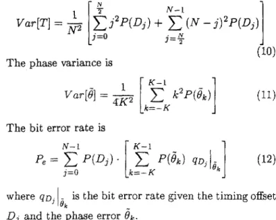
where Threshold is a pre-defined value. Because there exist a stationary steady state, the process converges such that the absolute error in (9) is smaller than the

Threshold value after some iterations. The - d u e of Threshold is dependent on the accuracy of P(&). The timing variance is defined as

N - l

1

The phase variance is

1

The bit error rate is

N - l

r

~ - 1

1

where qo. - is the bit error rate given the timing offset

’

o k

-

Dj and the phase error d k .

4

Simulation Results

In addition to analytical results, the simulation results are presented to justify our work. In our simulation, we assume that the center frequency of the received signal, uc, is 3 MHz, the symbol rate is 1 MHz, and Ad = 0 . 1 . ~ for the phase estimator. I t meam the phase estimator may increases or decreases 0 . 1 . ~ radians from the present estimated phase each time. The signal-t+ noise ratio is defined as

No.

A2T In the simulation, we

consider both sequence length are 32 and 48 symbols with 12 samples per symbol duration. 12 samples per symbol corresponds to 12 MHz sampling rate.

In the analysis, we use the Monte-Carlo with 10000 iterations to obtain the (5) and P i ( & [ D ) because the difficulty of multi-integral. The value of the Threshold in equation (9) is 0.0002. Using the recursive method, the steady state probabilities P ( D j ) , j = 0 , 1 , .

. .

,

( N -

l ) , and P ( & ) ,

k

= - K , - ( K - I), . . .

,

( K - 1) can be obtained. With the equations ( l o ) , ( l l ) , and (12), we can calculate the timing offset, phase error, and the bit error rate.

Figure 4 summarizes the simulation results for sym- bol timing variance and the analytical results according to equation (10). It is obvious that lengthening the se- quence length can improve the timing estimator signif- icantly. When the length of data sequence is changed from 48 to 32, the variance of the timing offset increases about 4 times. The phase estimator has the similar re- sult in Figure 5.

Figure 6 shows the bit error rate of the simulations, the analytical results, and the optimal performance of the bit error rate which is marked with the bound of detection. The analytical results are according to equa- tion (12). In the figure, it is obvious that both the sim- ulation and analytical results are close to the optimal

performance of bit error rate. The reason is that the timing offset and phase error are small which are shown in Figure 4 and Figure 5. In AWGN channel, we can control the sequence length such that the performance of the receiver is asymptotical to the optimum. This shows that our scheme is effective in AWGN channel.

5

Conclusions

An all digital and efficient joint estimator for car- rier phase, symbol timing, and data sequence is pro- posed. The structure is systematically derived by maxi- mum likelihood estimation theory and estimates the pa- rameters recursively according to the decision-directed method. The scheme estimates the symbol timing and data sequence based on the symbol correlators and the carrier phase with Sample-Correlate-Choose- Largest (SCCL) algorithm. The proposed scheme ap- plies the symbol correlator for the calculation of the sequence correlation and symbol detection.

The simulation and analytical results show that the bit error rate of the proposed scheme is asymptotical to the optimal performance in AWGN channel. The vari- ance of phase error and timing jitter can be improved by lengthening the sequence length. But the bit error rate is not so sensitive to the sequence length as the timing variance.

References

[l] H. Meyr and G. Ascheid, Synchronization in Dig- ital Communications vol. 1, John Wiley, 1990. [2] T.Y. Cheng and K.C. Cheng, ”Fully Digital Joint

Phase Recovery, Timing Synchronization, and Data Sequence Demodulation”, submitted to

IE-

ICE.

[ 3 ] P.Y.

Kam,

S.S. Ng, and

T.S.

Ng, ”Optimum Symbol-By-Symbol Detection of Uncoded Digital Data Over the Gaussian Channel with Unknown Carrier Phase,”, IEEE Trans. Commun., Vo1.42, No. 8, pp .2543-255 2; August 1994.

[4]

G.R.

McMillen, M. Shafi, and D.

P.

Taylor, ”Si- multaneous Adaptive Estimation of Carrier Phase, Symbol Timing, and Data for a-49-QPRS DEE Radio Receiver”,

IEEE

Trans. Commun., Vo1.32, No.4, April 1984.

[5] K.C. Chen and L.D. Davisson, “Analysis of a New bit Tracking Loop - SCCL,” IEEE Trans. Com- mun., Vo1.40, pp.199-209, Jan. 1992.

[6] J. G. Proakis, Digital Communications, McGraw- Hill, Singapore.

[7]

S.M.

Ross, Introduction

to

Probability Models, 4ed, Academic Press, San Diago, 1989.

L I

Figure 1:

Branch

structure of the proposed scheme.

'..

-

- Q - - - ~ * ----

2 3 4 5 6

0 1

:-

Pgn4-lo-Nase Ram

Figure

4:

Symbol timing variance.

I --c E D ---.c

T

I

Figure 2: Block diagram of the proposed scheme.

Figure 3: SCCL Structure of the proposed scheme.

091- + 0 8 1 I 0 7c (Sequem Lmgn. Sannple/SSymbol) ' Dmulallon (32.10) o Slnulalion (48.10) . AnWms (32.10) - Anayss (48.10)

Figure 5: Carrier phase variance.

t o 5 m %

.-

An6iyss. (32 12) Andyms (48.12) Bourd 01 Deleclion

;

1 0 6 ₁ UI El 10 ' 2 3 4 5 6 7 8 SgnaI-IDNcise Ratio