Neurofuzzy-model-following control of MIMO nonlinear systems

(1)

Neurofuzzy-model-following

control

of

MIMO

non

I

inea

r

systems

W.-S.Lin and C.-H.Tsai

Abstract: A neurofuzzy logic controller with a compensating neural network and a fine-tuning mechanism in the consequent membership functions is proposed to design the model-following control of MIMO nonlinear systems. The control strategy is developed to facilitate interconnection compensation among subsystems by the compensating neural network and to realise feedback linearisation by online function approximation. By tailoring the fine-tuning mechanism to overcome the equivalent uncertainty appearing within subsystems or as a result of plant uncertainty, function approximation error, external disturbances, or measurement noise, the system is robust to some extent. The overall neurofuzzy control system is proved to be uniform ultimate bounded by using Lyapunov stability theory. Simulation results of a two-link manipulator demonstrate the effectiveness and robustness of the proposed controller.

1 Introduction

Researchers have investigated variant designs of model- following control such as variable structure model-following control (VSMFC) [ 1-31 and adaptive model-following control (AMFC) [4-61. The VSMFC design is capable of achieving a robust controller. But it is based on the restrictive assumption that the ranges of the variation of parameters are known and the resulting control efforts are excessive [7]. The Lyapunov stability method [4], hyperst- ability theory [5], and a deterministic approach [6] were usually considered in the AMFC. These methods can obtain continuous control laws. But for some MIMO nonlinear systems, an adaptive approach cannot guarantee tracking performance or even stability in the presence of unstructured uncertainty or disturbance [8].

In recent years, neural networks and fuzzy logic have been applied to model-following adaptive control [9-131. Jagannathan et al. showed good tracking performance through a Lyapunov stability approach in their model- reference adaptive control using multilayer neural network [13]. Chen and Teng [ l l ] and Kawaji [12] proposed a model-reference control structure of indirect adaptive control type by using fuzzy linguistically system and fuzzy neural network. Yin and Lee [9] designed a fuzzy model-reference adaptive controller by using the fuzzy basis function expansion proposed by Wang [ 141 to repre- sent the parameter information. A robust adaptive law to adaptively compensate the modelling error introduced by fuzzy approximation was constructed in [lo]. The methods mentioned take advantage of fuzzy control systems, ability 0 IEE, 1999

IEE Proceedings online no. 199905 15

DOZ: 10.1049/ip-cta: 199905 15

Paper first received 7th November 1997 and in revised form 10th November 1998

W . 4 . Lin is with the Institute of Electrical Engineering, National Taiwan University, Taipei, Taiwan, R.O.C.

e-mail: weisong@cc.ee.ntu.edu.tw

C.-H. Tsai is with the Institute of Electrical Engineering, National Taiwan University, Taipei, Taiwan, R.O.C.

e-mail: arthur@math.ntu.edu.tw

IEE Proc.-Control Theory Appl., Vol. 146, No. 2, March 1999

to easily incorporate linguistic information into the controller. However, the majority of research effort in this area has focused on nth-order SISO nonlinear systems. For the cases of nonlinear MIMO systems, very few results have been obtained.

In this paper the control of unknown MIMO nonlinear affine systems subject to unmodelled dynamics, bounded exogenous disturbance and measurement noise is addressed. The nonlinear functions in the system are assumed to be completely unknown. A novel design of

neurofuzzy-model-following control is proposed to accom- plish the trajectory tracking of the system. The neurofuzzy logic controller (NFLC) is functionally equivalent to a multilayer fuzzy system cascaded with a compensating neural network. The adjustable weights are meaningful and it can be incorporated with, and directly extracted from, linguistic rules. The proposed scheme has been inspired from previous works [9,10,14,15], and here we extend the application field to MIMO systems. The fuzzy IF-THEN rule used in this paper is a more reasonable one in the sense that it is in the form of “IF situation THEN the control input” rather than “IF situation THEN the value of

some nonlinear function” [9,10,14]. The later rule exists inherently in the plant but is hard to obtain from human expert knowledge. The proposed NFLC consists o f a part for asymptotically nonlinear cancellation and a fine tuning mechanism to take care of the plant uncertainty, approximation error, external disturbance, and measurement noise. The robust property and the convergence of output tracking error are also studied.

2 Problem formulation

Consider an m-input, m-output, n-dimensional nonlinear system governed by

y‘” = f ( x )

+

G(x)u

+

d ( x , t )

(2)

weight-adaptation law

%

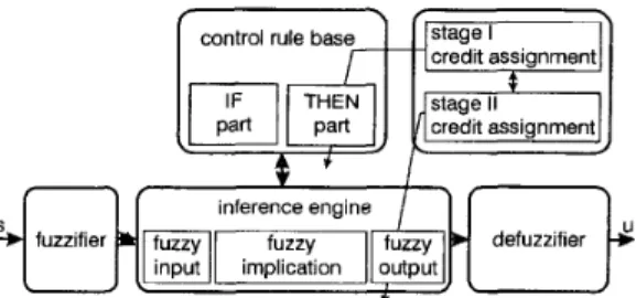
fuuifier reference input V inference engine I defuzzifier

4

reference output

,v

model

Fig. 1 Configuration of proposed neurojuzz,v logic control system

where y = [ y l , .

. .

,y,]? j =

El,

. . . , j m l T , x ( . ) and

X(.)

denote the output, measured output, state and measured state vectors, respectively, y(")

=

[y(ly~),

?P),

. . . , y f i ' ] ? r = [ r , , . . . , r,] denotes the system relative degree, G ( x ) =

. . . ,gln2(.)] are smooth functions, and U = [ u l ,

. . .

, U,] is the system input. The time-varying disturbance d(x, t ) = [dI(x, t), .

.

. , d,(x, t)]? the exogenous signals U,= [v,,~,

.

. , v , , ~ ] ~ and = [vY,, ,

. . .

, vyJT where vy,* E Cri are assumed to have the properties of standard smoothness and boundedness. The zero dynamics equation

C g l ( X ) , ' ' . >$*(X)I>

f(.>

=

v;(.),.

.

'

>fm(.)lT

and g,(.)=

k l l p

li

=

d o ,

Y)

(2)

is assumed to be exponentially stable, or the system is hyperbolically minimum phase. Let y~~ and v, denote the reference output and input, respectively. The aim of control is to make each subsystem of eqns. 1 asymptotically match a linear reference model of the following form

in the presence of bounded disturbance d(x, t ) and meas- urement noise v, and vy. The constants a,1, . . . ,a,,., are selected so that eqn. 3 is asymptotically stable. The control

of such a MIMO nonlinear system poses difficulties, in three main aspects. First the interactions between different subsystems often cause the input applied to one subsystem affecting the other subsystem in an undesirable way. Secondly, the functions G(x), f ( x ) , and q(x), or parameters of the system, may be unknown or difficult to measure. The third one is the disturbance and measurement noise.

Fig. I shows the configuration of the neurofuzzy model following control system. The NFLC, which is formed mainly by cascading a multi-input/multi-output fuzzy system with an adjustable-rule credit assignment unit and interconnections compensating network, is used to approximately cancel the unknown nonlinearity and to decompose the unknown interconnections of the composite nonlinear system into decoupled subsystems. The weights of the NFLC as well as the consequent membership functions of fuzzy rules are directly adjusted by the robust weight-adaptation law and the fine-tuning mechanism to meet some performance specification.

3

controller

Design and analysis of neurofuzzy logic

The MIMO fuzzy-set rule credit assignments (FS-RCA), the interconnections compensating network and the non- singular supervisor are described as follows.

158

3.1 FS-RCA

The configuration of the proposed FS-RCA is shown in Fig. 2. For simplicity, the subscript i of the ith-rule credit assignment for the ith subsystem is omitted by the following expressions. Consider the h z z y rule being of the following form:

RJ: IF xI is A{ AND. '

.

AND x, is A i

THEN U is BJ,j = 1 , . . . , N

+

1 where n

+

1 is the number of fuzzy rules, the antecedent part A L is defined as the following gaussian type

(4)

J 2

$1

A;(%) = exp(-([(x, - cl(k)/akl

I

and the consequent membership function of the consequent part is defined as

(1

+

((CUJ - U ) / a y : > - ' ,

if

U 5 CUJ

(1

+

( ( U - c U J ) / a ; ) b y ,

if

U > c,/

( 5 )

BJ(u) =

where { a i , b i , c&} and { a i , a i , b i , bd, c;} are referred to the premise and consequence parameters, respectively. Given an arbitrary fuzzy input vector A'(x) to the fuzzy system, each rule determines a fuzzy set in the output space U

A'(x) 0 RJ(x, U ) (6)

where 0 represents the compositional operator, and R' ( x , U )

is the fuzzy relation which represents the fuzzy implication. Two rule credit assignment stages are present in Fig. 2. The basic idea of the stage 1 rule credit assignment is to reward good rules by increasing the certainties of the consequent fuzzy sets and punish bad ones by decreasing the certainties of them. After the stage 1 rule credit

control rule b a s e d z l credit assignment

[m*q

1-0

credit assignment

Fig. 2

ble rule credit assignment

Diagrammatic representation of fuzzy system with stage adjusta-

(3)

assignment, the consequent membership function (eqns. 5) is reshaped into (1

+

((CL - U ) / p J a y p , (1

+

( ( U - cC)/pJa;)gR)-', i f U 5 Ck i f U > ck (7) B J ( u ) =

where

fi'

< 1 (or

p J

> 1 ) whenever the rule is rewarded (or punished). The second stage rule credit assignment is imposed on the recommendation fuzzy output of each rule. Giving a credit (aJ to the jth rule refines them and its recommendation output becomes

wJ ' A'(x) 0 Rqx, U ) (8)

where, dot represents multiplication operation and CO' > 1

(or w J < 1) denotes a reward (or a punishment) offered to

the jth rule.

Considering the request of numerical input/output of the fuzzy system, a particular class of fuzzy system with the singleton fuzzified, algebraic product T-norm, the sup star compositional operator [ 141, the local mean-of-maximum (LMOM) [ 161 method and centre average defuzzification are used here. Thus, given input xo = (xy, . . . ,xE), the final output of the h z z y model can be expressed as

where U J is the point in U at which A'(xo)oRJ(x", U')

achieves its maximum value. Using the local mean-of- maximum method, the recommendation output (expr. 6) of each rule is determined by

A'(xo) 0 RJ(x0, U ; ) = Sup [A'(xo)*I(A'(xo),

B'(u))]

U€U

= Z(k(XO), & U ) )

where A'(xo) = A { ( x y ) A? (x;) . . . A: (x!) is the matching degree corresponding to the numerical input xo,

Fl

denotes the location of the singleton implication h z z y set and is defined as

2;

= centroid of { U : E.'(u) 2 Aj(xo)) ₍₁₁₎ Thus, the output response of the FS-RCA becomes

By using eqns. 7 and choosing b/ = b i = 2, expr. 11 can be resolved into

c u - J - - cu .i - pJdLRJ- ₍₁₃₎ where aiR = (af - a1)/2. In the rule base, the (N+ 1)th rule is chosen to be of the Takagi-Sugeno [ 171 type and its consequent membership hnction B"+

'

is singleton with support represented as the form of the synthesis input

(14) CN+l U = Z l j

+

x;

+

'

. .

+

Nrjj(r-')

+

I;

where r denotes the relative degree of the plant. The curvature control parameter of its antecedent membership function

'

is assumed to a roach to infinity so that this rule will be fired whatever x is. The credit assignment takes place in rules RJ, j = 1,

. .

. , N and assigned to be 1 f o ~

RN+

'.

To reduce the number of adaptive weights, /3-' = l i d

is chosen so that credits are assigned simultaneously in BP

IEE Proc.-Control Theory Appl., Vol. 146. No. 2, March 1999

stage 1 and 2. Accordingly, using eqns. 13 and 14, the

analytical formulation of the FS-RCA in eqn. 12 resolves into

uo(t) =

-O(c)Tj@(x)

+

Z"?

+

z$ f .

. .

+

cxrj(r-I)

+

- QL&R<X> W T k " (XI

(15) where 0") andfo(x) are n x 1 column vectors composed of

dc,' and -A'(x), w and go,(.) are ( n

+

1) x 1 column

RCA of eqn. 15, the dehzzification of a multi-inputimulti- output FS-RCA is defined as

U ( ) ( [ ) = P ( X , wJ(-j(x, 0'")

+

U') (16) where

. . . iurn(x) 0 1

L

+

urn - aLK.rn ~ R , m ( x >

1

with

gwi

= [ A ' , . .

.

, A N +

'IT,

wii = . . . , C O ~ + ~ ] ~ ,

d i

is the credit to the jth rule in the ith knowledge rule base, [ - A ' , . . . - A n ] T , andLR,i =

C , " = : ' A J J m .

@(C) = [O""

'

, . . . , yj;y _O/"'O[Oii1 c t i , . . . , _{O i i C U i ]}_{N N T}

1,

_{f o i}A =

3.2 Interconnections compensating network Control of nonlinear MIMO systems with the MIMO FS-RCA directly does not take interconnections among subsystems into consideration, therefore the interconnections compensating network is proposed. By cascading the MIMO FS-RCA with the network, interconnection compensation will occur when the MIMO FS-RCA computes control signals for each subsystem of the composite nonlinear system. The interconnections compensating network maps the out ut of the MIMO FS-RCA, uo, to the control effort uNFtC in the output space U E %", by performing the transformation

U N F L C ( t ) = Mu, = ( I ,

+

W ) u , (18) where I , denotes a m x m identity matrix. The structure of

M reflects that the control effort is combined with uo and its modification to compensate the interconnection of the subsystems. To derive a guaranteed performance weight-

(4)

adaptation law for the NFLC, the algorithm for calculating the weight matrix W is chosen as

3.3 Nonsingularity supervisor

The non singularitynsupervisor_is introduced to monitor the situation of rank

IC)

< rn. If C is found to be singular, it is perturbed as C + [d,], to obtain full rank, where

[d& is a rn x rn matrix with small value component 6,. Then weight matrix W in eqn. 19 is guaranteed to exist. Using eqns. 16, 18, 19 and the matrix inversion lemma, ( A

+

BCD)- =A- (DA- ' B

+

C- ' ) - 'DA-

'

[ 181, the analytical formulation of the NFLC resolves into

- A - ' B

uNFLC ( t ) =

(Z,

-

(Zm

+

ii-'h)-')h-'<-j(x, 0'")

+

v')

= G-'<x, @ ' ~ ) ) ( - j ( X , 0'"')

+

U ' ) ₍₂₁₎ where

&=

c+D, uNFLc t = [uyFLc,.

. .

,U,""""]', and

a'")=

[8$"),

.

. . ,

0iu)]7

Ob(= [ m i l , . .

.

, wim]? Referring

to the NFLC, it seems that G is used to approximate G, and O?)'fei(x) is used to IeamJ infof the controlled plant. If the rough mathematical model and th_e nominal value of the system's parameters are available G can be trained in advance. On the other hand, if expert knowledge for each subsystem presented in fuzzy rule form is provided, the initial weights of the 0"' in the FS-RCA can also be selected at the design stage.

4 Learning algorithm and performance analysis

Define

Bi

= [Bi(C)=, 8i(co)r]T and assume that there exists weights

87,.

.

,e;,

or and

e(")*

such that

where Ef and are small constants. Then eqn. 1 can be

rewritten in terms of the measured output j and the ith component is

160

and

(25)

Afai<x,

vx>

=hi(?)

-foj<.>

A i w i ( x , v x ) = i w j ( ? > - i w j ( x >

are measures of the sensitivity of the nominal model (d(x,

t )

=

U , uy

=

0) with respect to the measurement noise U,. It is then possible to derive the error equation from the ith subsystem of eqns. 23 and 3 as

-ajlyMi

-

aisMi

-

. .

. - a . ir, ~ ' ~ ~ 7 ' ) MI - vi (26) j y

-$j/

= m

+

**Oy)*Tjoi(X)**

+

w,*T~,;(i)uj

+

ii

j = 1 where m

ii

=

[{

+

$Uj

+

d,(x, t )

+

U;,) j = 1

By eqn. 21 subtracting Cy= w i gwi ( i ) u T " and adding

to the right-hand side of eqn. 26, we obtain

fii(i)

+

. . .

+

a . ir

jW1)

I - aLRi&Ri(X)

jl"'

-&/

= ail

6;

- J I M )

+

- j M i )

+

. . .

+

a . rr, @?-I) (ri-1)

+

-

~ ? ) ~ ) j k , ( ? )

- Y M i m or (28) e . I = A . e . I I - b.w. I T e i

+

bi(ci - uLR,i.&R,i)

where ei =

F j

- y M i , j i - j M i , . .

.

, jp - ' ) -y2171)]T and Oi =

8,

- Oi* denote the tracking error vector and weight estimation error, respectively, and

A robust tuning algorithm for

8,

and u L R , ~ motivated by an attempt to modify the basic steepest descent technique and to provide treatment to the exogenous signals, disturbance nd approximation error term

i,,

is proposed in the

!

Q llowing paragraph.

Assumption 1: There exists the smallest non-negative

parameter values 8: 2 0 such that for all

X

E

V

and t E % +

1

5 91 * & R I ( ~ ) (30) Let

Rg,

= {8,(t): lQ1(t)( 5 d1,,,,} be the bounds of

8,,

ail,

be the union of

ne,

and its boundary layer of thickness EO, and

asl

= {&(t): 19,(t)l 5

be the union of

a ,

and its boundary layer of thickness 6s.

The prefix i3 denotes the boundary and = 8,/)8,) is the be the bounds of $,,

(5)

unit normal vector. A smooth robust weight-adaptation law is

if

eTPbbTPe 5 do2 - de,t)ilt)~)R;'[wibirPiei - cT1(Oi - t ) i H ) ] ,

I

otherwise (31) with de, = where satisfj [blr, ' . with R!"'

, b:]: Pi is a symmetric positive-definite matrix . ng the Lyapunov equation AiT Pi+PiAi=- i ,

1.

RiC) and Rj"' are diagonal matrices with positive

diagonal elements and o1 is chosen small but positive constant to keep Oi from growing unbounded. To counter- act the weight estimation errors and disturbances, the control component aLRij&j is employed in the NFLC law (eqn. 21). The parameter of the fine-tuning mechanism

aLRi, which represents the difference between the left and

right spread of the consequent membership functions, is chosen as aLRi ( S i ) = Gi tanh (bir Pi e i h R i ( i ) / E ) where g i is an auxiliary adjustable parameter and E is a small positive constant. ,!Ji is adjusted according to the following adapta- tion laws

the design parameters Qi > 0, Ri = Block diag[R:),

7

with

if

S i [ w : b ~ P l e i - c2(Q

-

So)]

otherwise

Omin[l, dist(S,, M , , ) / E ~ ] , (34)

w I ( ~ )

=ARi(?)

tanh

and cr2 is chosen small but positive constant to keep g i

from growing unbounded.

Theorem I: Consider the nonlinear composite system of eqn. 1 with the NFLC law (eqn. 21), the weight-adaptation laws eqns. 3 1 and 33 operating in the bounded state .Y E Q,.

Then

(i) Oi, gi and the control input uNFLC ( t ) are uniformly ultimately bounded.

(ii) Given any p satisfying p* < p where

p* =

(36)

with Qim=max {Sf, $io} and K being a constant that satisfies IC = i.e. ti = 0.2785, there exists T such IEE Proc.-Control Theory Appl., Vol. 146. No. 2, March 1999

that for Tc t 5 00 the tracking error e converges to the residual set

{ e : eTPe 5 p or eTPbbTPe 5 d i } (37)

Proof Refer to the appendix (Section 9) for details. The overall procedure of the proposed algorithm is summarised as follows.

(i) Specify the design parameters Q,, Rg,, Q,, and Q, based on practical constraints.

(ii) Specify the design constraints E , crl, cr2, r9,, and Ri. Specify a positive definite n x n matrix Qi and solve the Lyapunov equation to obtain a symmetric Pi> 0,

i = 1 , .

.

. ,m.

(iii) Construct the antecedent part A i of the NFLC whose membership function uniformly covers Q, where (iv) Collect the initial centre

CL

and the difference between left and right spread a/Ri of the consequent part BJ rule credit oii and the network weightings oij, i # j , into the vectors Oi and g i , with the constraints that Q i ~ Q , and (v) Apply NFLC (eqn. 21) to the plant, and the robust tuning algorithms eqns. 31 and 33 to adjust the weights Oi and g i .

Remark I : Inspecting the NFLC (eqn. 21), f H (x) and gw,

(x) formed by the antecedent membership function become exact gaussian basis functions that have been proven to be universal approximators. On the other hand, aLRfLRj is seen to be a robust control component and used as a fine-tuning mechanism for encountering approximation errors, disturbance and measurement noise.

Remark 2: It is possible that, during the early stage of learning when if the initial gaussian basis function approx- imations are quite poor, the tracking error might become so large that the plant state would not be in the set Q,. To obtain a global stable strategy subject to the mentioned situation, a nonlinear control methodology known as supervisory control [14, 19, 201 can be used to drive x toward Q, at this time. Moreover, the smooth integration of the NFLC and the supervisory control can be not only a globally stable solution to the tracking problem, but also a guidance to specify parameters such that the control U are within the constraint sets, 0, [14].

Remark 3: It is interesting to observe that the parameter

matrices R!", and

I?!'")

in Ri represent the inverses of the learning rate of 0;'' and Oi'"', respectively. For instance, suppose the variations of the components of G being smaller than those off, then the learning rate of 0:") can be chosen smaller than that of @'), and vice versa. This

provides a guideline to design the parameters.

Remark 4: From eqn. 36 the tracking error residual is determined by the design parameter p*. If the design constants E , 0 1 , 0 2 , rg,, R i , Qi and Pi are appropriately chosen, it is possible to make p* as small as desired and therefore better tracking performance can be achieved.

Remark 5: The initial designs of Oio and $io in the NFLC can be considered as initial estimates of the best weights 0: and

$7

respectively. The closer Oio and to t)T and

$T,

respectively, the smaller p* becomes. This, in turn, results in better tracking.

Remark 6: Suppose that some partial knowledge about the

dynamic system to be controlled are known in the form of "approximation to f ( x ) " and "approximation to G(x)" denoted by the terms

f"

(XI

nominal system parameters) k= 1 , .

. .

, n , j = 1 , . . . , n

+

1.

9j E

n,i.

(6)

and

@

(XI

nominal system parameters), respectively.

Then a set of initial weights 06“’ and Oba) can be selected

by using the well-known least square (LS) algorithm, etc., such that Ojo will be close to

St

and small p* can be achieved.

5 Simulation

Consider a two-link robot manipulator, which was also investigated in [ 3 ] , characterised by

(ml

+

m 2 > 4

+

m2<

+

2m2rlr2~2

+

J I m 2 4

+

m2r;

+

m2rlr2c2 m2r:

+

J2

( 3 8)

where m l , 1112, J , , J2, r l = 0.511, and r2 = 0.512 are the mass, the moment of inertia, the half length of link 1 and 2, and

c 1 cos(ql), s12 sin(ql

+

q 2 ) , etc. For comparison, com- puter simulations have been conducted with conditions the same as used in [ 3 ] . The inertia parameters are chosen to be ZI = 2.0 m, 12 = 1.6 m, J 1 = J2 = 5.0 kg

.

m, m l = 0.5 kg, and m2 = 6.25 kg, and the trajectories to be followed are

described by two decoupled linear systems as

ijMj = ail qMj

+

ai2qMj

+

vi, i = 1 , 2 . (3 9) Their responses are shown in Fig. 3. The model parameters and the driving inputs are chosen to be ail = ai2 =

-

1,

i = 1 , 2 and u1 = v2 = 1 , respectively. The situation char-

acterised by the same initial conditions on the reference model and the plant are considered. The values are set to be

q l ( 0 ) = - 1.57 rad, q 2 ( 0 ) = 0 rad, q1 ( 0 ) = 0 rud/s, q2(0) =

0 rud/s. The membership functions of states q l , q l , q2, and

q2 (represented by generic variable x i ) for the qualitative statements are defined as {NB, NS, ZE, PS, P B ) where NB:

A&) = exp(-4(xi

+

l.8)2), NS:Aj(x,)=exp(-4(xi+0.8)22),

ZE: A&) = exp(-4~?), PS: A&) = exp(-4(xi - 0.8) ),

PB: A i ( x j ) = exp(-4(xi - 1.8)’). The elements in G I t ) and are chosen randomly within the interval (- 10, 10) and ( - 2 , 2), respectively. In eqns. 31 and 33, the design parameters are given by Q , = Q2 = 101, 2, R 1 =Block diag [0.011625 x 625, 320001625 x 6 2 5 , 20000~625 x 6251, R2 =

Blockdiag L0.0251625 x 625,200001625 x 6 2 5 , 320001625 x 6251,

oI = 0.002, g2 = 0.001, and 8 = 0.005. Two sets of simula-

tion results are in order.

1.6 I I I I

-1.6

0 2.5 5.0 7.5 10.0

timet, s Fig. 3 Reference outputs ofjoints

__joint 1 . . . . . . joint 2 162 0.060

3

0.050 0.040 0.030 0.020 0.01 0

p

o

g

-0.010

I

I I I

I

-

? 0.006 E 0.005 0.004 0.003 0.002 0.001 0 -0.001 -0.002 -0.003 -0.004 -0.005 0 2.5 5.0 7.5 10.0 timet, s b Fig. 4 a Joint 1 b Joint 2

Trucking errors ofjoints U

5. I Tracking without measurement noise

Fig. 4 shows the results of simulation without considering measurement noise. It depicts that the robot tracks the desired trajectory nicely, and the NFLC performs much better in terms of accuracy, in comparison with the adaptive variable structure model following control (AVSMFC) scheme [ 3 ] .

5.2 Tracking with measurement noise and torque disturbance

In this simulation the combined effects of the friction and the external torque disturbances given as

d , = 2.0 sin(q,)

+

2.5 sin(q2)

+

0.5 sin(t) d2 = 5.0 sin(q,)

+

4.0 sin(q2)

+

0.4 sin(t)

and the measurement noise are applied. The noise are assumed to be white with uniform distribution within

[-0.01, 0.011 (rad). The effects of noise of different sensors are assumed to be independent of each other. The simulation results are depicted in Fig. 5. It is well known that even a small measurement noise can affect significantly the stability of a control system [8]. But in the proposed NFLC-based control, by tailoring the fine-tuning mechanism to overcome the equivalent uncertainty, the system is shown to be stable in the presence of both measurement noise and disturbances. This agrees with our analytical result (theorem 1).

(40)

5.3 Tracking with reinitialisation error and prelearning

In Fig. 6 the reinitialisation errors are set as ql(0) - q m l ( 0 ) =- 0.05, and q2(0) - qm2(0) = 0.05. The simula-

tions are conducted for cases with and without prelearning by using the rough mathematical model and nominal IEE Proc.-Control Theory Appl.. Vol. 146, No. 2, March I999

(7)

U E 9 5

P

L” P E 4.4 Fig. 5 U E L

-g

P

i ?₊ Fig. 6 0.040 0.030 0.020 0.010 0.060 0.050

-

0.060 0.050 0.040 0.030 0.020 0.010 -0.010 -0.020 -0.030 -0.040 I I I

-

0~

-

I I

Tracking errors of joint I and 2 with measurement noise

0.060 0.050 0.040 0.030 0.020 0.010 - I I

-

-0.010

‘

I I 1 I 0 2.5 5.0 7.5 10.0 timet, s b

Tracking errors ofjoint I and 2 with reinitialisation error without prelearning with prelearning

a Joint 1

b Joint 2

parameters of the robot manipulator. The nominal parameters are chosen as

1 ~ = 2 . 2 m , 1 ~ = 1 . 4 m , J ~ = 4 . 8 k g ~ m , J ~ = 5 . 1 k g ~ m , m ~ = 0.48 kg, m; = 6.30 kg

When the robot’s nominal parameters are known a priori

through the application of the training data {x(k)}, the

initial weights Of’ and

Op)

are chosen based on IEE Proc-Control Theory Appl.. Vol. 146, No. 2, March 1999

element-by-element minimisation of the following objec- tive function

I[fo(x(k)lnominal robot parameters) -?(A?), Ob‘’)

[I2

IIGo(x(k)(nominaZ robot parameters) - Ol;“’)l12

32 testing points from either along the desired tra’ectories

or near them are chosen as the training data {x (Jk) }. The dash and solid lines show ‘respectively’ the simulation results of the NFLC with and without a priori knowledge

of the robot’s nominal parameters. It is obvious that the prelearning one obtains much better tracking performance.

k

6

Conclusion

Two novel approaches have been introduced into the design of neurofuzzy logic controller for the model following control of unknown MIMO nonlinear systems. A compensating neural network is used to deal with the interconnec- tions of composite nonlinear systems. A fine-tuning mechanism in the consequent membership function is developed to obtain the robust property. It has been proved that the overall neurofuzzy control system is able to guarantee the output tracking error to converge to a residual set ultimately. The simulation results of robot control show that the proposed NFLC can be trained automatically to give a satisfactory model-following performance, and the system is robust to the disturbance and measurement noise.

7 Acknowledgments

The authors are indebted to the anonymous referees for their valuable comments. The authors would also like to thank Dr. Jing-Sin Liu for his helpful suggestions and comments. 8 1 2 3 4 5 6 7 8 9

References

GUZZELLA L., and GEERING H.P.: ‘Model following variable structure control for a class of uncertain mechanical systems’. Proceedings of 25th IEEE Conference on Decision and Control, 1986, 3, pp. 3 12 -3 16 YOUNG K.-K.D.: ‘A variable structure model following control design for robotic application’, IEEE Truns., 1988, RA-4, (5), pp. 556-561 LEUNG T.P., ZHOU Q.J., and SU C.Y.: ‘An adaptive variable structure model following control design for robot manipulators’, IEEE Trans.,

DUBOWSKY S., and DESFORSES D.T.: ‘The application of model referenced adaptive control to robot manipulators’, Trans. ASME 1 Dyn. Syst., Meas. Control, 1979, 101, pp. 193-200

BALESTRINO A., DEMARIA G., and SCIAVICCO L.: ‘An adaptive

model following control for robot manipulators’, Trans. ASME 1 Dyn. Syst., Meas. Control, 1983, 105, pp. 143-152

SINGH S.N.: ‘Adaptive model following control of nonlinear robotic systems’, IEEE Trans., 1985, AC-30, (3), pp. 1099-1 100

AMBROSIN0 G., CELENTANO G., and GAROFALO F.: ‘Tracking control high-performance robots via stabilizing controllers for uncertain systems’, 1 Optim. Theovy Appl., 1986, SO, pp. 239-255

REED J.S., and IOANNOU P.A.: ‘Instability analysis and robust adaptive control of robotic manipulators’, IEEE Trans., 1989, RA-5, 1991, AC-36, pp. 341-353

(3);pp. 381-386

YIN T.K., and GEORGE LEE C.S.: ‘Fuzzy model-reference adaptive control’, IEEE Trans. Syst., Man, Cybern., 1995,25,(12),pp. 1606-1615 10 CHEN C.S.. and CHEN W.L.: ‘Robust model reference adaptive control of nonlinear systems using fuzzy systems’, Int. 1 Svst. Sci., 1996, 27, (12) pp, 1435-1442

11 CHEN Y.C., and TENG C.C.: ‘A model reference control structure using a fuzzy neural network’, Fuzzy Sets Syst., 1995, 73, pp. 291-312

12 KAWAJI S.H.: ‘Model following servo control for fuzzy linguistical systems’. Proceedings of IEEE Conference on Fuzzy Systems, 1996, 2,

pp. 1420-1426

13 JAGANNATHAN S., LEWIS EL., and PASTRAVANU 0.: ‘Model reference adaptive control of nonlinear dynamical systems using multilayer neural networks’. Proceedings of IEEE Conference on Neural

Network, 1994, 7, pp. 41664171

14 WANG L.X.: ‘Stable adaptive fuzzy control ofnonlinear systems’, IEEE

Trans. Fuzzy Syst., 1993, 1, (2), pp. 146-55

(8)

15 POLYCARPOU M.M., and IOANNOU P.A.: 'Robust adaptive nonlinear control design', Automatica, 1996, 32, (3), pp. 4 2 3 4 2 7

16 BERENJI H.R., and KHEFKAR P.S.: 'Learning and tuning fuzzy logic controllers through reinforcements', IEEE Trans. Neural New., 1992,3, ( 9 , pp. 7 2 4 7 4 0

17 TAKAGI T., and SUGENO M.: 'Fuzzy identification of systems and its applications to modeling and control', IEEE Trans. Syst., Man, Cybern.,

1985,15, pp. 116-132

18 HORN R.A.. and JOHNSON C.R.: 'Matrix Analysis' (Cambridge University Press, Cambridge, UK, 1985)

19 SANNER R.M., and SLOTINE J.-J.E.: 'Gaussian networks for direct adaptive control', IEEE Trans. Neural Netw., 1992,3, ( 6 ) , pp. 837-863

20 TOVORNIK B., and DONLAGIC D.: 'How to design a discrete super- visory controller for real-time fuzzy control systems', IEEE Trans. Fuzzy S y ~ t . , 1997, 5, (2), pp. 161-166

9

Appendix

9.1 Proof of theorem I

Let VQ and V , be positive-definite functions of the forms Vo

=.iCL1(HTdi),.

-V, =

i,Csl

g2. Their time derivative are Vo = OTO, and

v,

=

ELl

$Tji,

respectively. If the first line of eqn. 32 is true, then do,=O and the conclusion

Po

5 0 is trivial. If the second line ofeqn. 32 is true then do, < 1 and Bi E

Riz.

Therefore either Vo 5 0 or B i ~ R i L is obtained. Similarly, either

Vg

< 0 or & E

Rg,'.

Therefore the boundedness of

Bi,

&,

and uNFLc is guaranteed. To show the performance of the closed-loop system formed by eqns. 1 , 2 1 , 3 1, and 33, we choose the following positive-definite functions:

v =

V , + . . . + V * (38) where i d :

+

i @ R i e i

+

f r 9 , $ ,

1

eTPiei

+

@Rigi

+

4

r8,

@,

if

eTPbbTPe

5 d: otherwise (39) q t ) =

si(t) = si(t)

-

$?

are the auxiliary adjustable parameter error and gim

=

max

**{si*,**

Taking the derivative of V, along the trajectories of the closed-loop system and taking e ns. 28, 31, and 33 into account we obtain

5

= 0 for

9

e

Pbb' Pe

5 d i , and

c(t) = erPi(Aie, - bi@w

+

bi(ci - aL,j&>>

+

er(r

- d o O i l B ~ ) [ w b ~ P , e , - o,(o, -

e,,)]

+

j i ( l - dg)[wibrPiei - 02(gi -

+

i3fwbrPiei - ol@'(Oi

-

eio)

+

9 . i w ~ b ~ p j e i

- a29.i(9i -

- d&8,,0~[wbrPiei -

al(ei

-

eio)l

= feT(ATP,

+

PjAi>ei - eTPjbL@w

+

eTp,bi(ci - g,w:>

-

i T

- dggi[wibi Piei

-

02(gi - Sio)]

(40) for

eTPbbTPe>

do2. By eqn. 32, if

ei',

[w,b~P,e, - o1

(ei

-

O i O ) ] _< 0, we have de,= 0 and the last term of the preceding equation is equal to zero. When O;, [wjbTPi ei - ol(8i - Bio)] > 0, if di E we also have do, = 0 and the conclusion holds. If Bi$R0, and suppose that Rg, and

R-9, are appropriately selected such that

Op

and

SF

are in the interior of 00, and 0 3 , respectively, we have

ereil

=

(e,

-

eT)Te,/leil

=

+[(e,

-

@?)'(e,

- 07)

+

ere,

-

etTey/lejl

2

o

(41)

or

In a similar way we can show that

Using assumption 1, the second term on the right-hand side satisfies the inequality

where K is a constant that satisfies K =e-("+ I ) , i.e. K =

0.2785. Since the following fact can be shown easily by straightforward algebraic manipulation.

Claim 1

(46) 0 5 - y tanh

(3

- 5 K E

for any y E R . Furthermore it can be readily shown that

6T(oi

-

e,,,)

=

;e;e,

+

i(oi

-

eio)T(ei

-

eio)

-

;(e:

-

e,o)T(e?

-

e,)

5i(9i - 9'0) =

4 5;

+

$ ( S i - gi0)* - $(Si* - (47)

Hence

V . < --e'(Q:)e. 1

-"'ere.

-si?

2 2 " 2 I

2 2

I -

o M

+

-

eio)T(BT

- Oi0)

+

A($?

-

+

si

ICE

-

< -aiV, + A i (48)

where

and

cr. o M

i, '= 2

(e;

-

eio)T(BT

-

e;,) +

2

($T

- g i 0 y

+

$i K & or

V s - a V + I (49)

where a = min ai and

I = E y = l I i .

The differential inequality (e&. 49) satisfies

Therefore ei(t),

el,

g i are uniformly ultimately bounded. Let p* = 2 2 a then from expr. 50 we readily obtain expr. 37.