演化式基因演算法應用於平行測驗之建構
An Evolutionary Genetic Algorithm for Parallel Test Construction
Koun-Tem Sun1, Yi-Chun Lin2 , Yueh-Min Huang2*
1Dept. of Information & Learning Technology 2 Dept. of Engineering Science
National University of Tainan, Taiwan National Cheng Kung University, Taiwan [email protected] [email protected]
Abstract
In this paper, we proposed a new approach called “evolutionary genetic algorithm” that improves the efficiency and the quality of the simple genetic algorithm (GA) in constructing parallel tests.
The basic principle of this evolutionary genetic algorithm combines two theories. One is that of genetic diversity, which is beneficial to species evolutionary existence. The other is eugenic theory, which can increase the probability of finding better offspring. Experimental results show that our approach is much better than the simple genetic algorithm in terms of time efficiency and solution quality. The evolutionary genetic algorithm would be a more powerful tool than the simple genetic algorithm for parallel test construction.
Keywords: genetic algorithm, parallel test construction, time efficiency, solution quality.
本研究將提出一新的演算方法”演化式基因 演算法(evolutionary genetic algorithm)”應用於平 行測驗建構上。此演算方法主要結合兩個概念:即 生 物 多 樣 性 (genetic diversity) 以 及 優 生 學 理 論 (eugenic theor)。自然界中,生物多樣性有利於物 種演化綿延不絕;優生學概念則強調產生更佳的下 一子代。結合這兩個概念於本研究所提出之演化式 演算方法,其實驗結果顯示,此演算方法比起傳統 基因演算法具有更高的效率以及得到更佳的解。同 時也證明此演化式基因演算法將成為平行測驗建 構更有效的工具。
關鍵詞:基因演算法,平行測驗建構,時間效率,
解答品質
1. Introduction
In the past decades, test construction methods (Lord, 1953; Lord & Novick, 1968; Lord, 1980;
Weiss, 1982; Hambleton & Swaminathan, 1985;
Theunissen, 1985; Baker, Cohen, & Barmish, 1988;
van der Linden & Boekkooi-Timminga, 1989) were simple and inflexible due to the lack in popularity of personal computers. Recently, related research (Luecht & Hirsch, 1992; Stocking, Swanson, &
Pearlman, 1993; Armstrong, Jones, & Rutgers, 1996;
Armstrong, Jones, & Kunce, 1998; van der Linden &
Adema, 1998; Csöndes & Kotnyek, 2002; van der Linden, 2005; van der Linden, Ariel & Veldkamp, 2006) has proposed various techniques and methods on test construction successfully due to improvements in the efficiency of computers.
However, since test construction is an NP-hard problem (van der Linden, 1998), the execution time presents exponential growth with growth in problem size. An efficient technique is still required to find better solutions. The genetic algorithm is based on the Darwinian Theory that has a powerful ability to find the optimal or near optimal solutions from a huge pool (Goldberg, 1989), and has also been designed to solve the parallel test problem (Sun, 2000), obtaining very good results. In this paper, we combine genetic diversity (Fisher, 1930; Hubbell, 2001) with eugenic theory (Barrett & Kurzman, 2004) to improve the efficiency and quality of the simple genetic algorithm for parallel test construction.
First, we briefly introduced the concept of parallel test construction by the simple genetic algorithm. To solve the parallel test construction problem by a genetic algorithm, we first transformed this problem into an optimized form. The formula of test information function can be represented by a linear math model as follows.
Maximize j i
n
i i
j
I θ x
O ( )
1
∑
==
, (1)Subject to
,
q'
Cq i
i q i
q
A x k
k ≥ ∑ ≥
∈
, q=1 ~ p, (2)
where p is the number of total constraints, Ai,q is the qth content attribute value of item i, Cq is the qth
constraint and kq and
k
'qare the constraint values.When we want to construct a test, Eq. (1) would be maximized and would satisfy all constraints (Eq.
(2)). However, in the construction of parallel tests, several tests need to be constructed and the deviation between them (the sum of squared errors) needs to be minimized. If we choose one of the parallel tests as a standard (denote by dj ), then the other test information (denoted by Oj) of the two parallel tests should have the minimum deviation from the standard test by using the following equation.
Minimize ( )2
1
j s
j
j O
d E =
∑
−=
(3)
Equation (3) would be used in the fitness function of the genetic algorithm.
The detailed steps of applying a genetic algorithm to create parallel tests can be described as follows.
First, set the initial population of chromosome strings X. Each chromosome string X k represents a constructed test k, which contains n bits (n is the number of items in the item bank), among which, m bits are 1 and the rest are 0, for a test with m items.
Each bit x represents whether an item is included i or not in the test (x =1i , Yes;x =0 , No). For each i chromosome, we can calculate the fitness function as follows:
, ) (
)
( 2
1
k j s
j j
k d O
X
fitness =
∑
−=
(4)
where Okj is the value of the test information function at ability level j for the kth parallel test. The lower the fitness value (deviation) is, the better the result obtained. When constraints are considered, the fitness(Xk) is modified as in Equation (5):
fitness(Xk) = fitness(Xk) + r, if r of p
satisfie , or , q'
C i
i q i q
C i
i q
i x k A x k
A
q q
<
>
∑
∑
∈∈
(5)
where r is the number of constraints which have not satisfied the constraints in Equation (2). Then, complete the following genetic operations for generating P offspring from current chromosomes in the population.
(1) Two-point crossover operation: two offspring for each pair of parents are generated with the probability pc. A section of the chromosome string in the offspring is the same as one parent and else is the same as the other parent.
(2) Two-point mutation operation: randomly select
some chromosomes with probability pm from the population and randomly choose two positions.
Mutation occurs when 0 is changed to 1 and 1 is changed to 0 in the selected chromosome, and it then becomes the offspring.
(3) Reproduction operation: the best chromosome string is found in the “parent” population having the reproduction probability pr. These then become the offspring which make up the new population (also called elitism selection).
Repeat the above steps (1) ~ (3) for generating n new chromosomes (tests) and replace the old ones in the population until a generated chromosome (solution) fits the expected result or the number of generations reaches the predefined value.
Finally, a chromosome (test) with the minimum deviation within the population would be the solution of the parallel test construction problem.
The simple genetic algorithm can deal with parallel test construction simply and easily with constraints and obtain very good results, but the efficiency and quality could be improved by the further inclusion of some useful theories. In this paper, we propose an “evolutionary genetic algorithm” to improve the test quality of evolution which combines two theories, genetic diversity and eugenic theory.
In a natural life system, there are similar or different characteristics making up each individual.
This variation is the meaning of bio-diversity or polymorphism (Fisher, 1958). In general, bio-diversity is the basic characteristic of a life system, but diversity does not arise from natural selection. Most of the time, crossover and mutation are important processes in creating genetic diversity.
Therefore, genetic diversity in the interlocking nature of the system guarantees species continuous evolution in natural selection and the species should evolve to fit with its environment more easily (Fisher, 1930).
We will apply the concepts of the above-mentioned theories to the simple genetic algorithm. The basic concept is to examine the diversity between two new offspring and compare that against the diversity between the new offspring and the chromosomes included in population. If the diversity was greater than the threshold value, then the new offspring would be selected into the population. Else, the offspring is eliminated through competition. As a result, it ensures the diversity of intra-population in the environment. Corresponding this to the parallel test construction problem, we can find a set of tests having the greatest difference to find the best parallel test form.
According to eugenic theory, there is a higher probability of generating better offspring if two of the better individuals are selected to mate (Barrett &
Kurzman, 2004). Therefore, we can find better results efficiently if we select only the better individuals to
mate at each evolutionary generation. The concept is similar to selecting the stud in animal husbandry.
However, the local minimum often occurs during the evolutionary process.
We have, therefore, incorporated the advantages of these two theories into the simple genetic algorithm. Experimental results show that our proposed method can construct parallel tests with a smaller margin of error than the simple genetic algorithm.
2. Evolutionary genetic algorithm for parallel test construction
To verify the effectiveness of our evolutionary genetic algorithm, we first compared the performance of three techniques: genetic diversity, eugenic theory, and the mix of genetic diversity and eugenic theory.
The concept of each technique as applied to parallel test construction is stated as follows.
(1) Genetic Diversity Method (GDM): The items selected for inclusion in each test are as far as possible different. Each test is represented by a one dimensional chromosome which is selected to evolve for the next generation when the distance between it and tests already included in the population is great enough (i.e., the distance beyond a predefined threshold value). This technique generates a set of offspring (tests) of the greatest difference for evolution.
(2) Eugenic Theory Method (ETM): This technique considers only the fitness value of each test (offspring). Tests with the smaller number of errors would be selected to mate by the crossover operation generating two new tests (offspring) which have a higher probability of finding the better solutions.
(3) Evolutionary Genetic Algorithm (EGA): This approach combines the above two techniques, GDM and ETM. In the first half of the execution of EGA, we apply the GDM which makes the chromosomes (tests) as diverse as possible in the initial evolution thus avoiding having the results fall into a few local optimal solutions. Then, the selection pool is made as wide as possible by the genetic diversity method in the first half of the process of evolution. After the first half of the process, we apply the ETM to search for the optimal solution from a set of better solutions (candidates) to in turn evolve better offspring in the next generation. Then, optimal or near optimal solutions would be generated rapidly.
The detailed execution of the steps of each approach to parallel test construction is stated as follows.
(1) Genetic Diversity Method
The principle of GDM is based on the concept of the genetic diversity of nature. In nature, diversity is critical for the stable existence of a species. In other words, individuals need to maintain a degree of variation (diversity) to confront challenge for natural
selection (Endler, 1986). So if we maintain the diversity of selected items during the selection process, it is useful in finding various combinations of items for test construction.
For reaching genetic diversity, the selection process of two generated offspring after the crossover operation of the simple genetic algorithms is designed as follows.
(1) When two offspring are both infeasible solutions, neither of them is selected into the population for the next generation; (2) when one offspring is a feasible solution and another is an infeasible solution, the selection is made by computing the distance between the feasible solution and other selected solutions in the population. If the distance is greater than the predefined threshold value, then this offspring is included in the population for the next generation; (3) when two offspring are both feasible solutions, we first compute the distance between the two offspring.
If the distance is less than the threshold value, then the distance of the offspring with the greater distance between it and other selected solutions would be computed. This offspring is then selected into the population if the computed distance is also greater than the threshold value. If the distance between the two offspring is greater than or equal to the threshold value, then the distance between each one of the offspring and other selected solutions is computed.
The offspring is selected into the population if this distance is also greater than the threshold value. The algorithm of GDM could be stated as follows.
/* The selection process of GDM for two offspring
'
P
1 andP
2' after the crossover operation of GA */(1) Set the threshold value of distance: dθ. (2) Selecting offspring
P
1' orP
2'(2.1) if
P
1' andP
2' are both infeasible then regenerate two offspringP
1' andP
2'(2.2) if only
P
1' (orP
2') is feasible thencompute the distance between
'
P
1 (orP
2') and other solutionsP
k in population P
∈
∀
= P P
kP
kd
1minmin{ distance (
1', ),
P}
∈
∀
= P P
kP
kd
2minmin{ distance (
2', ),
P}if
d
1 min(ord
2 min) ≥ dθ then selectP
1'(orP
2')else regenerate offspring
P
1' andP
2'(2.3) if
P
1' andP
2' are both feasible thencompute the distance d12 between
P
1'and
P
2'compute the distance
d
1 minbetween
P
1' and other solutionsP
kin population Pcompute the distance
d
2 minbetween
P
2' and other solutionsP
kin population Pif d12 < dθ
then if
d
1 min >d
2 min and1
d
min≥ dθ then selectP
1' elseifd
2 min ≥d
1 min and2
d
min≥ dθ then selectP
2'else regenerate offspring
'
P
1 andP
2'if d12 ≥ dθ
then
if
d
1 min≥ dθ then selectP
1'if
d
2 min≥ dθ then selectP
2'if
d
1 min< dθ andd
2 min< dθthen regenerate offspring
P
1' and'
P
2(2) Eugenic Theory Method
The concept of the eugenic theory method is to select the better solutions into the population such that there is a higher probability to generate better offspring after the crossover operation. However, the probability of trapping at local minimum is also increased. The selection process for two offspring by the ETM is designed as follows. (1) When two offspring are both infeasible solutions, neither of
them is selected into the population; (2) when one offspring is a feasible solution and another is an infeasible solution, select the feasible (better) solution into the population; (3) when two offspring are both feasible solutions, select the better (smaller fitness value) one into the population. The algorithm of ETM could be stated as follows.
/* The selection process of ETM for two offspring
'
P
1 andP
2' after the crossover operation of GA */if
P
1' andP
2' are both feasiblethen select the smaller of
P
1' andP
2'elseif only
P
1' (orP
2') is feasible, then select the feasible solutionP
1' (orP
2')else regenerate offspring
P
1' and'
P
2(3) Evolutionary Genetic Algorithm
This method combines the advantages of the genetic diversity method (GDM) and eugenic theory method (ETM). Initially, we adopted the genetic diversity method to search a wide ranging problem space and in this way avoided falling into localized optimal solutions. Then, we expanded the search space making it as wide as possible in the first half stage. Now, after the search for diversity, we apply the eugenic theory method and select better solutions to continue the intensive search for the optimal solution regardless of diversity any more (e.g., if the number of generations was set to 1000, then the first 500 generations would adopt GDM, and the last 500 generations would adopt ETM). In this way, we consider both genetic diversity and eugenic theory and obtain results that were better than the simple GA.
The algorithm of EGA could be stated as follows.
/* The selection process of EGA for two offspring
'
P
1 andP
2' after the crossover operation of GA */(1) Initially, set gener_no to 1 (2) Repeat
if gener_no < 1/2 generation_number /*
gener_no is the index of generations */
then apply the GDM else apply the ETM gener_no = gener_no + 1
Until gener_no = generation_number
3. Performance comparison
To compare the performance of the proposed three techniques, we used a computer to generate a virtual 1000-item bank. The parameters of each item are randomly generated and their scopes are shown in Table 1.
The parameters set for evolution were defined as follows: n = 1000, m = {30, 40, 50}, P = 100, pc = 86.3%, pm = 0.4%, pr = 13.3%, gener_no = 300 ~ 5000, and dθ = 6.
For experiments of 300-generations, EGA had the least number of errors in 5 out of 9 cases, and ETM had the least number of errors for the remaining 4 cases (as shown in Table 2).
From Table 2, we can see that the ETM and EGA techniques obtained similar results. For further comparison of these two methods, more experiments proceeded with the number of generations changing from 300 to 5000. Simulations were divided into two parts. The first part (PART 1) included cases generated by ETM that were better than those of EGA at 300 generations (shown in Table 3). The other part (PART 2) composed the remaining five cases (cases generated by EGA that were better than those of ETM (shown in Table 4)).
From experimental results, we found that the proposed EGA method obtained the best results among the three proposed approaches. We will now compare it with the previously proposed SGA method (Sun, 2000) of parallel test construction.
4. Performance Evaluation
In this section, we will compare the performance of EGA and SGA to verify the hypothesis that combining genetic diversity and eugenic theory into the SGA is useful for evolving better solutions. Nine hundred target tests were randomly generated by computer, and results were generated by the execution of EGA and SGA, respectively.
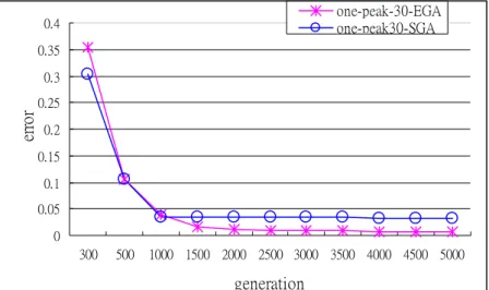
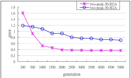
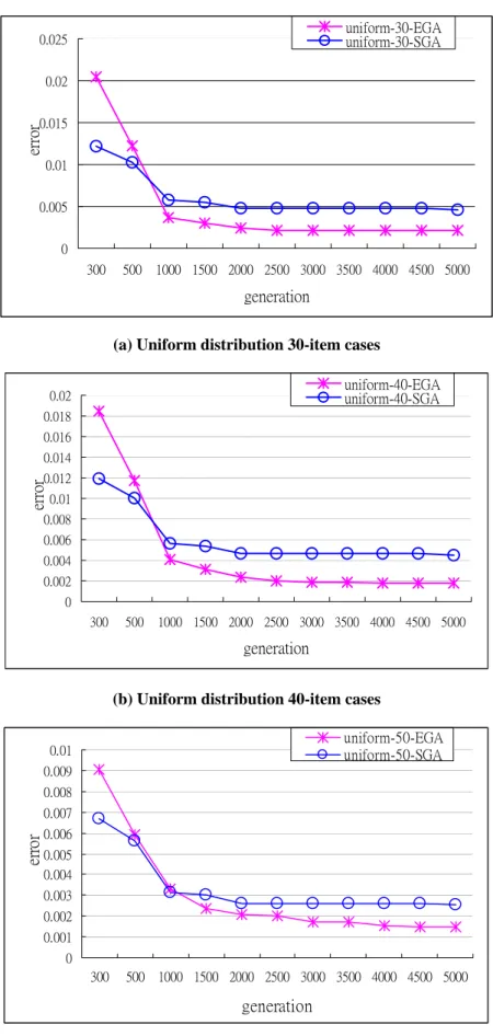
Figure 3 (a) ~ (c) shows that in one-peak cases EGA had better solutions if the number of generations was beyond 1000. Figure 4 (a) ~ (c) shows that in two-peak cases EGA had better solutions if the number of generations was beyond 500. Figure 5(a) ~ (c) shows that in uniform distribution cases EGA had better solutions for 30-item and 40-item cases if the number of generations was beyond 1000 and for 50-item cases if the number was beyond 1500. Figures 3 ~ 5 also show that SGA often got trapped in a local minimum (horizontal periods of lines). Then, the results were worse for larger generations. Experimental results satisfied our postulation that the combination of genetic diversity and eugenic theory is useful for evolving better results.
5. Conclusions
This paper proposed three techniques, GDM, ETM, and EGA, to improve the performance of the simple genetic algorithm. The basic principles behind these techniques are: genetic diversity, eugenic theory, and the mixing of the two. Based on the constructed 1000-item bank, 900 different target tests were simulated to compare the performance of these three
techniques. Experimental results show that the EGA had the best performance for the cases with the larger number of generations. Then, another 900 different target tests were used to compare the performance of EGA and SGA, and the EGA was also better than the SGA after a large number of evolutionary generations.
The phenomenon confirmed our hypothesis that “the combination of genetic diversity with eugenic theory could improve the performance of SGA.” The proposed evolutionary genetic algorithm would be more effective in parallel test construction than the SGA.
In the future, we will reinforce our method and expect to solve more complex problems such as item duplication and item exploration.
Acknowledgments
This research was supported by the National Science Council of Taiwan, ROC, under the grant NSC 93-2520-S-024-004-.
6. References
[1] Armstrong, R. D., Jones, D. H., & Kunce, C. S.
(1998). IRT test assembly using network-flow programming. Applied Psychological Measurement, 22(3), 237-247.
[2] Armstrong, R. D., Jones, D. H., & Rutgers, X.
L. (1996). A study of a network-flow algorithm and a noncorrecting algorithm for test assembly.
Applied Psychological Measurement, 20(1), 89-98.
[3] Baker, F. B., Cohen, A. S., & Barmish, B. R.
(1988). Item characteristics of tests constructed by linear programming. Applied Psychological Measurement, 12(2), 189-199.
[4] Barrett, D., & Kurzman, C. (2004). Globalizing social movement theory: The case of eugenics.
Theory and Society, 33(5), 487-527.
[5] Csöndes, T., & Kotnyek, B. (2002). Greedy algorithms for the test selection problem in protocol conformance testing. Journal of Circuits, Systems & Computers, 11(3), 273-281.
[6] Endler, J. A. (1986). Natural selection in the wild. New Jersey: Princeton University Press, Princeton.
[7] Fisher, R. A. (1930). The genetic theory of natural selection. Oxford: Oxford University Press.
[8] Fisher, R. A. (1958). Polymorphism and natural-selection. Journal of Ecology, 46(2), 289-293.
[9] Goldberg, D. E. (1989). Genetic algorithms in search: Optimization and machine learning.
Reading, MA: Addison-Wesley.
[10] Hambleton, R. K., & Swaminathan, H. (1985).
Item Response Theory – Principles and applications. Netherlands: Kluwer Academic Publishers Group.
[11] Hubbell, S. P. (2001). The unified neutral theory of biodiversity and biogeography. New Jersey: Princeton University Press, Princeton.
[12] Lord, F. M. (1953) An application of
confidence intervals and of maximum likelihood to the estimation of an examinee's ability. Psychometrika, 18, 57-76.
[13] Lord, F. M. (1980). Applications of item
response theory to practical testing problems.
Hillsdale, NJ: Erlbaum.
[14] Lord, F. M., & Novick, M. R. (1968).
Statistical theories of mental test scores.
Reading, MA: Addison-Wesley.
[15] Luecht, R. M. & Hirsch, T. M. (1992). Item selection using an average growth approximation of target information functions.
Applied Psychological Measurement, 16(1), 41-51.
[16] Stocking, M. L., Swanson, L., & Pearlman, M.
(1993). Application of an automated item selection method to real data. Applied Psychological Measurement, 17(2), 167-176.
[17] Sun, K. T. (2000). A genetic approach to
parallel test construction. International Conference on Computers in Education 2000, 83-90, The Grand Hotel, Taipei, Taiwan.
[18] Theunissen, T. J. J. M. (1985). Binary
programming and test design. Psychometrika, 50, 411-420.
[19] van der Linden, W. J. (1998). Optimal assembly of psychological and educational tests. Applied Psychological Measurement, 22(3), 195-211.
[20] van der Linden, W. J. (2005). A comparison of item-selection methods for adaptive tests with content constraints. Journal of Educational Measurement, 42, 283-302.
[21] van der Linden, W. J., & Adema, J. J. (1998).
Simultaneous Assembly of Multiple Test Forms.
Journal of Educational Measurement, 35, 185-198.
[22] van der Linden, W. J., Ariel, A., Veldkamp, B. P.
(2006). Assembling a computerized adaptive testing item pool as a set of linear tests. Journal of Educational and Behavioral Statistics, 31, 81-99.
[23] van der Linden, W. J., & Boekkooi-Timminga, E. (1989). A maximum model for test design with practical constraints. Psychometrika, 54, 237-247.
[24] Weiss, D. J. (1982). Improving measurement quality and efficiency with adaptive testing.
Applied Psychological Measurement, 6(4), 379-396.
Table1. The ranges of item parameters and constraints used in the 1000-item bank
Three parameters Constraints
Attributes
Information a b c Content Topic Skill Length
Range 0.8 ~ 3.0 -3.0 ~ +3.0 0.1 ~ 0.3 1 ~ 10 1 ~ 5 1 ~ 6 20 ~ 50
Type real real real integer integer integer integer
Mean 1.916 -0.013 0.201 5.396 2.989 3.515 34.854
SD 0.627 1.740 0.059 2.893 1.381 1.675 8.909
Table 2. The averages of the deviations (sum of squared errors) of the experimental results in different cases of 300 generations
Algorithms
Cases GDM ETM EGA
one-peak-30 0.693828 0.638656* 0.656910
one-peak -40 0.934632 0.813931 0.801122*
one-peak -50 1.881100 1.601764 1.527370*
two-peak -30 0.961837 0.860859* 0.961165
two-peak -40 1.157878 1.053346* 1.114947
two-peak -50 2.112837 1.843338* 1.863328
uniform-30 0.035137 0.035211 0.030991*
uniform -40 0.014054 0.014899 0.012977*
uniform -50 0.015825 0.015395 0.013020*
(*: the best results among three algorithms)
Table3. The averages of the deviations (sum of squared errors) of the experimental results for different cases and algorithms (PART 1)
Case-Algorithm
Generation
one-peak-30 -ETM
one-peak-30 -EGA
two-peak-30 -ETM
two-peak-30 -EGA
two-peak-30 -ETM
two-peak-40 -EGA
two-peak-50 -ETM
two-peak-50 -EGA
300 0.294235* 0.352977 1.397940* 1.606557 1.648128* 1.736090 3.511364* 3.720442 500 0.146861 0.106376* 1.065808 0.921360* 1.148937 1.106961* 2.340203 2.271899*
1000 0.063355 0.039203* 0.666984 0.521564* 0.861645 0.822929* 1.769672 1.755672*
1500 0.043929 0.015314* 0.602135 0.456566* 0.793820 0.775836* 1.676363 1.619012*
2000 0.030154 0.012043* 0.464633 0.385998* 0.771476 0.754100* 1.590481 1.563328*
2500 0.029399 0.010050* 0.407228 0.375111* 0.756032 0.725187* 1.560231 1.524355*
3000 0.028657 0.009740* 0.400260 0.370656* 0.742678 0.710264* 1.529342 1.517970*
3500 0.027882 0.009243* 0.397096 0.366944* 0.734097 0.699263* 1.522353 1.510788*
4000 0.026648 0.007492* 0.397096 0.365606* 0.734097 0.695098* 1.522353 1.500471*
4500 0.025520 0.007492* 0.388716 0.365606* 0.726330 0.693452* 1.520028 1.491408*
5000 0.025462 0.007492* 0.388716 0.364780* 0.718295 0.693415* 1.512261 1.490924*
(*: better results)
Table4. The averages of the deviations (sum of squared errors) of the experimental results for different cases and algorithms (PART 2)
Case-algo rithm
Genera- tion
one-peak -40-ETM
one-peak -40-EGA
one-peak -50-ETM
one-peak -50-EGA
uniform -30-ETM
uniform -30-EGA
uniform -40-ETM
uniform -40-EGA
uniform -50-ETM
uniform -50-EGA
300 0.180489 0.123472* 0.361709 0.250442* 0.024498 0.020462* 0.020808 0.018451* 0.011552 0.009039*
500 0.067727 0.047424* 0.102525 0.041080* 0.015097 0.012225* 0.012205 0.011719* 0.006650 0.005922*
1000 0.024944 0.017714* 0.026007 0.016006* 0.007920 0.003653* 0.005724 0.004079* 0.003527 0.003317*
1500 0.013203 0.011885* 0.017511 0.010248* 0.006816 0.003000* 0.004874 0.003123* 0.002409 0.002362*
2000 0.009769 0.008141* 0.013882 0.007206* 0.005903 0.002423* 0.003013 0.002364* 0.002203 0.002090*
2500 0.008722 0.007485* 0.012254 0.006813* 0.005798 0.002131* 0.002855 0.002004* 0.002051 0.002030*
3000 0.008377 0.006138* 0.011000 0.006084* 0.005440 0.002131* 0.002589 0.001859* 0.002018 0.001719*
3500 0.008166 0.005758* 0.009715 0.006084* 0.005440 0.002131* 0.002465 0.001859* 0.001948 0.001719*
4000 0.008166 0.005758* 0.009477 0.005809* 0.005440 0.002131* 0.002366 0.001795* 0.001948 0.001532*
4500 0.008166 0.005287* 0.009326 0.005012* 0.005284 0.002131* 0.002279 0.001795* 0.001786 0.001488*
5000 0.008166 0.004952* 0.008972 0.004951* 0.005065 0.002131* 0.002278 0.001795* 0.001785 0.001460*
(*: better results)
0.2 0.3 0.4 0.5 0.6 0.7 0.8 0.9 1
300 500 1000 1500 2000 2500 3000 3500 4000 4500 5000 generation
error
average_ETM average_EGA
Figure 2. The averages of errors for ETM and EGA at different generations
0 0.05 0.1 0.15 0.2 0.25 0.3 0.35 0.4
300 500 1000 1500 2000 2500 3000 3500 4000 4500 5000
generation
error
one-peak-30-EGA one-peak30-SGA
(a) One-peak 30-item cases
0 0.02 0.04 0.06 0.08 0.1 0.12 0.14
300 500 1000 1500 2000 2500 3000 3500 4000 4500 5000
generation
error
one-peak-40-EGA one-peak40-SGA
(b) One-peak 40-item cases
0 0.05 0.1 0.15 0.2 0.25 0.3
300 500 1000 1500 2000 2500 3000 3500 4000 4500 5000
generation
error
one-peak-50-EGA one-peak50-SGA
(c) One-peak 50-item cases
Figure 3. The performance of EGA and SGA for one-peak cases at different generations
0 0.2 0.4 0.6 0.8 1 1.2 1.4 1.6 1.8
300 500 1000 1500 2000 2500 3000 3500 4000 4500 5000
generation
error
two-peak-30-EGA two-peak-30-SGA
(a) Two-peak 30-item cases
0 0.2 0.4 0.6 0.8 1 1.2 1.4 1.6 1.8 2
300 500 1000 1500 2000 2500 3000 3500 4000 4500 5000
generation
error
two_peak-40-EGA two_peak-40-SGA
(b) Two-peak 40-item cases
0 0.5 1 1.5 2 2.5 3 3.5 4
300 500 1000 1500 2000 2500 3000 3500 4000 4500 5000
generation
error
two-peak-50-EGA two_peak-50-SGA
(c) Two-peak 50-item cases
Figure 4. The performance of EGA and SGA for two-peak cases at different generations
0 0.005 0.01 0.015 0.02 0.025
300 500 1000 1500 2000 2500 3000 3500 4000 4500 5000
generation
error
uniform-30-EGA uniform-30-SGA
(a) Uniform distribution 30-item cases
0 0.002 0.004 0.006 0.008 0.01 0.012 0.014 0.016 0.018 0.02
300 500 1000 1500 2000 2500 3000 3500 4000 4500 5000
generation
error
uniform-40-EGA uniform-40-SGA
(b) Uniform distribution 40-item cases
0 0.001 0.002 0.003 0.004 0.005 0.006 0.007 0.008 0.009 0.01
300 500 1000 1500 2000 2500 3000 3500 4000 4500 5000
generation
error
uniform-50-EGA uniform-50-SGA
(c) Uniform distribution 50-item cases
Figure 5. The performance of EGA and SGA for uniform distribution cases at different generations