明新科技大學 校內專題研究計畫成果報告
利用類神經系統於 BGA 封裝迴焊製程的最佳條件研究
Optimization of Reflow Soldering Process for BGA Packages
via Artificial Neural Networks
中文摘要
近年來 IC 半導體為迎合「輕、薄、短、小、高功能」,不斷進行微型精密化晶片尺寸 越縮越小,功能上也不斷整合,在封裝尺寸不斷縮小以及高腳數 I/O 驅使下,便產生了 新式半導體封裝技術-BGA (Ball Grid Array)。
在 BGA 製程中,迴焊為影響封裝品質最重要製程之一,迴焊過程中迴焊爐(reflow oven) 產生熱源,將錫球熔融後連接電子元件與 PCB 板,由於表面黏著技術涉及機器、材料、 工作環境等多重變因,所以如何藉由選擇適當的製程變數來提高封裝品質與降低成本已 成為業界急欲解決的問題。 田口式實驗計劃法應用「直交表」進行實驗規劃,藉以減少實驗次數,此方法利用分 析參數變異對設計目標值之影響,並導入信號雜音比和變異數分析(Analysis of Variance, ANOVA),判斷各因子效果對品質特性的影響程度,使得於實施最佳化設計時,除了滿 足限制條件外,同時可降低設計目標對設計參數變異的敏感性。類似地,實驗設計法 (DOE)則直接利用變異數分析找出影響製程的重要因子,並應用迴歸分析推演出反應曲 面方程式,最後再依據設計之限制條件找出最佳製程參數的組合。這些方法已經被廣泛 的利用在各種設計領域。然而當製程參數個數非常多且有較強之交互作用,參數過多或 製程雜訊較高時,這些方法常常無法或很難找到最佳與正確的製程參數組合。 本計畫整合並擷取以上各方法之優點,運用田口式實驗計劃法之實驗規劃與類神經系 統抗雜訊的特性,再進一步結合 Sequential Quadratic Programming 找出最佳參數之組 合。最後,比較各方法之優劣。並藉由實驗證明本研究的正確性。
Abstract
Recently, IC industry not only needs to improve functions and performances of IC design but also require reducing the sizes of packages. With increasing demands on reducing the package dimensions and increasing numbers of I/O lead counts, a new package technique, Ball Grid Array (BGA), has been implemented.
For BGA processes, reflow parameters controlled by reflow ovens, which generate heat sources to fuse the electronic components and PCB together via tin balls, are critical. Since the surface mount technology involves in controlling complicated parameters such as machines, materials and working environments, proper selections and controls of these variables are crucial for improving production qualities and reducing costs.
The Taguchi method utilizes an orthogonal table to reduce the number of experiments and applies the signal-to-noise (S/N) ratio with analysis of variance (ANOVA) to identify crucial factors that have major impacts to the processes. Furthermore, by selecting a proper combination of parameters with a maximum signal-to-noise ratio, one can find an optimal setting that meets the design constraints and reduces the disturbances from the variations of controlled variables. Similarly, Design of Experiments approaches identify the most influential factors directly by ANOVA, and find response surface equations (RSE) via regression analysis. An optimal solution is then searched in RSE. Although these methods have been widely applied in various fields, they tend to fail when there are strong interactions for variables, too many parameters for the model or the noises reaches to some limits.
This project integrated and selected the strong points of mentioned methods using Taguchi methods for experimental planning, utilizing the noise resistance properties from artificial neural networks, and combing with Sequential Quadratic Programming approach to identify an optimal setting for processes. A completed comparison of these approaches will be provided and validated through experiments.
Introduction
Ball grid array (BGA) is one of surface-mount packaging methods having been widely applied in the electronics industry. The BGAs are attached to a PCB utilizing a reflow oven, which melts the solder balls that are already matched in position with their respective desired sites on the PCB before the process begins. After the reflow soldering cycle, the surface tension of the molten solder ball helps to keep the package aligned in its proper location on the board until the solder cools and solidifies. Thus, proper control of production parameters is crucial to prevent the solder balls from creating short circuits.
During manufacturing process, the thermal profile could affect the quality of a solder joint. Because popularity and increasing importance of reflow soldering processes, the reflow profiling has been extensively studied, for example, by Salam et al. (Salam et al., 2004), Bigas and Cabruja (Bigas and Cabruja, 2006) Lee (Lee, 1999), Skidmore and Waiters (Skidmore and Waiters, 2000), Suganuna and Tamanaha (Suganuna and Tamanaha ,2001), etc. Mostly, a trial-and-error method was mostly utilized to identify a combination of the process parameters.
To resolve this type of parameter optimization design problems, Choon and Corpuz (Choon and Corpuz, 1999) implemented DOE and response surface methods to optimize wire bonding process for PBGA package. Yang and Lee (Yang and Lee, 2005) proposed a similar method to the problem of cracking of plastic ball grid array (PBGA) packages during the reflow soldering process.
In this study, the planning of the experiment follows an orthogonal arrays table L9 setup
(Taguchi, 1991). An average shear force of solder spheres (balls) is selected as a quality target of the reflow soldering process. After completing the training of an ANN, the SQP method is implemented to search for an optimal parameter setting that maximizes the shear force of solder balls under specific constraints of parameters.
Reflow soldering
The purpose of the reflow process is to melt the powder particles in the solder paste, wet the surfaces being joined together and then solidify the solder to create a strong metallurgical bond. The experiments were conducted in a computerized reflow oven-TSK8000 (Der Pan, 2005). A PID micro-processor with solid state relays and thermocouples provides a precise and stable temperature control during the process with ±2 oC of accuracy.
Solder properties
The chemical composition of the solder ball is a Sn-Ag-Cu alloy with 98.5% of Sn, 1.0% of Ag and 0.5% of Cu. The soak temperature, the ductility and the specific gravity of the solder are 216-225oC, 46% and 7.34, respectively.
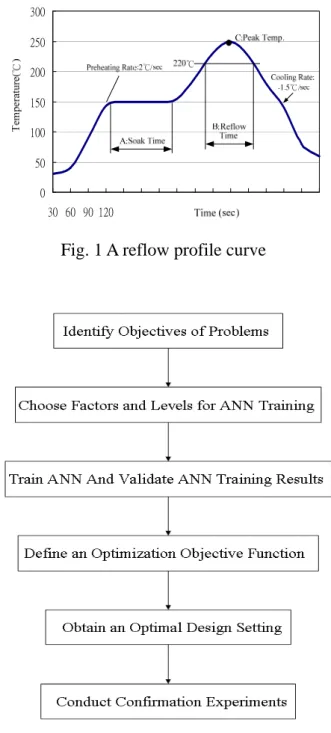
Reflow profiling
A reflow profile (i.e., a thermal profile) is one of the key variables having significant influences on the product qualities and the yield. Normally, there are four process zones for the conventional reflow procedure: the preheating cycle, the thermal soak stage, the reflow cycle and the cooling phase.
of the experiments.
Experimental procedures and test results
Experimental design62 spherical solder balls with 0.45mm in the diameter are required to attach onto a PCB surface. Since the parameter setting of a reflow profiling relates to solder properties, product specifications and the equipment performance, etc., the soak time, the reflow time and the peak temperature were selected as three controllable parameters according to the recommendation from an operation manual of the Der Pan Electric Mechanical Industrial Co.
Figure 1 illustrates a typical reflow profiling applied to the reflow soldering process for the PCB fabrications. In Figure 1, the preheating rate and the cooling rate have been fixed to 2 oC/sec and -1.5 oC/sec, respectively. Furthermore, the experiments were conducted based on an orthogonal array L9 table arrangement with three controllable 3-level factors and one
response variable. Table I lists the three controlled factors including the soak time (i.e., the factor “A” in sec) with solder temperature of 150 oC, the reflow time (the factor “B” in sec) with 220 oC of solder temperature and the peak temperature (the factor “C” in oC).
The selected response variable is the average of the 62 measured ball shear forces after the reflow soldering process. Therefore, it is desirable to have a maximum value.
Ball shear tests of solder spheres
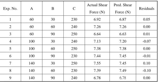
The ball shear test was performed according to the Joint Electron Device Engineering Council (JEDEC) Test Method B117 (JEDEC, 2000) using a Instron 5548 machine with a cross-head speed of 300 μm/s at a shear height of 60μm above the module surface. The recorded amplitude of solder sphere shear forces is an average value of the 62 measured points on the PCB surface by applying forces in a horizontal direction. The measured results are listed in Table II.
Optimization processes
Figure 2 gives the processes of finding an optimal setting for the reflow soldering process. Details of each step are shown at the following subsections.
Identify the objective of the problem
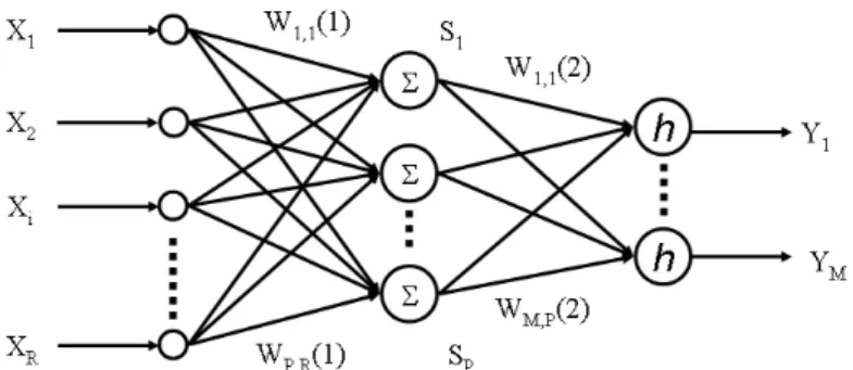
The objective is to identify an optimal setting to maximize an average shear force of solder balls as well as minimize the manufacturing cycle time. An integrated algorithm with an ANN and the SQP method is proposed. An ANN is served as an effective modeling tool to map the relationship between the inputs and the outputs. The ANN learns to approximate the functions through a training process. During the training stage, the training data are presented to an ANN and the network continues to adjust its weights and biases to match the known targets until a performance index reaches a preset threshold value. A multi-layer-feed-forward neural network (MLFN) is selected for its simple architecture, flexibility, and being capable of approximating any complicated functions with a finite number of discontinuities by just adding additional neurons or more hidden layers. A typical MLFN architecture with R input neurons, P hidden neurons, and M output neurons is shown in Figure 3. In Figure 3, Wi,j(k) is the k-th set of weights and biases connecting an ANN
to a range of [-1,1] by a tan-sigmoid function; h is a linear transfer function that transfer the network values from the previous layer to any values (MathWorks, 1997).
Choose factors and levels for ANN training
Referring to an operation manual of the Der Pan Electric Mechanical Industrial Co., we have selected three controllable factors, which are the soak time, the reflow time and the peak temperature. Each factor has three levels to cover the domain of interest. An average shear force of solder balls is the selected output. In Figure 4, the soak time, the reflow time and the peak temperature are fed into the three input neurons and then the output neuron gives the values of the average shear force.
Train ANN and validate ANN training results
Nine sets of data conforming to Taguchi L9 design have been procured and the inputs
data have been scaled between -1 and 1 to improve the training efficiency (MathWorks, 1997). During the training, one of the known problems is called overfitting. An overfitting trained ANN has very poor generalization capability when new data are presented to it. To improve the generalization, a regularization scheme is proposed by modifying a performance index, which is normally defined as a mean square error shown as follows,
∑
∑
= = − = = N i i i N i i T Y N E N MSE 1 2 1 2 ) ( 1 1 (1)where N is the total number of data points; Ti , Yi , and Ei are the target values, the ANN
outputs during training, and the differences of Tiand Yi, respectively. By adding the weights
and the biases into a performance index shown on the equation (1), ANN generalization capability can be greatly improved. A modified performance index is written in the following form, MSW MSE MSEmod =β∗ +(1−β)∗ (2) MSW is defined as follows, β
where is a performance ratio and
∑
= n w MSW 2 = j j n 1 1 (3)where n is the total numbers of weights and biases; wj represents the weights and the biases.
tion and obtain an optimum setting
During the training, the values feeding into the ANN input neurons have been limited to Applying this new performance index will force the network to have smaller values of weights and biases, the network response will be smoother and less likely to overfit. Nevertheless, it is very difficult to determine an optimal regularization parameter. Hence, Mackay et al. (Mackay, 1992; Foresse and Hagan, 1997) performed Bayesian regularization to automate the selection of the optimal regularization parameter. After completing the training, two additional data that have not been seen by the ANN are utilized to validate the training results. If the validation is satisfactory, the ANN will be used to find an optimal parameter setting stated in the following section.
the domain of interest; thus, once the ANN has been properly trained, it gives the reasonable outp
subject to
(4)
where x is the vector of design p
uts when presented with the inputs falling within the training range even the data have never been seen by the network. Namely, the trained ANN performs well on interpolation. On the other hand, if the data presented to the ANN is outside the region of training, generalization capability of the ANN degrades, i.e. the ANN does poorly on extrapolation. Hence, a feasible optimal solution, which reaches a maximized average shear force, shall be constrained in the domain that has been used to train the ANN. For this type of constrained optimization cases, a general approach is to transform the problem into an easier sub-problem that can be solved and used as the basis of an iterative process. A general problem description is stated as follows (Fletcher, 1981)
) (x f n x∈ℜ min u l e e i x x x m m i m i x C ≤ ≤ + = = = , , 1 , , 1 0 ) ( L L i x C ( )≤ 0
arameters, x={x1,x2,L,xn}, f(x) is the objective function that yields a scalar value; the vector function Ci(x) gives the equality and inequality constraints
of x, xu is the u
(5)
The first equation in the equation (5) describes a canceling between the objective function and the gradients of the active constraints at the solution point, x*. To cancel the grad
values evaluated at x; xl is the lower bound pper bound, and me is the number
of the equality constraints. If the Kuhn-Tucker (KT) equations are applied, the equation (4) can be restated as C x f( ) i * * +
∑
λ ⋅∇ m m i m i x C x e i e i m i i , , 1 0 , , 1 0 ) ( 0 ) ( * * 1 * L L + = ≥ = = ∇ = = λients, Lagrange multipliers (λi,i=1,L,m) are used to balance the deviations in magnitude of the objective function and the constraints gradients. Since only active constraints are included in the canceling operation, the constraints that are not active must not be included in this operation and so are given Lagrange multipliers equal to zero.
The solution of the KT equations is the basis of many nonlinear programming algorithms, which attempt to solve the Lagrange multipliers directly. These methods are referred to as the SQP methods since a Quadratic Program (QP) sub-problem is solved at each major iteration. An overview of SQP can be found in Fletcher (Fletcher, 1981). During the optimization, the trained ANN provides the function values to the SQP algorithm.
average shear forces of solder balls as well as minimize the manufacturing cycle time, the objective function, f(x), can be defined as follows (Myers and Montgomery, 2002),
D x f F F F SF D − − = S S S min max min − = ) ( (6)
where the SFmax an
data for the average shear force. “D” is a desirability function (Myers and Montgomery,
required to reassure the ANN training quality and validate ation runs of the optimal setting yield good results, the prop
ental factors and the factor levels, Table 2 shows the experimental results based on the
e ANN has been trained by the e errors between the experimental data and the ANN training outputs defin
ental data and the ANN predicted values, one
e adequacy of an ANN model shall be inspected to confirm that the model has xperimental data before the ANN model can be
ate of the d the SFmin are the maximum and the minimum values of the experimental
2002), and the objective is to choose an optimal setting to maximize the desirability function “D” and minimize the cycle time.
Conduct confirmation experiments
Confirmation experiments are the optimal setting. Hence, if confirm
osed algorithm is validated.
Results and discussion
As Table 1 gives the experim
orthogonal array L9 design.
ANN training results
Table 3 is the results of the average shear force after th experimental data. Th
ed as the residuals are also shown in the table.
Furthermore, by investigating the correlation coefficients, R2, which measures the strength of a linear relationship between the experim
obtain the value of R2 to be 0.984 after the ANN training. There are about 98.4% of all of the variance in the experimental data can be accounted for by the predicted outputs of the ANN.
ANN model adequacy check
Th
extracted all relevant information from the e
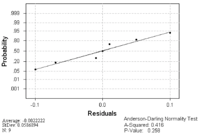
utilized by the SQP algorithm for finding an optimal setting. The primary diagnostic tool is the residual analysis (Montgomery, 1997). The residuals are defined as the differences between the actual and predicted values for each point in the design. The residual results for the shear forces are listed in Table III. If a model is adequate, the distribution of residuals should be normally distributed (Montgomery, 1997). Minitab® (Minitab, 2000) program is used to perform the normality test. For the normality test, the hypotheses are listed as follows, 1. Null hypothesis: the residual data follows a normal distribution
2. Alternative hypothesis: the residual data does not follow a normal distribution
In Figure 5, the vertical axis has a probability scale and the horizontal axis with a data scale. A least-square line is then fitted to the plotted points. The line forms an estim
cumulative distribution function for the population from which data are drawn.
1997
ts to the reflow soldering process and the results are shown in Table 4 after remo
d model is significant and there is only a 0.55% chance that the “Model F value” coul
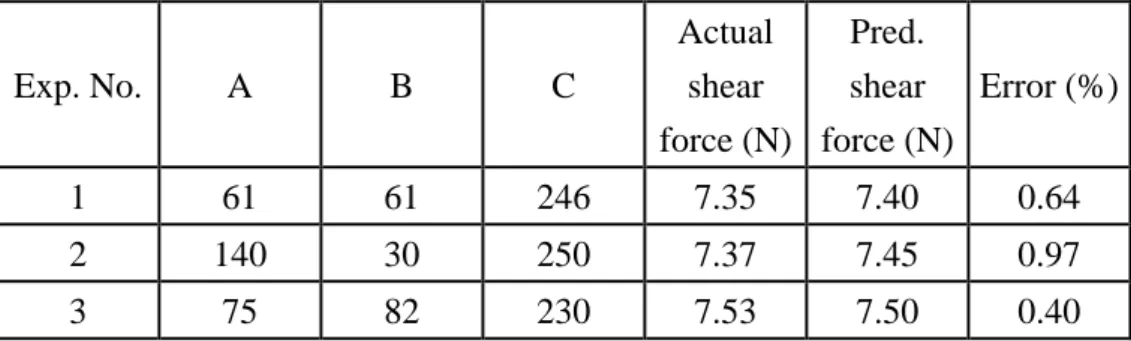
. 1 of Table 5) is conducted with soak time of 61 seconds, C. The second confirmation run (No.
). In view of the fact that the “P-value” shown in Figure 5 is 0.258, which are larger than 0.05, the residuals follow a normal distribution; hence, the ANN predictive model is adequacy and extracts all available information from the experimental data. The rests of information defined as residuals can be considered as errors from performing the experiments.
ANOVA results
The analysis of variance (ANOVA) was conducted to identify the factors that have significant impac
ving any insignificant terms. A “Model F value” is calculated from a model mean square divided by a residual mean square. It is a test of comparing a model variance with a residual variance. If the variances are close to the same, the ratio will be close to one and it is less likely that any of the factors have a significant effect on the response. As for a “Model P value”, if the “Model P value” is very small (less than 0.05) then the terms in the model have a significant effect on the response (Montgomery, 1997). Similarly, an “F value” on any individual factor terms is calculated from a term mean square divided by a residual mean square. It is a test that compares a term variance with a residual variance. If the variances are close to the same, the ratio will be close to one and it is less likely that the term has a significant effect on the response. Furthermore, if a “P value” of any model terms is very small (less than 0.05), the individual terms in the model have a significant effect on the response.
In Table IV, a “Model F value” of 42.46 with a “Model P value” of 0.0055 implies that the selecte
d occur due to the noise. The “P value” for the model term “B” (the reflow time in sec) is 0.0162 and 0.0087 for the model term “B2” indicating that both the model terms “B” and “B2” are significant. There is only one interaction term “BC” having significant influence on the average shear force. In addition, a “P value” for the model term “C2” is 0.033, which is less than 0.05, signifying that the model term “C2” is also significant. According to the hierarchy principle in model-building (Montgomery, 1997), the model term “C” (the peak temperature in oC) shall be also included in the regression model even the “P value” of the model term “C” is more than 0.05.
Confirmation tests for the ANN and an optimal setting
The first confirmation run (No
reflow time of 61 seconds and peak temperature of 246 O
2 of Table 5) is performed with soak rime of 140 seconds, reflow time of 30 seconds and peak temperature of 250 OC. Finally, an optimal setting (No. 3 of Table 5), soak rime of 75 seconds, reflow time of 82 seconds and peak temperature of 230 OC, is identified from the ANN predictive model and the SQP method by maximizing the desirability function “D” in the equation (6) and minimize the cycle time. With this optimal setting, one can get 7.53 N of the average shear force with a desirability function value of 0.98 according to the equation (6). By comparing the optimal setting with an average shear force of 7.53 N to the best shear force results of 7.55 N in a L9 orthogonal array table shown in No. 7 run of Table 2, the
This study investigated the ing process using a hybrid
an be utilized successfully to predict the shear force under different
Conclusions and discussion
optimization of the reflow solder
method that combines the ANN and the SQP method. Nine experimental runs based on the orthogonal arrays table were performed to reduce the number of experiments. The average sustained shear force of solder spheres is adopted as a quality target. According to the experimental data and the analysis of variance (ANOVA), the results are summarized as follows.
1. The ANN c
reflow soldering conditions after being properly trained.
2. In order to achieve a maximum shear force, the optimal parameter settings for the reflow soldering process is with soak time of 75 sec, reflow time of 82 sec and 3. This study provides an algorithm that integrates a black-box modeling approach (i.e.,
the ANN predictive model) and the SQP method to resolve an optimization problem. This algorithm offered an effective and systematic way to identify an optimal setting of the reflow soldering process.
References
Bigas, M. and Cabruja, E. (2006) “Characterisation of electroplated Sn/Ag solder bumps”, Microelectronics Journal, Vol 37 No 3, pp. 308–316.
Choon, T. K and Corpuz (Billie), V. G.. (1999) “High frequency wire bonding for PBGA package, a process optimisation approach”, Microelectronics International, Vol. 16, No 3, pp. 22 – 35.
Der Pan Electric Mechanical Industrial Co. (2005), Equipment Operation Manual: Model: TSK-8000.
Fletcher, R. (1981), Practical Methods of Optimizations, Vol. 1, Unconstrained Optimization and Vol. 2, Constrained Optimization, John Wiley & Sons Inc., New York.
Foresse, F.D. and Hagan, M.T. (1997), “Gauss-Newton approximation to Bayesian regularization”, Proceeding of the 1997 International Joint Conference on Neural Networks, pp. 1930-1935.
Lee, N.C. (1999) “Optimizing the reflow profile via defect mechanism analysis”, Soldering and Surface Mount Technology, Vol 11 No 1, pp. 13-20.
Mackay, D.J.C. (1992), “Bayesian interpolation”, Neural Computation, Vol 3, pp. 415-447
MathWorks, Inc., (1997), 24 Prime Park Way, Natick, MA 01760-1500, USA. Neural Network Toolbox User’s Guide Version. 3.0
Minitab Inc., (2000) Quality Plaza, 1829 Pine Hall Road, State College, PA 16801-3008, USA.
Montgomery, D. C. (1997), Design and Analysis of Experiments, Fourth Edition, John Wiley & Sons, Inc., New York, pp. 101-245.
Myers, R. H. and Montgomery, D. C. (2002), Response Surface Methodology, 2nd Edition, John Wiley & Sons Inc., New York.
Salam, B., Virseda, C., Da, H., Ekere, N. N., and Durairaj, R. (2004) “Reflow profile study of the Sn-Ag-Cu solder”, Soldering and Surface Mount Technology, Vol 16 No 1 , pp. 27-34.
Skidmore, T. and Waiters, K. (2000) “Optimizing solder joint quality-lead free”, Circuits Assembly, pp. 17-22.
Suganuna, H. and Tamanaha, A. (2001) “Reflow Technology”, SMT Magazine, pp. 65-70.
Taguchi, G.. (1991), Introduction to Quality Engineering: Designing Quality into Products and Processes, 2nd Edition, Asian Productivity Organization, Japan.
Yang, F. H. and Lee, K. Y. (2005) “Application of a design of experiments approach to the reliability of a PBGA package”, Soldering and Surface Mount Technology, Vol 17 No 3, pp. 43-53.
0 50 100 150 200 250 300 30 60 90 120
Fig. 1 A reflow profile curve
Fig. 3. A typical MLFN architecture with R input neurons, P hidden neurons, and M output neurons
Fig. 4. Architecture of the MLFN with one output neuron of the average shear forces
Reflow time
Σ Σ
Σ h Averaged shear force
Σ Σ Peak temperature Soak time Reflow time Σ Σ
Σ h Averaged shear force
Σ Σ Peak temperature
Table 1 Experimental factors and factor levels
Experimental factors Levels of
experimental
factors A/sec B/sec C/ oC
1 60 30 230 2 100 60 240 3 140 90 250 L9 A B C Shear forces (N) 1 60 30 230 6.92 2 60 60 240 7.26 3 60 90 250 6.64 4 100 30 240 7.13 5 100 60 250 7.38 6 100 90 230 7.44 7 140 30 250 7.55 8 140 60 230 7.39 9 140 90 240 6.78
Table 2 Orthogonal array L9 (34) of the experimental runs and results
Table 3 Residual results shear forces
Table 4 ANOVA results for shear forces
Source Sum of squares Degree of
freedom Mean square F value P value Model 0.8035 5 0.16069 42.46 0.0055 B 0.0913 1 0.09127 24.12 0.0162 C 0.0054 1 0.00540 1.43 0.3181 B2 0.1422 1 0.14222 37.58 0.0087 C2 0.0534 1 0.05336 14.10 0.0330 BC 0.5112 1 0.51123 135.09 0.0014 Residual 0.0114 3 0.00378 - - Total 0.8148 8 - - -
Table 5 Confirmation runs with one optimal setting with maximizing shear f
97 年度
明新科技大學 97 年度 研究計畫執行成果自評表
計 畫 類 別 : □任務導向計畫 □整合型計畫;
個人計畫 所 屬 院 ( 部 ) :;
工學院 □管理學院 □服務學院 □通識教育部 執 行 系 別 : 機械系 計 畫 主 持 人 : 謝傑任博士 職 稱:副教授 計 畫 名 稱 : 利用類神經系統於 BGA 封裝迴焊製程的最佳條件研究 計 畫 編 號 : MUST-97 機械-03 計 畫 執 行 時 間 : 97 年 1 月 1 日 至 97 年 9 月 30 日 教 學 方 面 1.對於改進教學成果方面之具體成效: 使學生了解封裝之製程與相關業界規範。並教導研究生如何利用Matlab程式語言 解決最佳化之相關問題。 2.對於提昇學生論文/專題研究能力之具體成效: 研究生學習Matlab之人機介面程式與利用實驗計畫法分析資料 3.其他方面之具體成效:利用類似之方法與研究手段,已完成了二篇SCI期刊論 文計
畫
執
行
成
效
學 術 研 究 方 面 1.該計畫是否有衍生出其他計畫案 □是;
否 計畫名稱: 2.該計畫是否有產生論文並發表 □已發表 □預定投稿/審查中 □否發表期刊(研討會)名稱:Expert Systems with Applications