A Novel Approach to Supervised Hyperspectral Image Classification

A Novel Approach to Supervised Hyperspectral Image Classification

Yang-Lang Chang

¹

Chin-Chuan Han

²

Kuo-Chin Fan

³

K .S. Chen

⁴

ABSTRACT

This paper presents a new supervised classification technique for hyperspectral imagery, which consists of two algorithms, referred to as greedy modular eigenspace (GME) and positive Boolean function (PBF). The GME method is designed to extract features by a simple and efficient GME feature module. The GME makes use of the data correlation matrix to reorder spectral bands from which a group of feature eigenspaces can be generated to reduce dimensionality. It can be implemented as a feature extractor to generate a particular feature eigenspace for each of the material classes present in hyperspectral data. The residual reconstruction errors (RRE) are then calculated by projecting the samples into different individual GME-generated modular eigenspaces.

The PBF is further developed for classification. It is a stack filter built by using the binary RRE as classifier parameters for supervised training. It implements the minimum classification error (MCE) as a criterion so as to improve classification performance. It utilizes the positive and negative sample learning ability of the MCE criteria to improve classification accuracy. The performance of the proposed method is evaluated by MODIS/ASTER airborne simulator (MASTER) images for land cover classification during the Pacrim II campaign. Experimental results demonstrate that the GME feature extractor suits the nonlinear PBF-based multi-class classifier well for classification preprocessing. The proposed approach is not only an effective method for land cover classification in earth remote sensing but also dramatically improves the eigen-decomposition computational complexity compared to the conventional principal components analysis (PCA).

Key Words: principal components analysis (PCA), hyperspectral supervised classification,

greedy modular eigenspaces (GME), positive Boolean function (PBF), stack filter.

Received Date: Nov. 11, 2003 Revised Date: July 25, 2004 Accepted Date: July 27, 2004

1.Associate Professor, Department of Information Management, National Taipei College of Business

2.Associate Professor, Department of Computer Science and Information Engineering, National United University

3.Professor, Institute of Computer Science and Information Engineering, National Central University

4.Professor, Center for Space and Remote Sensing Research, National Central University

1. INTRODUCTION

With the evolution of remote sensing technology, an increasing number of spectral bands become available. Data can be collected in a few multispectral bands to as many as several hundreds hyperspectral bands, even thousands of ultraspectral bands.

A lot of attention has been focused on the developing of high-dimensional classification devoted to earth remote sensing. The increment of such high-dimensional data greatly enhances the information content, but provides a challenge to the current techniques for analyzing such data. This improved spectral resolution also comes at a price, known as the curse of dimensionality. That term is used by the statistical community to describe the difficulties associated with the feasibility of distribution estimation in high-dimensional data sets. One of most common issues in hyperspectral classification is how to achieve the best class separability without the restriction of limited number of training samples (Jimenez and Landgrebe, 1999; Kumar et al., 2001). Numerous

techniques have been developed for feature extraction to reduce dimensionality without loss of class separability. Most of them focus on the estimation of statistics at full dimensionality to extract classification features. For example, the most widely used conventional principal components analysis (PCA) assumes the covariances of different classes are equal, i.e. a common covariance pool (matrix) is used, and the potential differences between class covariance are not utilized. The PCA reorganizes the data coordinates in accordance with data variances so that features are extracted based on the magnitudes of their corresponding eigenvalues (Richards and Jia, 1999). Fisher discriminant analysis uses the between-class and within-class variances to extract desired features and to reduce dimensionality (Duda and Hart, 1973). Another example is the orthogonal subspace projection (OSP) recently developed by Harsanyi and Chang (1994). OSP projects all undesired pixels into a space orthogonal to the space generated by the desired pixels to achieve dimensionality reduction.

Figure 1. Data flow of the proposed GME/PBF-based multi-class classification scheme.

This paper presents a new approach to achieve dimensionality reduction while increasing classification accuracy. It is comprised of two algorithms, greedy modular eigenspace (GME) and positive Boolean function (PBF). The GME based on a correlation matrix (the second order statistic) is developed by grouping highly correlated bands into a small set of bands. The GME overcomes the dependency on the global statistics as much as possible, while preserving the inherent separability of the different classes. Most classifiers seek only one set of features that discriminates all classes simultaneously. This not only requires a large number of features, but also increases the complexity of the potential decision boundary. This paper will show that the proposed GME/PBF method solves this problem and improves classification accuracy. The GME provides a very good discrimination among the classes of interest using the idea of modular eigenspaces description which had been proved to have very high recognition rates for the face recognition (Pentland and Moghaddam, 1994).

The approach uses a greedy condensed correlation coefficient matrix reordering transformation to find a set of high correlated GME. It performs a greedy iteration search algorithm which reorders the correlation coefficients in the data correlation matrix row by row and column by column to group highly correlated bands as GME feature eigenspaces that can be further used for feature extraction.

Reordering the bands regardless of the original order of wavelengths and spectrally adjacent bands in high-dimensional data set is an important characteristic of GME. The well-known segment principal components analysis (PCA) technique has a very high accuracy in remote sensing image classification (Jia et al., 1999) and (Richards et al., 1999).

Our proposed GME improves the segment PCA performance by reordering the band order to reproduce a new and efficient GME subspaces from the correlation matrixes.

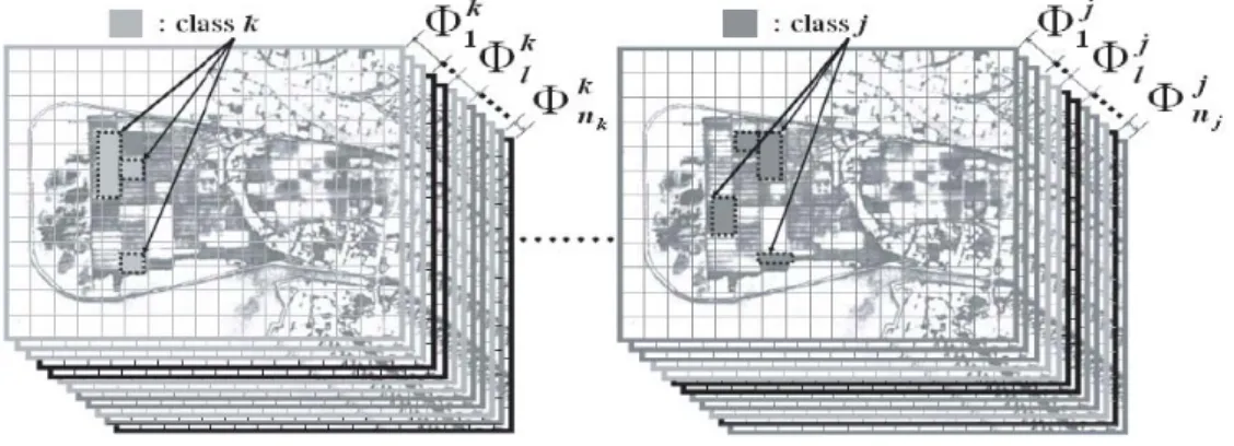
The proposed GME approach divides the whole set of high-dimensional features into several arbitrary number of highly correlated subgroups. It makes good use of these highly corrected band subgroups to speed up the computational time of PCA. Each ground cover type or material class has a distinct set of GME-generated feature eigenspaces. When a set of GME-based feature eigenspaces Φ^k is generated from the training samples, a modular eigenspace projection is next taken to calculate the residual reconstruction error (RRE) vectors e^k for the class ωk. These RRE vectors are then normalized and quantized before being applied to the subsequent PBF-based classifier.

The follow-up PBF is developed to design a multi-class classifier that can take advantage of using the binary RRE as its training samples and can also fully utilize minimum classification error (MCE) (Juang et al., 1997) learning ability as its optimization criterion to explore the special characteristics of GME. The

MCE characteristic can best combine the PBF-based multi-class classifier with the binary RRE generated from GME. Finally, a classification map, Ω, can be obtained by applying the PBF-based multi-class classifier to test samples. Fig. 1 illustrates the flow chart of this GME/PBF-based multi-class classification scheme.

Recently, several hyperspectral data feature extraction and reduction techniques have been developed that are well suited for

application to pairwise classifier architectures to enhance classification accuracy. Jimenez et al. (1999) proposed a projection pursuit method utilizing a projection index function to select potential interesting projections from the local optimization-over-projection directions of the index (Bhattacharyya distance between two classes) of performance. A best-bases feature extraction algorithm developed by Kumar et al.(2001) used an extended local discriminant bases technique to reduce the feature spaces.

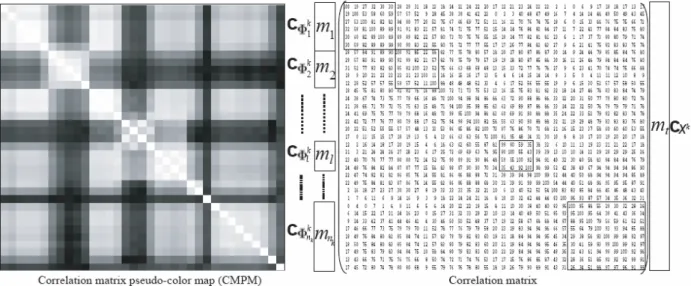
Figure 2. An example illustrates a CMPM with different gray levels and its corresponding correlation matrix with different correlation coefficients in percentage (White = 100; black = 0) for the class ωk. Note that four squares with fine black borders represent the highly correlated modular subspaces which have higher correlation coefficient compared with their neighborhood.

Both of them used pairwise classifiers to divide multi-class problems into a set of two-class problems. Our proposed GME/PBF-based classifier performs multi-class classification which was previously proposed in Refs. (Han and Tsai, 2001, and Han, 2002) to enhance the precision of image

classification significantly by exploring the capabilities of multi-class classifiers rather than pairwise classifiers. The main characteristic of a PBF-based multi-class classification scheme is its nonlinear discrete properties. It makes use of MCE criteria (Juang et al., 1997) to apply both positive and negative

samples of the binary RRE as training samples for the PBF-based multi-class classifier. The features of GME are very well suited to the PBF-based multi-class classification properties compared to traditional feature extraction.

These facts will be best demonstrated in experimental results.

The rest of this paper is organized as follows.

In Section 2, the proposed GME/PBF-based multi-class classifier is described in detail. In Section 3, a set of experiments is conducted to demonstrate the feasibility and utility of the proposed approach. Finally, in Section 4, several conclusions are presented.

2. METHODOLOGY

A visual scheme to display the magnitude of correlation matrix for emphasizing the second-order statistics of high-dimensional data was proposed by Lee and Landgrebe (1993). Shown in Fig. 2 is a correlation matrix pseudo-color map (CMPM) in which the gray scale is used to represent the magnitude of its corresponding correlation matrix. It is also equal to a modular subspace set Φ

^k

. Different material classes have different value sequences of correlation matrices. It can be treated as the special sequence codes for feature extractions. We define a correlation submatrix

cΦ1^k

(m

l ×ml

) which belongs to the

l^th

modular subspace Φ

^kl

of a complete set Φ

^k = (Φ^k1,...Φ^kl,...Φ^nkk

) for a

class ωk, where ml and nk represent, respectively, the number of bands (feature spaces) in modular subspace Φ

^kl

, and the total number of modular subspaces for a complete set Φ

^k

, i.e. l

^∈

{1,...,nk} as shown in Fig. 2. The original correlation matrix c

^Xk

(m

t×mt

) is decomposed into nk correlation submatrices c

^Φk1(m¹×m¹),..c^Φkl(m^l×m^l),...c^Φnkk(m^nk×m^nk)

to build a GME set Φ

^k

for the class ωk.

There are mt! (the factorial of mt) possible combinations to construct one complete set exactly. The

mt represents the total number of original

bands, ∑ ,

=

=

^nk

1 l

l

t m

m (1) where ml represents the l^th feature subspace of a complete set for a class ωk.

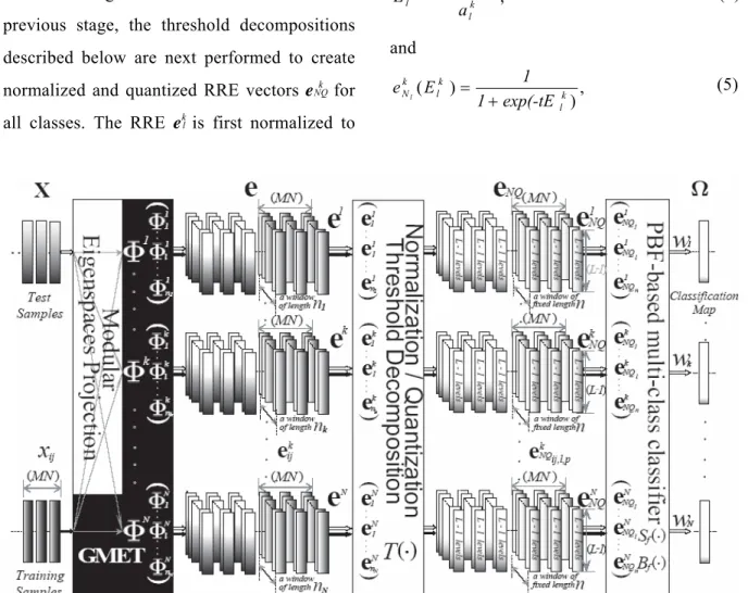
Referring to Fig. 1, there are four stages to implementing our proposed GME/PBF-based multi-class classification scheme. 1) A GME transformation algorithm is applied to achieve dimensionality reduction and feature extraction.

2) The second stage is a modular eigenspace projection similarity measure also known as distance decomposition. 3) The third stage is a threshold decomposition which normalizes and quantizes the RRE. 4) Finally, a PBF-based multi-class classification is performed.

2.1. Greedy Modular Eigenspaces

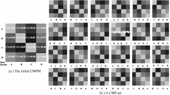
We firstly define a complete modular subspace (CMS) set which is composed of all possible combinations of the CMPM. The

original correlation matrix c^Xk (mt×mt) is decomposed into n^k correlation submatrices c^Φk1

(m^1×m¹⁾,...c^Φkl(m^l×m^l),...c^Φnkk(m^nk×m^nk) to build a CMPM for the class ωk. There are mt! different kinds of CMPMs in a CMS set as shown in Fig.

3. Each different CMPM is associated with a

unique sequence of band order. It needs mt! swapping operations by band order to find a complete and exhaustive CMS set. In Fig. 4, a visual interpretation is introduced to highlight the relations between swapping and rotating operations in terms of band order.

Figure 3. (a.) The initial CMPM for four original bands (A, B, C and D), mt = 4, is applied to the exhaustive swapping operations by band order. (b.) An example shows a CMS set which is composed of 24 (mt!

= 4!) possible CMPMs. The CMPM with a dotted-line square is the optimal CMPM in a CMS set.

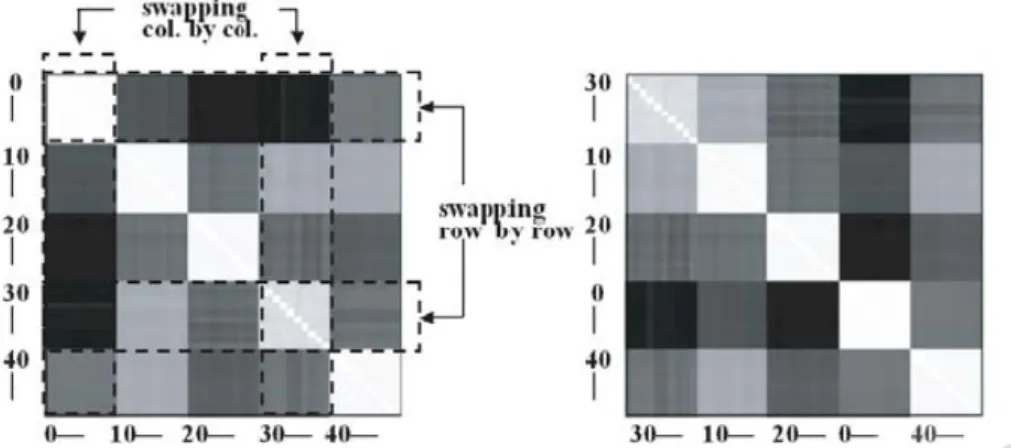
Figure 4.The rotation operation between the Block K and Block 2 is performed by swapping their horizontal and vertical correlation coefficient lists row by row and column by column. Note that a pair of blocks (squares) switched by this swapping operation in terms of band order should have the same size of any length along the diagonal of correlation matrices. The Fixed Blk 1 and Fixed Blk 2 will rotate 90 degrees.

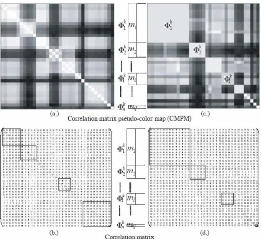
Figure 5. (a.) and (b.) The original CMPM and its corresponding correlation matrix for class k. (c.) and (d.) The GME set Φ^kfor class ωk and its corresponding correlation matrix after greedy modular subspaces transformation.

There is one optimal CMPM in a CMS set as shown in Fig. 3. This optimal CMPM is defined as a specific CMPM which is composed of a set of modular subspaces Φ_l^k, l

∈{1,...l,...nk} and Φ_l^k∈ Φ^k. It has the highest correlated relations inside each individual modular subspace Φ_l^k. It tempts to reach the condition that the high correlated blocks (with high correlation coefficient values) are put together adjacently, as near as possible, to construct the optimal modular subspace set in the diagonal of CMPM. It is too expensive to make an exhaustive computation for a large

amount of mt to find an optimal CMPM in a CMS set. In order to overcome this drawback, we develop a fast searching algorithm to construct an alternative greedy CMPM (modular subspace) instead of the optimal CMPM. This new greedy CMPM is defined as a GME feature module set. It can not only reduce the redundant operations in finding the greedy CMPM but also provides an efficient method to construct GME sets.

In this paper, we propose a GME set

Φ^k

which is composed of a group of

modular eigenspaces. Each modular

eigenspace Φ

^k

includes a set of highly correlated bands regardless of the original order of wavelengths. There are some

merits to this scheme. 1) It reduces the number of bands in each GME set to speed up the eigen-decomposition computation compared with conventional PCA. 2) A highly correlated GME makes PCA work more efficiently due to the redundancy reduction property of PCA. 3) The GME tends to equalize all the bands in a subgroup with highly correlated variances to avoid potential bias problems that may occur in conventional PCA (Jia and Richards, 1999). 4) Different classes are best distinguished by different GME abundant feature sets.

We define a correlation submatrix c^Φkl(m^l

×m^l) which belongs to the l^th modular eigenspace Φ^kl of a GME Φ^k = (Φ^k1,...Φ^kl,...Φ^nkk) for a class ωk, where ml and nk represent, respectively, the number of bands in modular eigenspaces Φ^kl, and the total number of modular eigenspaces of a GME set Φ^k, i.e. l ∈ {1,...,nk } as shown in Fig. 5. The original correlation matrix c^Xk(m^t×m^t), where mt is the total number of original bands, is decomposed into nk correlation submatrices c^Φ1k(m^1×m¹⁾,...c^Φkl

(m^l×m^l),...c^Φnkk(m^nk×m^nk)to build a GME set Φ^k for the class ωk. There are mt! possible combinations to construct a candidate GME set as a CMS set dose. That is to say, it takes mt! operations to compose mt! different sets of the correlation submatrices associated with different sequences of band order. Only one of them can be chosen as the GME set.

It is computationally expensive to make an exhaustive search to construct a GME set if mt is a large number. In this paper, we propose a fast greedy band reordering algorithm, called greedy modular eigenspace transformation (GMET), based on the assumption that highly correlated bands often appear adjacent to each other in hyperspectral data (Richards and Jia, 1999). In this algorithm, the absolute value of every correlation coefficient ci,j in the correlation matrix c^Xk is compared to a threshold value t^c (0 ≤ t^c≤ 1). Those adjacent correlation coefficient ci,j that are larger than the threshold value t^c are used to construct a modular eigenspace Φ^kin an iterative mode. A greedy searching iteration is initially carried out at c^0,0 ∈ c^Xk(m^t x m^t) for a class ωk to condense a GME set. Each ci,j is assigned an attribute during a GMET. If the attribute of a c^i,j j is set as available, it means this ci,j has not been assigned to any modular eigenspace Φ^k. If a ci,j is assigned to a modular eigenspace Φ^kl, the attribute of this ci,j is set to used. All attributes of the original correlation matrix c^Xk are first set as available. The proposed GMET algorithm is as follows:

Step 1. Initialization: A new modular eigenspace Φ^kl ∈ Φ^k for a class ωk is initialized by a new correlation coefficient c^d,d, where c^d,d and d are defined as the first available element and its subindex in the diagonal list [c^0,0,...c^m_t^−1,m_t⁻¹] of the correlation matrix c^Xkrespectively. This diagonal coefficient

c^d,d is set to used and then assigned as the current c^i,j , i.e. the only one activated at the current time. Then, go to step 2. Note that this GMET algorithm is terminated if the last diagonalcoefficient c^d,d is already set to used and the last subgroup Φnk^k of the GME has been obtained for class ωk.

Step 2. If the column subindex j of the current c^i,j has reached the last column (i.e. j = m^t − 1) in the correlation matrix, then a new modular eigenspace Φ^kl is constructed with all used correlation coefficients c^i,j ∈ Φ ^kl , these used coefficients c^i,j are then removed from the correlation matrix, and the algorithm goes to step 1 for another round to find a new modular eigenspace. Otherwise, it goes to step 3.

Step 3. GMET moves the current c^i,j to the next adjacent column c^i,j+1 which will act as the current c^i,j, i.e. c^i,j →c^i,j+1. If the

current c^i,j is available and its value is larger than t^c, then go to step 4. Otherwise, go to step 2.

Step 4. If j≠d, swap c^∗ ,j with c^∗ ,d and c j,∗ with cd, ∗ respectively, where the asterisk symbol ”*” indicates any row or column subindex in the correlation matrix.

Fig. 4 and Fig. 6 shows a graphical mechanism of this swapping operation.

The attributes of c^{d, ∗} and c^{∗ ,d} are then marked used. Then let c^i↔d,d and c^d,i↔d∈Φ^kl , where i ↔ d means including all coefficients between subindex i and subindex d. Go to step 2.

Eventually, a GME set, Φ^k = (Φ^k1,...Φ^kl,...Φ^nkk), is composed for ground cover class ωk . For convenience, we sort these modular eigenspaces according to the number of their feature bands, i.e. the number of feature spaces m¹,...m^l,...m^nkk, in descending order.

Figure 6. The original CMPM (White=1 or -1; black=0) and the CMPM after swapping band Nos.0-9 and 30-39.

Figure 7. GME sets for the six ground cover types used in the experiment. Each of them can be treated as a unique feature for a distinguishable class.

Figure 8. The GME sets for different ground cover classes ωk,...ωj. A GME set Φ^kis composed of a group of modular eigenspaces (Φk1,...Φkl,...Φ knk).

Each square (ml ×ml) is filled with an average value of all correlation coefficients inside its correlation submatrix cΦ^kl(ml×ml).

Fig. 5 illustrates the original CMPM and the reordered one after a GMET. Each ground cover type or material class has its uniquely ordered GME set. For instance, in our experiment, six ground cover types were transformed into six different GME sets as shown in Fig. 7.

In this visualization scheme, we can build a GME efficiently and bypass the redundant procedures of rearranging the band order from the original hyperspectral data sets. Moreover, the GMET algorithm can tremendously reduce the eigen-decomposition computation compared to the feature extraction of conventional PCA. The computational complexity for conventional PCA is on the order of O(m^t2) and it is O(Σ^i=1nk m²i) for GME

(Jia and Richards, 1999). It makes good use of these highly corrected band subgroups to speed up the computational time while it compared to the PCA computation of the whole set of bands.

An example in which the GMET was applied to real hyperspectral data is shown in Fig. 8.

After finding the highly correlated GME sets Φ^k for all classes, k ∈{1,...,N}, the eigenspace projections are executed.

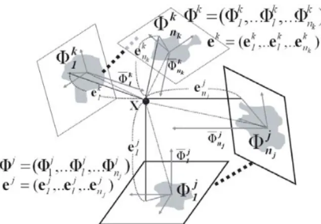
Figure 9. The RRE for classes ωj and ωk in the hyperplane.

2.2. Distance Measures: Greedy Modular Eigenspace Projection

The GME can distinguish different classes well by their individual highly correlated features of modular eigenspace. It can make use of the PCA, also known as the Karhunen-Loe´ve Transform (Han and Tsai, 2001), to extract the most significant information as a similarity measure from each GMET-generated eigenspace while removing redundancy in the spectral domain. Let us assume Φ^kl , which is the l^thmodular eigenspace of the GME set Φ^k

for class ωk, has ml feature bands as shown in Fig. 5. The basis functions in a PCA are obtained by solving the eigenvalue problem

Λ

^kl= φ^klTΣ^klφ^kl , (2) where Σ is the covariance matrix of Φ^kl, φ^kl is the eigenvector matrix of Σ, and Λ is the corresponding diagonal matrix of eigenvalues.

Moghaddam et al. (1995) decomposed the vector space R^ml into two exclusive and complementary subspaces: the principal subspace (W feature spaces) φ^kl = {φ^kli}i=1^W and orthogonal complement subspace φ—_k

l = {φ^kli}i=W+1^ml , where φli^k is the i^th eigenvector of φ^kl. A residual reconstruction error of the modular eigenspace Φ^kl is defined as:

, )

(

2

∑

∑

+ =

=

−

=

= ^W

1 j

2 j m ~

1 W j

2 j k

i x y x y

e ⁱ (3)

where x~

= x - x—

is the mean-normalized vector of sample x. yj is the projected value of sample x by the eigenvector φli^k corresponding with the i^th largest eigenvalue. Here, e^kl (x) represents the distance between the query sample x and the modular eigenspace Φ^kl of the training samples. This GME projection also known as distance decomposition is applied to all modular eigenspaces Φ^kl , l ∈{1,...l,... nk }, to generate an RRE vector e^k =(e^k1,... e^kl ,... enk^k ) for class ωk. The drawing interpretation of the RRE vectors is depicted in Fig. 9. For convenience, we redefine this distance measure, RRE, as an RRE-decomposition (distance decomposition).

2.3. Threshold Decomposition

After defining the RRE vector e^k from the previous stage, the threshold decompositions described below are next performed to create normalized and quantized RRE vectors eNQ^k for all classes. The RRE e^klis first normalized to

the range (0,1) by the nonlinear sigmoid function:

k ,

l k l k k l

l a

µ

E e −

= (4)

and

), )

( _k

l k

l k

N 1 exp(-tE

E 1 e _l

= + (5)

Figure 10. Determination process of GME/PBF-based multi-class classification scheme for supervised hyperspectral image classification.

where µ_l , a^k and t denote the mean and the standard deviation of the RRE e^kl and a threshold value respectively. This new normalized RRE e^Nlk is then uniformly quantized into L−1 levels.

Finally, these normalized distance vectors e^Nk =(e^N1k ,.. e^Nlk ,.. e^Nnkk ) are converted into binary vectors e^NQk =(e^NQl1k ,... e^NQllk ,...e^NQlnkk ), where l

∈ {1,...,L −1}. In Fig. 10, the threshold decomposition function T(·) transforms the

RRE vectors e^k into the binary RRE vectors e^NQk for all classes ωk, where k ∈ {1,...,N}.

2.4. Stack Filter and Positive Boolean Function

The PBF is developed from a stack

filter. Each stack filter corresponding to a

PBF possesses the weak superposition

property (the threshold decomposition)

and the ordering property (the stacking property) (Wendt et al., 1986). The class of stack filters includes many familiar filter types, such as median filter, weighted median filter, order statistic filter and weighted order median filter.

The main function of a stack filter is to remove noise, detect edges, etc. This technology has received considerable interest in communications and signal processing communities. Wendt et al.(1986) defined stack filters as the class of all nonlinear digital filters and pointed out the consonant connections between stack filters and PBF. Maragos (1987) used mathematical morphology to construct a class of morphological filters and their equivalent classes. He also showed that a PBF has exactly one sum-of-product form or one

product-of-sum form produced by morphological operations. Dougherty (1992) defined a basis class of filters satisfying the morphological basis

criteria and applied the erosion operation

as an estimator to find the optimal morphological filter by minimizing the

mean square error. Postaire (1993) et al.

proposed a binary morphological technique to cluster the N-dimensional observations. It is an un-supervised pattern clustering approach based on mathematical morphological operations. Lin and Coyle (1990) developed a generalized stack filter, including all rank order filters, stack filters, and digital morphological filters. They showed that choosing a generalized stack filter is equivalent to massively parallel threshold-crossing decision making when these decisions are consistent with each other.

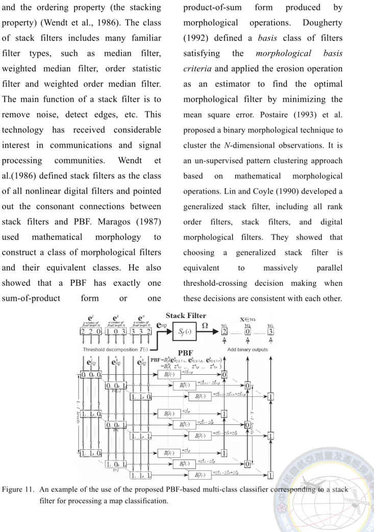
Figure 11. An example of the use of the proposed PBF-based multi-class classifier corresponding to a stack filter for processing a map classification.

In traditional supervised pattern classification, the Bayes decision theory models the classification as a distribution estimation problem. The Bayes theory can be used to solve classification problems, but it requires complete knowledge of probability distributions. In hyperspectral data, obtaining such complete knowledge is generally difficult even in an unsupervised manner. This is because samples used for training and learning may be mixed pixels and do not provide accurate information. Juang et al. (1997) indicated the superiority of MCE method over the distribution estimation method. The goal of MCE training is to be able to correctly discriminate the observations for best classification results rather than to fit the distributions to the data.

An optimal stack filter Sf is originally defined as a filter whose mean absolute error (MAE) between the filter’s output and the desired signals is minimum value. Since it possesses the well-known threshold decomposition and stacking properties, the multi-level MAE value can be decomposed into a summation of absolute errors occurring at each level. Han (2002) proposed an alternative PBF-based multi-class classification scheme based on MCE criteria to resolve multi-class problems. We further apply this MCE version of a PBF-based classification scheme to remote sensing hyperspectral imagery. It has the ability to learn from both

positive and negative samples of the binary RRE generated simultaneously from GME. It can take all competing classes into consideration when searching for the PBF-based classifier parameter. This is very important because we lack complete knowledge of the data distribution particularly in dealing with hyperspectral data. It also makes multi-class classification possible for our proposed method. The proposed binary RRE vector eNQ^k , fully utilizes the special characteristics of MCE criteria. It not only improves the classification accuracy but also overcomes the restriction of a limited number of training samples which is one of the most common problems in hyperspectral classification of remote sensing. In our approach, an optimal stack filter Sf is defined as a filter whose MCE between the output and the desired signals is minimum value. We apply the window of length n to the number of modular eigenspaces Φ^kfor all classes. As an example, Fig. 10 and Fig. 11 show that the windows of fixed length n slides consist of binary RRE eNQ^k, of all classes. They are used as the MCE training parameters for a PBF.

At the supervised training stage, each level of the training samples is assigned to true (1) or false (0). We assume there are N ground cover classes. We extract only the first n elements of eNQ^k, (eNQ1^k ,...eNQn^k ), as a window of fixed length n for all classes, where n ≤nk for all classes ωk and k ∈{1,...,N}, to develop a

PBF-based multi-class classifier. A PBF is exactly one sum-of-product form without any negative components. The classification errors can be calculated from the summation of the absolute errors incurred at each level. The proposed scheme is constructed by minimizing the classification error rate using the training samples. In Fig. 10, we assume there are N classes of training samples. M stands for a fixed number of training samples for each class ωk. MN training samples are projected to N GME sets and then decomposed into MN² binary RRE vectors e^NQk in the GME projection stage and threshold decomposition stage respectively. Let xij and e^NQk _ij represent MN training samples and MN² binary vectors e^NQk of length n respectively, where i ∈{1,...,N}, j ∈ {1,...,M}and k ∈{1,...,N}. Next, the desired values for each occurrence at each level have to be determined for the output of the PBF. The desired value of an occurrence e^NQk _ij can be treated as the error value of sample xij at class ωk. If sample xij belongs to class ωk, it means that no error occurs, i.e. the desired value of e^NQk_ij is 0. Otherwise, it is equal to 1.

⎩⎨

⎧

∉

≠

∈

= =

k ij

k ij ij

k

NQ if i k,x x k, i if e

d ω

ω 1

) 0

( , (6)

According to the PBF criteria (Han, 2002), a Boolean function B^kf (·) is defined as an occurrence e^NQijlpk at level l in a window of fixed length n (the number of Boolean binary variables) for the class ωk as shown in Fig. 11, where l∈{1,...,L−1} and p∈{1,...,n}.

Based on the threshold decomposition property, an occurrence of binary RRE vector e^kNQ_ij as an input of PBF can be decomposed into binary vectors e^NQijlk = (e^NQijl1k ,...e^NQijlpk ,...e^NQijlnk ), with a window of fixed length n (n dimensions), where p∈ {1,...,n}. Let us consider two samples u, v and a class ωk. We assume that e^NQulk ≤ e^NQvlk for all dimensional elements. If sample u does not belong to class ωk (an error occurs), sample v does not belong to class wk. On the other hand, if sample v is an element of class ωk

(no error), sample u should be an element of class ωk. We define Ef (·) as an error function.

Thus, Ef (u) ≤Ef (v), if e^NQulk ≤ e^NQvlk for all dimensional elements. We further define Ef (x)

to be PBF B^kf(·) of an occurrence e^NQxlk of the class ωk at each level l. If e^NQulk ≤ e^NQvlk , then B^kf

(e^NQulk ) ≤ B^kf (e^NQvlk ), satisfying the stacking property. This gives an indication that the stacking property offers the ability to solve the classification problems. The MN² occurrences are treated as the training occurrences of the classifier. They are decomposed into MN²(L−1) binary vectors of length n. The desired value d(e^kNQ_ij ) for each occurrence e^NQk_ij is determined by Eq. (6). The classification error (CE), which is defined as the expected value (E) of the differences between the desired values d(e^kij ) and the stack filter’s binary outputs Sf (e^kij ), is obtained by

) ( )

(

e_ij^k S_f e_ij^k d

E CE

= −

⎥ ⎦

⎢ ⎤

⎣

⎡ −

= ∑

⁼

=

| )) ( ( ) ) ( (

|

^{L 1} _l^k _{l ij}^k

1 l

k ij

l e B T e

T d E

(by threshold decomposition property)

⎥ ⎦

⎢ ⎤

⎣

⎡ −

= ∑

⁼

=

| ) ( ) (

|

^k_{f NQ}^k

1 L

1 l

k

NQ_ij B e _ij

e d E

(by stacking property)

[ ]

∑

⁼

=

−

=

^{L 1}

1 l

k NQ k f k

NQ B e

e d E

| (

_ij

) (

_ij

) |

∑∑∑∑

⁼

= = = =

−

= ^{L 1}

1 l

N 1 i

M 1 j

N 1 k

k NQ k f k

NQij B e ij

e d

| ( ) ( )|, (7)

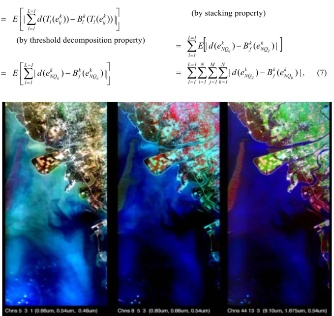
Fig. 12 MASTER images of different bands combination (left: RGB-bands 5-3-1, mid:RGB-bands8-5-3, right:

RGB-bands 44-13-3)

Figure 13. Classified map of the Au-Ku test site using GME/PBF-based multi-class classification method.

where a stack filter Sf (·), a threshold function T e (·) at level e, and a Boolean function B^kf(·) are used at each level. Furthermore, we can reformulate the CE value as the minimal sum over the 2ⁿ possible binary vectors of length n.

It will be a time-consuming procedure to find an optimal stack filter if n is a large number.

Referring to our previous work (Han, 1987), a graphic search-based algorithm further improves the searching process by utilizing the greedy and constraint satisfaction searching criteria. It guarantees that the output filter is a global optimal solution. Finally, a classification map, Ω, can be generated by this PBF-based multi-class classifier. The mechanism illustrated in Fig. 11 is an example of the use of the proposed PBF-based multi-class classifier to process a map classification. All PBF B^kf(·)of different classes at each level can simultaneously calculate the PBF binary outputs to classify a test sample.

The outputs of the stack filter, i.e. the summations of the PBF binary outputs at each level for each class ωk, are compared to each other and the one which has the smallest value is chosen as the final decision class for that test sample. This shows that our proposed PBF-based method can be used as a basis for a multi-class classifier.

3. EXPERIMENTAL RESULTS

The image data were obtained by the

MODIS/ASTER airborne simulator (MASTER) instrument, a hyperspectral sensor instrument, as part of the PacRim II project (Hook et al., 2001). The MASTER images of the test area with different band combination are displayed in Fig. 12. A plantation area in Au-Ku on the east coast of Taiwan shown in Fig. 13 was chosen for study. A ground survey was made of the selected six land cover types at the same time. The MASTER is most appropriate for this study because it is a well-calibrated instrument and it provides spectral data in the visible to shortwave infrared region of the electromagnetic spectrum.

The proposed PBF-based multi-class classification method was applied to 35 bands selected from the 50 contiguous bands of MASTER, excluding the low signal-to-noise ratio mid-infrared channels (Hook et al., 2001).

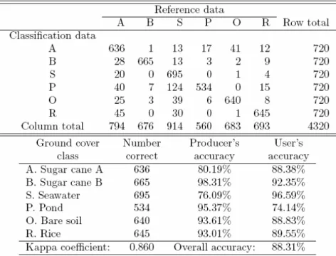
A, B, S, P, O and R stand for six ground cover classes, sugar cane A, sugar cane B, seawater, pond, bare soil and rice (N = 6). The criterion for calculating the classification accuracy of experiments was based on exhaustive test cases.

One hundred and fifty labeled samples were randomly collected from ground survey data sets by iterating every fifth sample interval for each class. Thirty labeled samples were chosen as training samples, while the rest were used as test samples, i.e. the samples were partitioned into 30 (20%) training and 120 (80%) test samples (M = 120) for each test case. Three correlation coefficient threshold values, tc =

0.75, 0.80 and 0.85, were selected to carry out GMET. Four different window lengths, n∈ {3,4,5,6}, were selected for each class. Based on PBF-based multi-class classification criteria, there were NM test samples (NM = 720) for each class. The cumulative percentages of eigenvalues were set as 90% to perform GME

projection and generate RRE vectors e^k. Finally, the accuracy was obtained by averaging all of the multiple combinations stated above. An example of an error matrix is given in Table 1 to illustrate the accuracy assessment of the PBF-based multi-class classification method.

Table 1. An example of an error matrix for clear boundary sampling. A summary of classification errors is appended below.

Two different traditional feature extraction techniques, minimum Euclidean distance (MED) and conventional PCA, were applied to the same PBF-based multi-class classifier for accuracy comparison. In Fig. 14, 5 GME specifies a window of fixed length five (n = 5) that was selected for each class. 5 EUB, 5 EAB and 5 ELB represent respectively the best five upper bound feature bands, the average five bands (between upper bound and lower bound) and the worst five lower bound

feature bands obtained by using the MED of the original data sets. 5 PCA stands for the first five principal components of PCA of the original data sets. As shown in Fig. 14, the accuracy rates are improved by enlarging the feature dimensions for GME and MED, but not those of PCA. It can be interpreted that the last few PCA components contain some global variances which can be treated as noise in MASTER data sets. Compared to MED and PCA, GME feature extraction is very suitable

for the PBF-based multi-class classifier in general.

There is a decline in accuracy rates for GME when six ground covers are selected.

This is caused by the fact that some classes of high-dimensional data sets have only a few effective modular eigenspaces Φ^kl inside their own GME set Φ^k. In Fig. 7, we can see that some ground cover classes, such as rice (R), have many ineffective modular eigenspaces Φ^k which have small numbers of feature bands ml in their GME set Φ^k. Note that we have previously sorted and reordered every Φ^kl in Φ^k according to their number of ml by descending order. If we choose a large window of length n, i.e. the top modular eigenspaces (Φ^k1,...Φ^kl,...Φ^nkk) of Φ^k, then some classes which have ineffective modular eigenspaces in n will be misclassified.

This is why the accuracy rates fall when the sixth ground cover class is included in Fig. 14.

It can be interpreted as a great benefit in that the GME provides a very useful pre-classification estimation measurement before we choose a proper window of length n for each training class as the parameters to build an efficient classifier.

Interestingly, we demonstrated a case in which there was a difference in classification accuracy between vague and clear boundary sampling. By vague boundary sampling we mean that some mixed pixels in the uncertain boundaries are chosen when we visually select labeled samples from the hyperspectral data sets. Conversely, clear boundary sampling

means that the chosen labeled samples are pure pixels without ambiguity. A vague version of a GME error matrix is shown in Table 2. It uses the same conditions as described above but applies to vague boundary sampling. Compared to Table 1, Table 2 has better classification accuracy. It proves that PBF-based multi-class classifiers do have more nonlinearly discrete capacity to increase class separability if vague boundary sampling is used to develop the classifiers.

The discrete and nonlinear properties of the proposed PBF-based multi-class classifier are considered to be advantages in classification. In Table 3, a summary evaluation of classification accuracies under different conditions illustrates the validity of these unique properties of proposed PBF-based multi-class classifiers.

The encouraging results have shown that an adequate classification rates, almost near 94%

average accuracy for the best case, are archived with only few training samples. Shown in Fig.

13 is an example of the classified map obtained by applying GME/PBF-based multi-class classification schemes to the MASTER high-dimensional data sets.

4. CONCLUSIONS

In this paper, a sophisticated GME/PBF-based multi-class classifier is proposed for hyperspectral supervised classification. We first introduce the GME which can be obtained

by a quick greedy band reordering algorithm. It is efficient with little computational complexity. The GME is built by grouping highly correlated bands into a small set of bands. The GME can be treated as not only a preprocess of the filter-based classifier but also a unique spectral-based feature set that explores correlation among bands for high-dimensional data. It makes use of the potential separability of different classes to overcome the drawback of the common covariance bias problems encountered in conventional PCA. The characteristic of GME is suitable for multi-class classifier. The proposed GME/PBF-based multi-class classifier enhances the separable features of different classes to improve the classification accuracy significantly. The conducted experiments demonstrated the validity of our proposed GME/PBF-based multi-class classification scheme.

The proposed PBF-based multi-class classifier is developed to effectively find nonlinear boundaries of pattern classes in hyperspectral data. Combining the GMET algorithm with the PBF-based multi-class classifier provides unique advantages for hyperspectral image classification. It possesses well-known threshold decomposition and stacking properties. The advantages of a PBF-based multi-class classifier are its discrete and nonlinear binary properties.

It utilizes the MCE learning ability to improve the classification accuracy particularly in

dealing with hyperspectral data sets in which training data are always inadequate and knowledge of the data distribution is usually incomplete. This MCE characteristic can best harmonize the PBF-based multi-class classifiers with the features extracted from GME. It improves classification accuracy significantly and fully promotes multi-class classifiers instead of pairwise classifiers.

The experiments validate the utility of the GME/PBF-based multi-class classifier. The highly correlated property of the GME can help us develop a suitable preprocessing algorithm for hyperspectral data compression.

Furthermore, we can take the benefits of the parallel property in GME to increase computation speed and achieve real time computation. These valuable advantages for practical implementation will be included in our future study.

ACKNOWLEDGMENTS

The authors would like to thank the Center for Space and Remote Sensing Research of National Central University for providing MASTER datasets used for experiments in this paper.

Figure 14. Classification accuracy comparison of three feature extraction techniques, GME, MED and PCA, using the same PBF-based multi-class classifier.

Table 2. Classification error matrix for vague boundary sampling. A summary of classification errors is appended below.

Table 3. Summary evaluation of classification accuracy for different boundary sampling types and number of modular eigenspaces.

REFERENCES

Dougherty, E.R., 1992, ”Optimal Mean-Square N-Observation Digital Morphological Filters. II. Optimal Gray-Scale Filters,”

CVGIP: Image Understanding, 55(1), pp.

55–72.

Duda, R.O. and Hart, P.E., 1973, ”Nonparametric Techniques,”

Pattern Classification and Scene Analysis, John Wiley & Sons, New York.

Han, C. C., Fan, K. C. and Chen, Z. M., 1997, ”Finding of optimal stack filter by graphic searching methods,” IEEE Trans.

Signal Processing, 45(7), pp. 1857–1862.

Han, C. C. and Tsai, C. L., 2001, ”A multi-resolutional face verification system via filter-based integration,”

IEEE Int. Carnahan Conf. Security Technology, pp. 278–281.

Han, C. C., 2002, ”A supervised classification scheme using positive boolean function,”

accepted for publication in International Conference on Pattern Recognition, IEEE, Quebec, Canada, pp. 100–103.

Harsanyi, J. and Chang, C.-I, 1994, ”Hyperspectral image classification and dimensionality reduction: an orthogonal subspace projection approach,” IEEE Trans.

Geosci. Remote Sens., 32(4), pp. 779–

785.

Hook, S. J., Myers, J. J., Thome, K. J., Fitzgerald M. and Kahle, A. B.,

2001, ”The MODIS/ASTER airborne simulator (MASTER) -a new instrument for earth science studies,” Remote Sensing of Environment. 76(1), pp.

93–102.

Jia, X. and Richards, J. A., 1999, ”Segmented principal components transformation for efficient hyperspectral remote-sensing image display and classification,” IEEE Trans. Geosci. Remote Sens., 37(1), pp.

538–542.

Jimenez, L. O. and Landgrebe,D.

A.,1999, ”Hyperspectral data analysis and supervised feature reduction via projection pursuit,” IEEE Trans. Geosci.

Remote Sens., 37(6), pp. 2653–2667.

Juang, B. H., Chou, W. and Lee, C. H., 1997, ”Minimum classification error rate methods for speech recognition,” IEEE Trans. Speech and Audio Processing, 5(3), pp. 257–265.

Kumar, S., Ghosh, J. and Crawford,M. M., 2001, ”Best-bases feature extraction algorithms for classification of hyperspectral data,” IEEE Trans. Geosci.

Remote Sens, 39(7), pp. 1368–1379.

Lee, C. and Landgrebe, D. A., 1993, ”Analyzing high-dimensional multispectral data,” IEEE Trans. Geosci.

Remote Sens., 31(4), pp. 792–800.

Lin, J. H. and Coyle, E. J., 1990, ”Minimum mean absolute error estimation over the class of generalized stack filters,” IEEE Trans. Acoust., Speech, Signal

Processing, 38, pp. 663–678.

Maragos, P. and Schafer, R. S., 1987, ”Morphological filters. Part II:

Their relations to median, order-statistic, and stack filters,” IEEE Trans. Acoustics, Speech, and Signal Processing, 35, pp.

1170–1184.

Moghaddam, B. and Pentland, A., 1995, ”Probabilistic visual learning for object detection,” in Proc. 5th International Conference on Computer Vision, Boston, MA., pp. 786–793.

Pentland, A. and Moghaddam, B., 1994, ”View-based and modular eigenspaces for face recognition,” IEEE Computer Society Conference on Computer Vision and Pattern Recognition, pp. 84–91.

Postaire, J.G., Zhang R.D. and Lecocq-Botte, C., 1993, ”Cluster analysis by binary morphology,” IEEE Trans. Pattern Analysis and Machine Intelligence, 15, pp. 170–180.

Richards, J. A. and Jia, X., 1999, ”Interpretation of Hyperspectral Image Data,” Remote Sensing Digital Image Analysis, An Introduction, 3rd ed., Springer-Verlag, New York.

Wendt, P. D., Coyle, E. J. and Gallagher, N. C., 1986, ”Stack filter,” IEEE Trans.

Acoustics, Speech, and Signal Processing, 34(4), pp. 898–911.

一個新穎的方法實現高光譜監督式遙測影像分類

張陽郎

¹

韓欽銓

²

范國清

³

陳錕山

⁴

摘要

「高光譜」遙測影像 (Hyperspectral Imagery) 為遙測影像之先進技術，遙測影像頻譜解析度由原數 個頻譜解析度的一般感測器、至數十個頻譜解析度之「多頻譜感測器」(Multispectral)、到數百個頻譜解 析度的「高光譜感測器」(Hyperspectral)、乃至於數千個頻譜解析度之「超高光譜感測器」(Ultraspectral)，

持續地進步演進著。「高光譜」解析度感測器已廣泛應用於衛星遙測影像之識別、醫學影像的診斷、工

業產品之檢驗、飛機及其他精密機器設備之非破害性檢查等應用上，「高光譜」遙測影像技術業已成為

遙測影像中一個新興且重要的研究領域。本文提出一個適用於「高光譜」遙測影像分類的新演算法，

主要有兩個實現步驟，第一個步驟為「貪婪模組特徵空間」(Greedy Modular Eigenspaces)，第二為「布 林濾波器」(Positive Boolean Function)。藉由校正過後的完整台灣『高光譜』遙測影像資料，以及實地 測量的地表真實資料，來實際證明「貪婪模組特徵空間」的方法提供了一個絕佳的特徵抽取方式，並 為一個最適合「布林濾波器」分類方法的前處理器。本文詳細討論「貪婪模組特徵空間」演算法之推 導、完整描述「布林濾波器」的基礎理論，以及詳細分析他們之間的關係，並針對二者的特性加以推 演，提出適用於一般「高維資料」(High-Dimensional Data)資料分類的解決方法。最後經由實驗驗證並與 其他傳統「多頻譜感測器」遙測影像資料分類方法作一比較，印證了本方法非常適用於「高維資料」

分類的特性。

關鍵字: 主軸分析、高光譜監督式分類、貪婪模組特徵空間、布林函數、堆疊濾波器

1.國立臺北商業技術學院資訊管理系副教授

2.國立聯合大學資訊工程學系副教授

3.國立中央大學資訊工程學系暨研究所教授

4.國立中央大學太空及遙測研究中心暨太空科學研究所教授

收到日期:民國 92 年 11 月 11 日 修改日期:民國 93 年 07 月 25 日 接受日期:民國 93 年 07 月 27 日