在8 TeV質心能量的質子對撞實驗中尋找頂夸克透過Z玻色子及魅夸克（或上夸克）衰變的事件

(1)

國立臺灣大學理學院物理學系碩士論文

Department of Physics College of Science

National Taiwan University Master Thesis

在 8 TeV 質心能量的質子對撞實驗中尋找頂夸克透過 Z 玻色子及魅夸克（或上夸克）衰變的事件

Search for top decays through flavor changing neutral current process, , in pp collisions at √

李昀翰 Yun-Han Lee

指導教授：張寶棣教授 Advisor: Pao-Ti Chang, Prof.

中華民國 102 年 6 月 June, 2013

(2)

19

(3)

摘要

在標準模型中，按照 GIM 機制的預測，以 Z 玻色子為媒介之跨世代衰變反應是被抑止的，在頂夸克的例子中，其反應率遠低於目前之測量範圍，但在其它模型中，該反應率可以目前之測量範圍。

我們使用了緊湊渺子線圈在2012 年紀錄的質心能量為 8 TeV 之質子對撞數據，

總通量約為19.5 fb^-1，以尋找頂夸克衰變至Z 玻色子與魅夸克(或上夸克)的事件。

在大強子對撞機實驗中，大多數頂夸克係成對產生，故我們以tt̅ → Wb + Zq之輕子性衰變為尋找標的，即W 玻色子衰變至電子或渺子及對應的微中子，Z 玻色子衰變為電子或渺子對。我們使用了b 簇射(jet)標記，以配對衰變至 Wb 的頂夸克，以反b 簇射標記配對衰變至 Zq 的頂夸克。在此選擇條件下，背景之主要組成為Ztt̅以及 WZ 反應。

我們以b 簇射標記法進行數據導向之背景分析，預測將觀測 3.08±0.85±0.76 個背景事件，與蒙地卡羅法之預測一致。

在數據中僅觀察到一個滿足選擇條件的事件，符合標準模型之預測；我們計算出t → Zq之衰變佔頂夸克衰變的百分率在 95%之信心水準下不超過 0.06%。

關鍵詞：GIM 機制、大強子對撞機、緊湊渺子線圈、味變中性流、頂夸克

(4)

Abstract

In the standard model, cross-generation interactions mediated by Z bosons, known as the flavor-changing neutral current (FCNC), are highly suppressed. For top quark FCNC decay, the cross-section is far below the experimental limit. However, other models predict much higher cross- sections, and some of them are even within reach. Therefore, using the data sample corresponding to an integrated luminosity of 19.5 f b⁻¹ proton-proton collisions at a center-of-mass energy √

s = 8T eV , col-

lected with the CMS detector at the LHC, we performed the search with the decay chain t¯t to Wb+Zq, where W decays to a charged lepton and a neutrino and Z decays to two charged leptons. The data-driven analysis using b-tagging method is performed with the estimated background be- ing 3.08 ± 0.85±, which is consistent with the estimation of Monte-Carlo method. One event is observed in the data which is consistent with the expected background, and the upper limit of the branching fraction for t → Z+q is calculated as 0.06% at the 95% confidence level.

Key words: GIM mechanism, LHC, CMS, FCNC, top

(5)

List of Figures

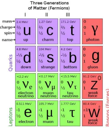
1.1 A summary table of currently known elementary particles. The mass

is labeled in natural unit. . . 15

1.2 The tree diagram (left) is suppressed in SM, while the loop diagram (right) is of very small cross section. . . 16

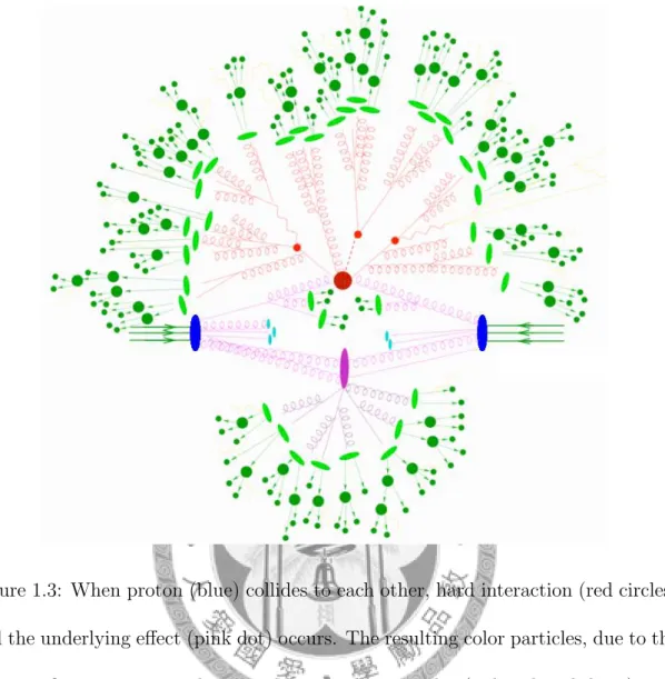
1.3 When proton (blue) collides to each other, hard interaction (red circles) and the underlying effect (pink dot) occurs. The resulting color particles, due to the color confinement, copiously creates more color particles (red and pink lines), and finally, all color particles binds together to form hadrons (green). . . 19

1.4 The gluon fusion is the main mechanism of top production in LHC experiment. . . 19

2.1 A plot showing the process of acceleration of protons. Four interaction points symboling different detectors are also shown in the plot, and the top one is the CMS detector. . . 21

2.2 The CMS detector. . . 22

2.3 The quarter view of the inner tracking system. . . 24

2.4 The quarter view of the muon chamber. . . 25

2.5 The quarter view of the ECAL crystals. . . 26

(9)

2.6 The quarter view of the ECAL, HCAL and the muon chamber. . . 27 2.7 The transverse view of CMS detector which summarize the methods

for identifying different particles. . . 28

3.1 The resolution of pt and impact parameter of tracks. . . 30 3.2 The material budgets leads to energy loss of electrons. . . 31 3.3 Combining the ECAL and tracking information, a good resolution

can be obtained in different pt region. . . 32 3.4 The standalone (left) muon and global (right) muon reconstruction

efficiency. . . 33 3.5 The standalone (left) muon and global (right) muon reconstruction

resolution. . . 34 3.6 The resolution of MET. . . 35 3.7 The resolution of jets in different region. . . 37 3.8 The discriminating variable of CSV for different types of jet. The

solid, dotted, and dashed lines are the b, c and light quarks respectively. 38

4.1 An event after reconstruction. The green lines are the tracks of charged particles and the yellow dots are the vertices. . . 42 4.2 The pile-up distribution of the Run2012A data and the distribution

assigned for MC production in 2012 summer. The division of these two gives the proper weights for different number of interaction. . . . 42

5.1 The vertex DoF (left) and the number of vertex (right). . . 46 5.2 After Z selection, the pt (left) and eta (right) distributions of electrons. 47 5.3 After Z selection, the pt (left) and eta (right) distributions of muons. 48

(10)

5.4 After Z selection, the pt (left) and eta (right) distributions of jets. . . 48 5.5 After Z selection, the pt (left) and mass (right) distributions of Z

candidates in electron channel. . . 49 5.6 After Z selection, the pt (left) and mass (right) distributions of Z

candidates in muon channel. . . 49 5.7 After Z and W selection, the W transverse mass (left) and the MET

(right) distributions. . . 50 5.8 Before the mass window selection, the top Wb (left) and Zj (right)

mass distributions. . . 51 5.9 The ∆φ distribution of top pair. . . 52 5.10 The mass correlation distribution in data with the red dotted box

labels the mass window. One sees that after applied all the selection, one event falls in the desired mass window. . . 52

6.1 The tree diagram showing the weight of each combination for a ttZ event. The acceptance is evaluated as 74% using ttbar MC sample. . 56 6.2 The toy study shows the sigma of NBKG is 0.85. . . 59

7.1 The U_n to Z’s pt (left) and U_p to Z’s pt (right) distributions. . . 63

(11)

List of Tables

4.1 The data used in this analysis and the corresponding integrated luminosity. . . 41 4.2 The MC sample used in this analysis . . . 43

5.1 Summary of data yields after each cuts applied in sequential. . . 53

6.1 The combination considered for each process. Where l can be u, d, s quarks or gluon. Since four quarks are expected in ttZ, further investigation considering jet acceptance is performed. . . 55 6.2 The probability for each combination to have exactly one b-tagged. . 57 6.3 The probability for each combination to have exactly zero b-tagged. . 58 6.4 The expected SM background contributions with 19.5 f b⁻¹ data. . . . 60

7.1 Summary of uncertainties from MadGraph parameters. . . 65 7.2 The uncertainty of different sources for signal efficiency estimation. . 67

(12)

7.3 The uncertainty of different sources for background estimation using data-driven method. The most significant source is b-tagging efficiency, which is estimated by varying the b-tagging efficiency by one sigma and re-construct the data-driven matrix. The second one is that from JES, JER and Pile-Up, which affect the top mass selection efficiency. . . 68 7.4 The uncertainty of different sources for background estimation using

MC method. . . 69

8.1 Background composition, observed and expected yields, and limits at the 95% CL for all three-lepton channels combined tag selections for an integrated luminosity of 19.5 f b⁻¹. The uncertainties in the background estimation include the statistical and systematic components separately (in that order). . . 71

(13)

Chapter 1 Introduction

1.1 The Standard Model

The Standard Model is a model developed to describe all known interactions between elementary particles: quarks, leptons and gauge bosons.

1.1.1 Quarks

There are six quarks labeled by different flavors. They are categorized in three generations. The lightest quarks, up quark and down quark, forms the everyday particles like neutrons and protons. They form the first generation. In the end of 1947, the discovery of kaon leads to the idea of strange quark. As the energy scale grows in experiments, more heavy particles were found. The heaviest quark, which is the top quark found two decades ago, is almost 175 times the proton mass.

Strange and charm quarks form the second generation; top and bottom quarks form the third generation. Quarks are fermions with spin ¹₂. The up, charm and top quarks carry charge +²₃; the down, strange, and bottom quarks carry charge -¹₃.

(14)

Each quark and gluon carry certain color, it can be blue, red or green (virtually).

They obey the rule of color confinement, which states that the color particle cannot exist alone in the nature. Therefore, to form a colorless particle, it must be either formed by three quarks or a quark plus an anti-quark. The former is called a baryon and the later is called a meson. The collection of these two are called hadrons.

The nature adapts the rule of baryon number conservation, which states that in a process, the number of baryon cannot change.

1.1.2 Leptons

There are six leptons labeled by their flavors. They can be separated by two cat- egories: charged leptons, which are the electron, muon and tauon, carrying charge -1, and the neutrinos, which are the electron neutrino, muon neutrino and the tauon neutrino, being charge neutral. With their name they also form three generations.

Different from quarks, leptons are colorless, so they are not involved in the strong interaction. Neutrinos are chargeless, so the only interaction for them is the weak interaction, which makes them hard to detect. Leptons obey the rule of lepton number conservation, which states that in any processes, the lepton number cannot change.

The lepton number is defined as the number of leptons in certain generation; e.g., the electron and electron neutrino are of lepton number 1, and their anti-particles are of -1.

1.1.3 Gauge Bosons

The four gauge bosons are photon, gluon, Z and W. The former two are massless.

The mass of Z boson is 91.2 GeV while the mass of W boson is 80.4 GeV. Only

(15)

gluon carries color, and only W carries charge, which can be +1 or -1.

Photon is the mediator of electromagnetic interaction; particles of charge like quarks and charged leptons participate in this interaction. Gluon is the mediator of strong interaction, all quarks are involved in this interaction since all of them carry colors. The W and Z bosons are the mediators of weak interaction, which effect all particles. Since neutrinos carry neither color nor charge, they only participate in the weak interaction, thus making them hard to be detected.

Figure 1.1: A summary table of currently known elementary particles. The mass is labeled in natural unit.

(16)

1.2 The Flavor-Changing Neutral Current of top decay

The interaction mediated by a Z boson (or Higgs boson) is called the neutral current.

In the Standard Model, if the quarks or leptons involved in the neutral current is of different flavor, the process will be suppressed. Such processes are called the flavor-changing neutral current.

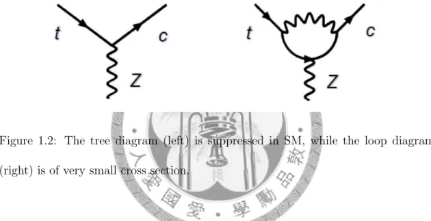
Figure 1.2: The tree diagram (left) is suppressed in SM, while the loop diagram (right) is of very small cross section.

In this analysis, we aim to search signal of the top quark decaying to Z and another light quark (charm or up). The tree level diagram is suppressed according to the GIM mechanism[1], and the loop diagram is of extremely small cross section.

The branching ratio of this process is of the order of magnitude of 10⁻¹⁴as predicted by the Standard Model, which means the detection of this process can be a hint of new physics. Other models (referred to as extended or beyond SM, ESM or BSM) predict a higher branching ratio and some are possible to detect in LHC experiment.

These models include the quark-singlet models[2], two-Higgs doublet models[3], R- violating Supersymmetry model, Technicolour model[4] and so on.

(17)

1.2.1 The two-Higgs doublet models

The two-Higgs doublet models predicts more than one Higgs boson and two of them are oppositly charged. These two oppositely charged Higgs boson provides a possible loop for the t → Z + q process, and may have a branching ratio of the order of magnitude of 10⁻⁶.

1.2.2 Supersymmetry models

The supersymmetry models predicts a new symmetry in which every known fermion and boson is of a ‘super partner’ of different spin; i.e., for fermions, their partners are bosons, and for bosons, their partners are fermions. There are many different types of supersymmetry models, and the simplist one is called the minimal supersymmetric standard model. In this model, the R-parity is introduced. In the model which R- parity is violated, the t → Z + q branching ratio can be as large as 10⁻⁴.

1.2.3 Technicolour model

In this model, a different particle (mechanism) is introduced in replace of the Higgs boson for the electroweak symmetry breaking issue. This model also provides ex- planation of the large top quark mass. The t → Z + q branching ratio can be as large as 10⁻⁵.

1.3 Proton-Proton Collisions

It is said that the proton-proton collisions are like throwing trash cans together. It is because the protons are not elementary particles, it is composed of valence quarks,

(18)

two up and one down quarks, and of many gluons and sea quarks. When two proton collides with very high momentum transfer, often, we would expect a parton from one proton and another parton from the other proton interacts, which we call it hard interaction. The hard interaction may creates quarks, leptons, or gauge bosons;

some are of color, and some are colorless. The rest part of the protons that did not participate the hard interaction sure are of color. With color confinement, these color particles quickly create many more color particles until they reach colorless state, this is what we refer to as ‘fragmentation.’ After the massive emergence of these color particles, they binds together and form a great amount of hadrons, which is called the ‘hadronization.’ Among the messy particles, the interesting one that most of the analysists focus on is the hard interaction, and those other interactions are referred to as the underlying events which are generally regarded as the noise contributor.

1.4 Strategy

The Large Hadron Collider provides events with the high energy collisions of protons, and therefore most of the top quarks are pair-produced through the gluon fusion.

More than 99% of the top quark decays to b quark and W boson, so in our analysis, we search for one decaying to W+b and the other to Z+q in the full leptonic decay channels, where Z then decays to two electrons or muons and W decays to electron or muon with the corresponding neutrino. This channel is relatively clean since it consists of three leptons in the final state. However, the cleanness also makes the rare processes like ttZ, tbZ non-negligible. The analysis steps will be provided in chapter five with more details.

(19)

Figure 1.3: When proton (blue) collides to each other, hard interaction (red circles) and the underlying effect (pink dot) occurs. The resulting color particles, due to the color confinement, copiously creates more color particles (red and pink lines), and finally, all color particles binds together to form hadrons (green).

Figure 1.4: The gluon fusion is the main mechanism of top production in LHC experiment.

(20)

Chapter 2 Experimental Apparatus

This chapter provides the description for the apparatus, which includes the collider and the detector.[5]

2.1 The Large Hadron Collider

The Large Hadron Collider, short as LHC, is a proton-proton collider with designed

√s = 14 TeV. The acceleration is achieved in several steps: the proton bunches are

first sent to the Linear accelerator to reach 50 MeV, followed by the Proton Syn- chrotron which raises the energy to 26 GeV. The beam is subsequently accelerated to 450 GeV in the Super Proton Synchrotron (SPS) and finally transferred to the LHC to reach the desired energy 7 TeV. On average, each bunch contains roughly 10¹¹ protons with bunch lenth being 7.55 cm and radius 16.6 µm. To control the beam, superconducting magnets are exploited with a temperature of 1.9 K. The Radio-Frequency system works to accelerates the particles and compensates energy loss due to synchrotron radiation. In such a high energy proton-proton collision, the QCD processes give enormous background to the experiment. In addition, the

(21)

high luminosity makes the radiation damage become an important issue in detector development.

Figure 2.1: A plot showing the process of acceleration of protons. Four interaction points symboling different detectors are also shown in the plot, and the top one is the CMS detector.

2.2 The Compact Muon Solenoid

There are six experiments operating at the LHC. Two of them, which are the CMS, short for the Compact Muon Solenoid and ATLAS, short for A Toroidal LHC Appa-

(22)

ratuS, are aimed for the high pt physics. They search for the physics of and beyond the Standard Model. One of the major goal is to search for the long-predicted Standard Model Higgs, which, in July 2012, had already gave the world impressive results. The CMS detector is featured by its muon system as well as the inner tracking system, together they make CMS capable for fine measurements of the charged particles. Other main components are the electromagnetic calorimeter (ECAL), the hadronic calorimeter (HCAL), and the solenoid which provides 3.8 T magnetic field, through which the measurement of the momentum of charged particles can be made.

Figure 2.2: The CMS detector.

2.2.1 Coordinate Conventions

By convention, the nominal collision point is taken as the origin, with the y-axis pointing vertically upward, the x-axis pointing radially inward toward the center of the LHC and the z-axis pointing along the beam direction. The azimuthal angle is defined as the angle between the projection (on x-y plane) of the vector and the

(23)

x-axis. The polar angle is defined as the angle between the vector and the z-axis.

The pseudo-rapidity is defined using the polar angle by η = −lntan(θ/2). The cylindrical part of the detector is also referred to as the barrel, while the plates at the two ends are known as the endcaps.

2.2.2 Magnet

In the CMS detector, the magnetic field of 3.8 T is provided for the measurement of the momentum of charged particles. The high-purity aluminium-stabilised conductor and indirect cooling (by thermosyphon), together with full epoxy impregnation are used.

The overall conductor cross section is 64 × 22 mm². The conductor was manu- factured in twenty continuous lengths, each with a length of 2.65 km. Four lengths were wound to make each of the 5 coil modules.

2.2.3 Inner Tracking System

The tracking system using silicon sensors provides the measurements of the track and thus the momentum of charged particles. It consists mainly three regions. The detectors in the innermost region locates roughly 10 cm from the center cylindrically, the detectors here are also known as the pixel tracker due to their fine resolution.

In the intermediate region where 20 < r < 55 cm, are another set of the detectors with less resolution. In the outermost region where r > 55 cm lays the larger-pitch detectors. The later two are known as the strip tracker, and are called TIB (Tracker Inner Barrel) and TOB (Tracker Outer Barrel), respectively. The pixel detector consists of 3 barrel layers with 2 endcap disks on each side on them. The 3 barrel

(24)

Figure 2.3: The quarter view of the inner tracking system.

layers are located at mean radii of 4.4 cm, 7.3 cm and 10.2 cm, and have a length of 53 cm. The second disks, extending from 6 to 15 cm in radius, are placed on each side at |z|= 34.5 cm and 46.5 cm. The spatial resolution of the pixel detector is about 10 µm for the r-φ measurement and about 20 µm for the z measurement.

The TIB is made of 4 layers and covers up to |z|< 65 cm while the TOD comprises 6 layers with a half-length of |z|< 110 cm. The TEC (Tracker End Cap) and TID (Tracker Inner Disks) locate at the endcaps. Each TEC comprises 9 disks that extend into the region 120 cm<|z|< 280 cm, and each TID comprises 3 small disks that fill the gap between the TIB and the TEC. Starting from inside, the resolution of these strip detectors vary from 23-52 µm for the r-φ measurement and 230-530 µm for the z measurement.

2.2.4 Muon System

For the low momentum muon, the inner tracking system can provide good measurement; while for the high momentum ones the uncertainty become large due to the curvature being small. On contrary, the muon chamber locates in the outer region

(25)

can measure high momentum muons to a good precision while the low momentum ones, being scattered by the materials, cannot be well measured. Therefore, with both tracking system and muon chamber (full system), the capability of muon measurement of CMS is excellent. In muon chamber, three types of detectors are used:

the drift tube, which covers the region | η |< 1.2, the cathode strip chambers, which covers the region | η |< 2.4, and the resistive plate chambers, which covers the region 0.8 <| η |< 2.4. These detectors are chosen depending on the environment of the magnetic field and the radiation of their location.

Figure 2.4: The quarter view of the muon chamber.

2.2.5 Electromagnetic Calorimeter

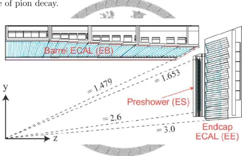
The electromagnetic calorimeter (ECAL) measures the energy of charged particles and photons. It is made of lead tungstate crystals with short radiation length (0.89 cm), fast response (80% of the light is emitted within 25 ns) as well as good radiation

(26)

resistance. The silicon avalanche photodiodes (APDs) and the vacuum phototriodes are used as photodetectors in the barrel and endcap region, respectively.

The ECAL in the barrel region, short as EB, covers the region of 0 <| η |< 1.479 with a total radiation length corresponding to 25.8 X0. The front face of the crystal in EB is about 22 × 22 mm². The ECAL in the endcap region, short as EE, covers the region of 1.479 <| η |< 3.0. They have a front face cross section of 28.6×28.6 mm² and a length of 220 mm (24.7 X0). Locating in front of EE, the preshower detector composed of silicon sensors aims to separate the photon of Higgs decay from those of pion decay.

Figure 2.5: The quarter view of the ECAL crystals.

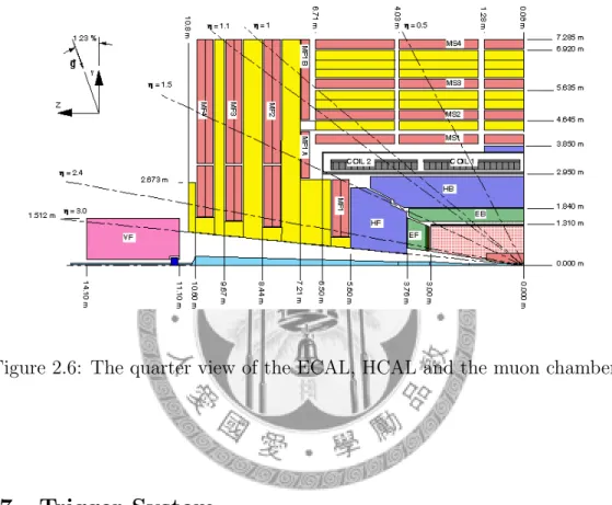
2.2.6 Hadron Calorimeter

The hadron calorimeter (HCAL) measures the energy of hadrons. It is made of brass which provides short interaction length and considerably small magnetic response.

The plastic scintillator tiles read out with embedded wavelength-shifting (WLS) fibres are exploited.

The HCAL is separated into several regions: the barrel region, called HB, cov-

(27)

ering the pseudo-rapidity region −1.4 < η < 1.4, with segmentation ∆η × ∆φ = 0.087 × 0.087, the outer region, called HO, covering the region −1.26 < η < 1.26, and the endcap region, called HE, which covers the region 1.3 <| η |< 3.0. As for 3.0 <| η |< 5.0, the stell/quartz fibre forward calorimeter (HF) is used, whose also provide the luminosity measurement.

Figure 2.6: The quarter view of the ECAL, HCAL and the muon chamber.

2.2.7 Trigger System

Due to the high luminosity in the LHC, it becomes very important to have a mature trigger system. There are four major components in the CMS trigger system: the detector electronics, the Level-1 trigger processors (calorimeter, muon, and global), the readout network, and an online event filter system (processor farm) that executes the software for the High-Level Triggers (HLT).

The Level-1 trigger makes calculations in less than 1 µs, while the time it takes for the transit is 3.2 µs. A large fraction of events are discarded, only 1 crossing in 1000 is kept. When the Level-1 functioning, the high-resolution data is held in

(28)

pipelined memories. Commodity computer processors make subsequent decisions using more detailed information from all of the detectors in more and more sophis- ticated algorithms that approach the quality of final reconstruction. The ideal rate of L1 is 100 kHz. Afterwards, the data will be sent to the DAQ system with each event roughly 1.5 MB contained in hundreds of buffers. Then the processor runs the high-level trigger which reduce the rate to 100 Hz and then sends them to storage system. The separation of the L1 and HLT allows more flexible update for the HLT.

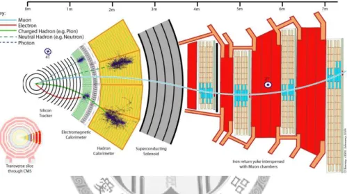
Figure 2.7: The transverse view of CMS detector which summarize the methods for identifying different particles.

(29)

Chapter 3 Physical Object Reconstruction

The physical objects used in this analysis include tracks, vertices, electrons, muons, the transverse missing energy and jets. The b-tagging algorithm is described as well.

3.1 Track Reconstruction

The connection of points of signals left on the tracking system gives tracks. The parameters of a track, which are the curvature, the impact parameter, the azimuthal angle, and the pseudo-rapidity, should be obtained in mainly three steps: seeding, building and fitting. The seed, which is the staring point, of track reconstruction, is the signal left on the pixel sensors. Due to the number of free parameters, at least two hits are required for deciding a track. Then, to build up the track, the outer layer is checked one by one to collect all the compatible hits and form track candidates. Finally, to avoid bias from the seeding constraints, an overall fitting is needed. The standard Kalman filter and smoother are used in this stage.

(30)

Figure 3.1: The resolution of pt and impact parameter of tracks.

3.2 Vertex Reconstruction

The information of track can be used to obtain the vertex information. Vertex consists of the following free parameters: position, covariance matrix, and track parameters constrained by the vertex position and their covariances. The reconstruction of vertex is done through two steps: finding and fitting.

In the finding step, four sub-steps are involved: preselection, formation, fit, exclusion. First, the tracks with small impact parameter and pt > 1.5 GeV are chosen; then, clusters of tracks are formed according to their impact parameter along z-axis. Using these clusters, a fit is made to determine the vertex. What followed is the exclusion step where the bad fits are dropped. During the compatibility calculation, the Gaussian resolutions are assumed.

In the fitting step, the most often used algorithm is the Kalman filter (KVF).

Mathematically, it is equivalent to a global least-squares minimization. This filter can also be used to improve estimation of the track momenta with constrains.

(31)

3.3 Electron Reconstruction

To reconstruct electrons, whose four-momentum should be decided, the information of tracking system and electromagnetic calorimeter (ECAL) is needed. The issue of energy loss is considered because of the materials in the tracking system. About 50%

of the cases the electrons will radiate more than 50% of its energy before reaching ECAL. Another issue is that the electrons may come from the conversion of photons, which leads to the showering patterns.

Figure 3.2: The material budgets leads to energy loss of electrons.

The steps can be separated to two parts: seeding and fitting. The seeding uses the information in the ECAL. ‘Hybrid’ and ‘island’ superclustering algorithms are use in determining the ECAL information in barrel and endcaps respectively. With low threshold of the energy of supercluster, the efficiency of seeding can be as high as 99% for electrons with pt higher than 7 GeV/c. The supercluster information will then be combined with the pixel detector to decide the two pixel hits needed for track finding.

(32)

The benefit of combining the information of ECAL and tracking system is based on the fact that the energy weighted average impact point of the electron and associ- ated bremsstrahlung photons, as calculated using information from the supercluster in the ECAL, coincides (assuming a successful collection of photons) with the impact point that would have been measured for a non-radiating electron of the same initial momentum.

In the fitting stage, the problem of radiation energy loss made it important to have an improved tracking algorithm especially for those low pt electrons. The nonlinear Gaussian Sum Filter is thus introduced to make up the short coming of the Kalman filter. The average efficiency of the electron reconstruction is above 90%.

Figure 3.3: Combining the ECAL and tracking information, a good resolution can be obtained in different pt region.

(33)

3.4 Muon Reconstruction

The reconstruction of muon uses the information of muon system and the inner tracking system, and the step can be divided into local reconstruction, standalone reconstruction and global reconstruction.

The local reconstruction is done using the information of the CSC and DT detectors which decide the track segment for further reconstruction.

The standalone reconstruction uses only the information in the muon system.

The track segment obtained in previous step will be combined with outer layer information using the Kalman-filter. Then a backward fit is performed to decide the vertex from which the muon comes.

In the final step, which is the global reconstruction, the inner tracking system information is exploited together with what was obtained in the standalone step. In this step, the muon track will be extrapolated to the tracking system and then the corresponding hits will be used to optimize the momentum measurement.

Figure 3.4: The standalone (left) muon and global (right) muon reconstruction efficiency.

(34)

Figure 3.5: The standalone (left) muon and global (right) muon reconstruction resolution.

3.5 Particle Flow and Transverse Missing Energy

The particle flow is used during the reconstruction. It is based on the idea that one should include all detectors when doing the reconstruction of stable particles like electrons, muons, photons, hadrons (mainly pions and kaons). The list of particles will then be used to reconstruct jets as well as the transverse missing energy (short as MET).

The basic treatment is to use the tracks of charged particles and the clusters which is the energy left in the calorimeter as building blocks and reconstruct the particles as a whole.

Due to the well-functioning of the muon system, muons are first reconstructed and the corresponding blocks are removed from the list. What follows is the electron since it has little to do with the jet and MET reconstruction. Then the clusters and tracks related to the electrons are removed including those coming from the electron bremsstrahlung. The remaining tracks will be used to form charged hadrons candidates. What are left are the neutral particles with clusters energy deposit not

(35)

being able to match the track information. These are used to reconstruct the photon and the neutral hadrons. After all these one has filled a list of particles that may be used for the reconstruction of jets.

The MET the unbalanced energy on the transverse plane that coming from the neutrino or other weakly interacting particles created in the collision that cannot be detected. With the particle flow procedure, it is then straightforward to determine the MET: vector sum over all reconstructed particles in the event and then taking the opposite of this azimuthal, momentum two-vector.

Figure 3.6: The resolution of MET.

3.6 Jet Reconstruction

In this analysis jets are referring to the product of the hadronization of the color particles; due to the color confinement, when a particle with color is created, it will

(36)

massively produce pairs of color particles until the color is balanced. These color particles will then form many hadrons and result in a jet signature. It is through clustering these hadronized particles that a jet is reconstructed.

There are many ways to do the clustering, and the algorithms frequently used are the k_T, Cambridge/Aachen and the anti-k_T methods. The one used in this study is called anti-k_t algorithm.

First, the distance variables are defined as:

dij = min(k_{T i}^2p, k^2p_{T j})∆²_ij R²,

d_iB = k_{T i}^2p,

where R is a parameter often set as 0.5. k_T is the transverse momentum, and the B indicates the beam. p is another parameter to be considered.

We collect all the possible candidates, either hadrons or the signal left in the calorimeter. Then this formula is applied to calculate the distance between two candidate i and j. If d_ij is larger than d_iB, then the two candidates are merged.

Else, the candidate is preserved for other clustering.

The parameter p in the formula categorizes the methods. The p = 1 case is the k_T method, the p = 0 case is the Cambridge/Aachen method, and the p = −1 is the anti-k_T method.

The energy measured should be further corrected in the sense that there should be non-negligible loss of energy. The energy correction is done by several steps.

The first step, called the Level 1 correction, is applied for the noise and pile-up suppression, and followed by the level two correction, which corrects the energy shift due to different η direction. And finally the level three correction corrects the pt to the ideal value when it is created[11].

(37)

Figure 3.7: The resolution of jets in different region.

3.7 b tagging

In order to search the FCNC signal which contains one b quark in the pattern, the b-tagging technique is used for identifying if the jet is originated from a b quark (short as b jet).

This identification exploited the relatively long life time of b quark, which makes the vertex of a b jet shift from the primary vertex. Therefore, high spatial resolution track is of great importance.

In this analysis, the Combined Secondary Vertex method is used for b jet identification. First, the charged tracks in a jet are collected, and then the Trimmed Kalman Vertex Finder is exploited which selects the outliers of the tracks that can be used for secondary vertices reconstruction. Then the reconstructed secondary vertices’ parameters and the tracks’ parameters will be combined as a discriminating variable.

(38)

Figure 3.8: The discriminating variable of CSV for different types of jet. The solid, dotted, and dashed lines are the b, c and light quarks respectively.

(39)

Chapter 4 Data and Monte Carlo Samples

The data used in this analysis is collected with CMS detector from the LHC de- livered 2012 8 TeV proton-proton collision. The double electron and double muon triggered data are used with corresponding integrated luminosity of 19.5 f b⁻¹. With the help of computing elements, it is also possible to generate the events which sim- ulate the proton collisions and the detector response. In event generation, the first step is the parton level generation carried out by MadGraph 5[6] event generator, which performs the tree level calculation of a physical process using the helicity method[7]. Besides the process in standard model, MadGraph is also capable of doing calculation through a user-defined model. Then the output will be sent to PYTHIA 6[8] generator for the fragmentation and hadronization. TAUOLA[9] is also used for the emulation of tauon decay. The generated event will be sent to the GEANT 4 detector simulator which simulates the detector response. The first step is called generation, and the second step is called simulation. We refer to this sample as MC sample.

The MC sample is generated separately of different processes, while in data all

(40)

kinds of processes are mixed. Therefore, if we combine all the MC sample, it is possible that it can represent the result in data, and we can further estimate the fractions and distributions of different processes with different physical variables.

Also, with MC sample we can determine the proper way to separate the signal process from the background and can have much higher statistics, for the event number in data is limited by the apparatus.

The FCNC MC signal MC sample contains the ttbar process where one of them decays to q (which may be c, cbar, u and ubar) and Z, while the other decays to b (or bbar) and W. Then the Z and W bosons decay to leptonic final states. Setting the branching ratio of this process to be 0.1%, we can then calculate the cross-section of this sample to be 0.047 pb. The sample contains equal amount of t to Zc and t to Zu events.

The other standard model background included in the study are the W, Z, WW, WZ, ZZ, ttbar, ttbarZ, ttbarW, and single top. Among them, the major contribution comes from WZ and ttbarZ events which have very similar pattern comparing to FCNC in the desired final states. The table below summarize the sample used in this analysis.

4.1 Pile-Up Treatment

The LHC collisions are of extremely high luminosity. In 2012, there are often more than 20 interactions per event; although these events are of relatively small momentum transfer, the resulting energy deposit will be non-negligible. Therefore, on one hand, it is of great importance to model the pile-up effect in the MC simulation, while on the other hand, it is very crucial to reduce noise from pile-up effect.

(41)

Data Int. Lumi. (pb⁻¹) DoubleElectron(Muon) Run2012A-13Jul2012-v1 808.47 DoubleElectron(Muon) Run2012A-recover-06Aug2012-v1 82.14 DoubleElectron(Muon) Run2012B-13Jul2012-v1 4428.67 DoubleElectron(Muon) Run2012C-24Aug2012-v1 495.00 DoubleElectron(Muon) Run2012C-PromptReco-v2 6401.67 DoubleElectron(Muon) Run2012D-PromptReco-v1 7273.70

Total 19489.65

Table 4.1: The data used in this analysis and the corresponding integrated luminosity.

We use the number of interaction to describe the pile-up effect. For an event with high number of interaction, the pile-up is severe, while for an event with low number of interaction, the pile-up is not significant. The number of interaction is a probability function and in the 2012 Run period A, the most probable value is around 15. To model the pile up effect in the MC sample, the general approach is overlapping the low energy interactions several times with some shifts on the hard process. The probability function of the number of interaction varies with the luminosity; therefore, one first assign a probability function similiar to but not exactly the same as the distribution in data. Then for those MC events with a certain number of interaction, it is reweighted with the probability ratio of data over MC of that number of interaction.

(42)

Figure 4.1: An event after reconstruction. The green lines are the tracks of charged particles and the yellow dots are the vertices.

Figure 4.2: The pile-up distribution of the Run2012A data and the distribution assigned for MC production in 2012 summer. The division of these two gives the proper weights for different number of interaction.

(43)

Sample Cross Section (pb) Calculation Order

FCNC 0.047 assumed

TTJets 234 approx. NNLO

WJetsToLNu 37509 NNLO

DYJetsToLL 3503.7 NNLO

WWJetsTo2L2Nu 5.817 NLO

WZJetsTo2L2Q 2.467 NLO

WZJetsTo3LNu 1.189 NLO

ZZJetsTo2L2Nu 0.776 NLO

ZZJetsTo2L2Q 2.713 NLO

ZZJetsTo4L 0.213 NLO

T s-channel 3.79 approx. NNLO

Tbar s-channel 1.76 approx. NNLO

T t-channel 56.4 approx. NNLO

Tbar t-channel 30.7 approx. NNLO

T tW-channel 11.1 approx. NNLO

Tbar tW-channel 11.1 approx. NNLO

TTWJets 0.232 NLO

TTZJets 0.174 NLO

TBZToLL 0.0217 NLO

Table 4.2: The MC sample used in this analysis

(44)

Chapter 5 Event Selection

In this analysis, we look for the top pair events with one decaying to W+b and the other decay to Z+q, where q may be a charm or up quark, and W, Z decays to electrons or muons. Therefore, based on the decay channels of W, and Z, the search can be divided into four different channels: eee, eeµ, eµµ, µµµ. The tauon channel is not considered due to the small reconstruction efficiency.

The event selection steps can be summarized as below:

1. Choose events that fire double electron or double muon high level trigger (HLT).

2. Select good vertex, electrons, muons, and jets.

3. Reconstruct Z candidate with two oppositely charged same flavor leptons.

4. Reconstruct W candidate with the addition charged lepton and MET confining W’s mass.

5. Veto events with more than three good leptons.

6. Veto events with less than two jets.

(45)

7. Choose events with exactly one b-tagged jet.

8. Reconstruct top pair, one using Z+q and the other using W+b.

9. Select the pair with maximum transverse open angle.

10. Select the top pair in the top mass window.

5.1 High Level Trigger

The high level trigger used in this study are

1. HLT Ele17 CaloIdT CaloIsoVL TrkIdVL TrkIsoVL Ele8 CaloIdT CaloIsoVL TrkIdVL TrkIsoVL

2. HLT Mu17 TkMu8

3. HLT Mu17 Mu8

These triggers selects two leptons with one pt > 17 GeV and the other pt >

8 GeV as well as other calorimeter and tracker selection. For the double muon triggers, if either one fires or both, the event will be selected for further analysis.

The further selection in the analysis are more tighter to avoid any effect from HLT.

These trigger efficiency, which is defined as the number of di-lepton events that pass our preliminary selections and also fire the trigger over the total number of di-lepton events that pass our preliminary selections, are measured to be 99%, 98%, 91% and 93% for eee, eeµ, eµµ and µµµ channels, respectively. To prevent any bias from the trigger, we did this measurement by using the multi-jet triggered event which we assume to be non-relevant to lepton information. In these events, we look for events that has two same flavor leptons (electron or muon) that pass our lepton

(46)

and Z selections (the preliminary selections), then, the efficiency can be obtained by dividing the number of these events firing the di-lepton triggers over the total number of these events.

5.2 Vertex Selection

We assume the interaction to be the most prompt one in each triggered event;

therefore, every candidates (leptons, jets) should be originated from the primary vertex which is the vertex of the highest track pt sum. They are required to have the fitting numbers of degrees-of-freedom (NDoF) greater than 4, the position |z|< 24 cm and d₀ < 2 cm (the transverse distance to the origin).

CMS Preliminary = 8 TeV s L = 19.5 /fb

0 50 100 150 200 250 300 350 400

Events / 4.0

0 5 10 15 20 25 30 106

×

Data FCNC

t t

t , Zt t Wt Ztb W

≥10) DY (Mll

WW, WZ, ZZ Single top

Number of DoF

0 50 100 150 200 250 300 350 400

DATA/MC

0 1 2

0 10 20 30 40 50 60

Events

0 200 400 600 800 1000 1200 1400 103

×

Data FCNC

t t

t , Zt t Wt Ztb W

≥10) DY (Mll

Number of Vertex

0 10 20 30 40 50 60

DATA/MC

0 1 2

Figure 5.1: The vertex DoF (left) and the number of vertex (right).

5.3 Electron Selection

A good electron is selected with pt > 20 GeV and | η |< 2.5 and veto the gap region. Other variables are collected as a multi-variant-analysis variable called mva.

We ask the mva variable to be larger than 0.5. The particle flow combined isolation requirement, which is defined as the energy sum of charged and neutral hadrons and

(47)

the photon over the pt of the electron, is set as 0.15, within a cone of ∆R = 0.3. In order to reduce extra energy sum from the pile-up effect, rho correction is applied.

Besides, the impact parameter on the transverse plane is required to be smaller than 0.04 cm, and should pass the ‘conversion veto’ requirement. The electrons with its η − φ space too close to muons will be discarded.

CMS Preliminary = 8 TeV s L = 19.5 /fb CMS Preliminary

= 8 TeV s L = 19.5 /fb CMS Preliminary

= 8 TeV s L = 19.5 /fb

0 20 40 60 80 100 120 140 160 180 200

Events / 2.0 [GeV/c]

104 105 106

107 Data

FCNCx10 t t

t , Zt t Wt Ztb W

≥10) DY (Mll

[GeV/c]

T 0 20 40 60 80 100 120 140 160 180 200p

DATA/MC

0 1 2

= 8 TeV s L = 19.5 /fb

-3 -2 -1 0 1 2 3

Events / 0.1

103 104 105 106

Data FCNCx10

t t

t , Zt t Wt Ztb W

≥10) DY (Mll

η Pseudo Rapidity

-3 -2 -1 0 1 2 3

DATA/MC

0 1 2

Figure 5.2: After Z selection, the pt (left) and eta (right) distributions of electrons.

5.4 Muon Selection

A good muon is selected if it’s a global muon with pt > 20 GeV and | η |< 2.5. The isolation is required to be smaller than 0.12 with a cone ∆R = 0.4. Other selections include: valid tracker layers > 5, dxy < 0.2, dz < 0.5, global fitting χ² < 10, valid pixel hit > 0, and matched muon station > 1.

5.5 Jet Selection

The anti-k_T algorithm is used for jet reconstruction with ∆R = 0.5. A good jet is selected with pt > 30 GeV and | η |< 2.4. Other jet identification is collected into a variable called ID, and the loose working point is used. Besides, the jets close

(48)

= 8 TeV s L = 19.5 /fb

0 20 40 60 80 100 120 140 160 180 200

104 105 106 107

Data FCNCx10

t t

t , Zt t Wt Ztb W

≥10) DY (Mll

[GeV/c]

pT 0 20 40 60 80 100 120 140 160 180 200

DATA/MC

0 1 2

= 8 TeV s L = 19.5 /fb

-3 -2 -1 0 1 2 3

Events / 0.1

103 104 105 106

Data FCNCx10

t t

t , Zt t Wt Ztb W

≥10) DY (Mll

η Pseudo Rapidity

-3 -2 -1 0 1 2 3

DATA/MC

0 1 2

Figure 5.3: After Z selection, the pt (left) and eta (right) distributions of muons.

to the leptons in its η − φ space are discarded. For a b jet identification, the CSV algorithm is used and the medium working point, CSVM, is used. Events with more than one b-tagged jet or no b-tagged jet will be vetoed. The efficiency of CSVM is higher than 60%. The jet charged components which identified as originated from piled-up events are removed through the PFNoPU option in the standard PF2PAT sequence.

= 8 TeV s L = 19.5 /fb

0 20 40 60 80 100 120 140

103 104 105 106

Data FCNCx10

t t

t , Zt t Wt Ztb W

≥10) DY (Mll

[GeV/c]

pT

0 20 40 60 80 100 120 140

DATA/MC

0 1 2

= 8 TeV s L = 19.5 /fb

-3 -2 -1 0 1 2 3

Events / 0.1

103 104 105

Data FCNCx10

t t

t , Zt t Wt Ztb W

≥10) DY (Mll

η Pseudo Rapidity

-3 -2 -1 0 1 2 3

DATA/MC

0 1 2

Figure 5.4: After Z selection, the pt (left) and eta (right) distributions of jets.

在8 TeV質心能量的質子對撞實驗中尋找頂夸克透過Z玻色子及魅夸克（或上夸克）衰變的事件

Department of Physics College of Science

National Taiwan University Master Thesis

19

摘要

Abstract

Contents

List of Figures

List of Tables

Chapter 1 Introduction

1.1 The Standard Model

1.1.1 Quarks

1.1.2 Leptons

1.1.3 Gauge Bosons

1.2 The Flavor-Changing Neutral Current of top decay

1.2.1 The two-Higgs doublet models

1.2.2 Supersymmetry models

1.2.3 Technicolour model

1.3 Proton-Proton Collisions

1.4 Strategy

Chapter 2

Experimental Apparatus

2.1 The Large Hadron Collider

2.2 The Compact Muon Solenoid

2.2.1 Coordinate Conventions

2.2.2 Magnet

2.2.3 Inner Tracking System

2.2.4 Muon System

2.2.5 Electromagnetic Calorimeter

2.2.6 Hadron Calorimeter

2.2.7 Trigger System

Chapter 3

Physical Object Reconstruction

3.1 Track Reconstruction

3.2 Vertex Reconstruction

3.3 Electron Reconstruction

3.4 Muon Reconstruction

3.5 Particle Flow and Transverse Missing Energy

3.6 Jet Reconstruction

3.7 b tagging

Chapter 4

Data and Monte Carlo Samples

4.1 Pile-Up Treatment

Chapter 5

Event Selection

5.1 High Level Trigger

5.2 Vertex Selection

5.3 Electron Selection

5.4 Muon Selection

5.5 Jet Selection