四元數三維拉普拉斯方程之邊界元素法

(1)

國立臺灣大學工學院土木工程學系碩士論文

Department of Civil Engineering College of Engineering

National Taiwan University Master Thesis

四元數三維拉普拉斯方程之邊界元素法

Boundary element method for quaternion valued Laplace equation in three dimensions

高怡絹 Yi-Chuan Kao

指導教授：洪宏基教授 Advisor: Prof. Hong-Ki Hong

中華民國 105 年 7 月

July 2016

(2)

(3)

誌謝

回首兩年的碩士班時光，感覺自己經歷了一趟奇妙的旅程。在這段旅程裡經歷了各種大大小小的事，除了在知識上獲得了很大的成長之外，心靈上也變得更加堅實、穩固，這些都要感謝在這旅程中遇到的師長、朋友及家人們的幫助、陪伴與鼓勵。

首先，最先要感謝的是洪宏基老師，讓我能有機會到老師的門下學習。在每週的討論中，老師都給予我悉心的協助及指導，培養我獨立思考及解決問題的能力。我也在老師身上看到驚人的豐富想像力以及治學嚴謹的精神，相信能做為將來我在工作或是進修上的楷模。

在口試的期間，感謝鄧崇任老師、陳正宗老師、郭世榮老師給予的肯定及寶貴的意見，使我有不同的觀點去看論文。除此之外，也很感謝到場的學長、學弟們，願意撥冗前來給予支持及鼓勵，實在感激不盡。

同時，感謝大學時期，對我用心栽培的陳正宗老師，啟發我對於數值方法的研究興趣。感謝劉立偉學長，在這段期間給予協助、鼓勵還有打理研究室大小事務；感謝李家瑋學長，在這段期間也給予我許多幫助，不吝惜地與我討論，讓我能清楚了解問題所在；感謝研究室的戰友李孝威同學，每週一起奮戰參與討論還有實驗；感謝蔡忠穎同學，雖然不同時段的討論，但也互相提醒一些事情；感謝兩位學弟鉦家及立學幫忙分擔研究室的事務；也感謝學妹雅瀞，在我正好煩悶的時候陪我聊聊天、替我加油打氣。另外，還要感謝高中同學、大學同學、NTOU/MSV 的學長們、在研究所認識的新同學、新朋友，還有其他曾經幫助過我的人，雖然無法一一列名，但有你們的鼓勵陪伴，才讓我有動力前進，我由衷地感謝你們。

(4)

MOST-103-2218-E-002-018) 及教育部的研究生獎勵金，讓我在碩士班的這段期間無後顧之憂，可以專心地做研究。還有感謝科技部獎勵研究生出席國際會議的計畫資助 (計畫編號：MOST-105-2922-I-002- 111)，以及老師們及學長們的幫助之下，讓我得以在碩士班期間可以出國參加國際會議，拓展國際以及研究視野。

最後，還要感謝的是我的父母及兄弟姊妹，有你們的支持及包容，

我才能順利的完成學業。

(5)

摘要

本論文旨在發展四元數邊界元素法，以求解三維空間的實數場、

三維向量場、四元數場的拉普拉斯方程式問題。不論在域內點、邊界點以及域外點，我們都推導出它們的四元數邊界積分方程。不僅止在光滑邊界，在角點或稜邊也得到四元數奇異邊界積分方程。對此奇異邊界積分方程，奇異積分存在於柯西主值。它可以透過一個簡單的調和函數解析地算出，其餘則已無奇異性，可交由數值法處理，並適用於任意幾何形狀。四元數邊界元素法的特色是，可以整合單位法向量及普通的表面元素，成為具有方向性的四元數表面元素。而當域內點非常靠近邊界時，也會發生近奇異性。我們也同樣透過調和函數去減緩這個近奇異的邊界層現象。最後，我們以靜磁、功能梯度材料熱傳以及格林函數的問題驗證四元數邊界元數法的適用性。

關鍵字: 邊界元素法、邊界積分方程、奇異性、柯西主值、三維拉普拉斯方程、四元數

(6)

Abstract

In this thesis, a quaternion boundary element method (BEM) for solving three-dimensional problems governed by scalar, vector and quaternion Laplace equations is developed. To derive quaternion valued boundary integral equations (BIEs) for both the domain point and the out-of-domain point, the quaternion valued Stokes’ theorem is utilized. For smooth boundary points and points at corners and edges of nonsmooth boundary, the singular quaternion valued BIEs are all obtained; the integrals are noted for singularity, which exists in the sense of the Cauchy principal value (CPV). Here, we develop an analytical scheme to evaluate the CPV by introducing a simple quaternion valued harmonic function. For the domain points close to the boundary, some sorts of analogous, nearly singular, so-called “boundary layer”

phenomena appear and are remedied by a similar analytic evaluation. The quaternion BEM features the oriented surface element, combining the unit outward normal vector with the ordinary surface element. Finally, several numerical examples including the problems of magnetostatics, heat conduction in functionally graded materials and Green’s function, are considered to demonstrate the validity of the present approach.

Keyword: boundary element method, boundary integral equations, sin- gularity, Cauchy principal value, three-dimensional Laplace equation, quaternion

(7)

List of Figures

2.1 The simply connected domain inR³ . . . 13

2.2 The boundary ∂Ω_Rand ∂Ω_S . . . 13

3.1 The bump detour boundary ∂Ω_Rand ∂Ω_S . . . 45

3.2 The sketch of an arbitrary domain and the solid angle subtended in the interior side at the boundary point y . . . . 45

3.3 The cubic domain . . . 46

3.4 Commutative diagram for the trace and the Dirac operators . . . 46

3.5 For ytthe boundary divides into the three parts ∂ΩR, ∂ΩC1and ∂ΩC2 . . 46

3.6 For y₀the boundary divides into the two parts ∂Ω_Rand ∂Ω_S . . . 47

3.7 Exterior problem . . . 47

3.8 Analytical evaluation of the nearly singular integral . . . 47

4.1 Sketch of eccentric spheres . . . 65

4.2 The mesh distribution of eccentric spheres . . . 65

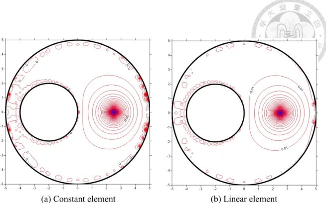
4.3 Potential contour on the plane x₃ = 0 for a concentrated source at point (2.5,0,0) using 324 nodal points and 640 triangular elements . . . 66

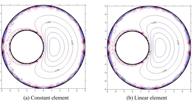
4.4 Potential contour on the plane x₃ = 0 for a concentrated source at point (2.5,0,0) with nearly singularity alleviated using 324 nodal points and 640 triangular elements . . . 66

4.5 Potential contour on the plane x₃ = 0 for a concentrated source at point (2.5,0,0) using 804 nodal points and 1600 triangular elements . . . 67

(11)

4.6 Potential contour on the plane x₃ = 0 for a concentrated source at point (2.5,0,0) with nearly singularity alleviated using 804 nodal points and

1600 triangular elements . . . 67

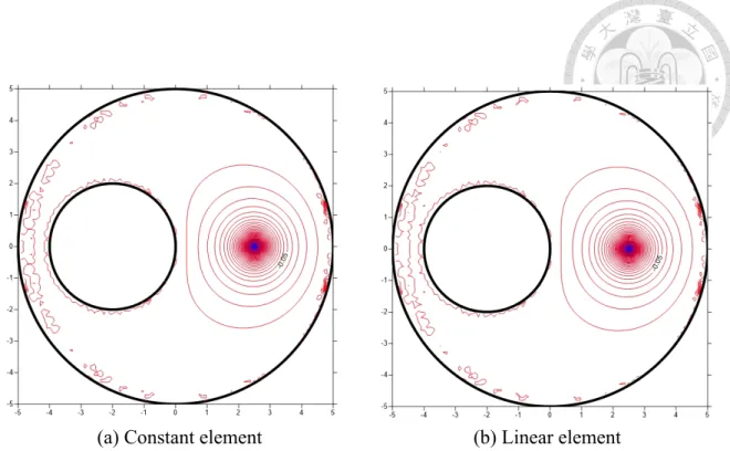
4.7 Analytical solution on the plane x3 = 0 for a concentrated source at point (2.5,0,0) using bispherical coordinates . . . 68

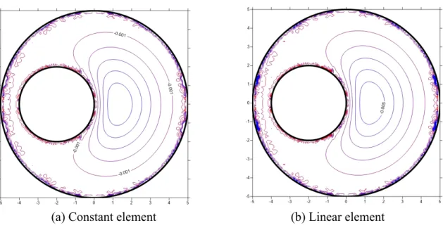
4.8 Potential contour on the plane x₃ = 0 for a concentrated source at point (0,0,2.5) using 324 nodal points and 640 triangular elements . . . 68

4.9 Potential contour on the plane x₃ = 0 for a concentrated source at point (0,0,2.5) with nearly singularity alleviated using 324 nodal points and 640 triangular elements . . . 69

4.10 Potential contour on the plane x₃ = 0 for a concentrated source at point (0,0,2.5) using 804 nodal points and 1600 triangular elements . . . 69

4.11 Potential contour on the plane x₃ = 0 for a concentrated source at point (0,0,2.5) with nearly singularity alleviated using 804 nodal points and 1600 triangular elements . . . 70

4.12 Analytical solution on the plane x₃ = 0 for a concentrated source at point (0,0,2.5) using bispherical coordinates . . . 70

4.13 Geometry and boundary conditions of a cube . . . 71

4.14 The framework of heat conduction . . . 71

4.15 Geometry of heat conduction in functionally graded material . . . 72

4.16 Temperature distribution on the plane x₂ = 0 for β = 0 . . . . 72

4.17 Temperature distribution on the plane x₂ = 0 with nearly singularity alle- viated for β = 0 . . . . 73

4.18 Exact solution of temperature distribution on the plane x₂ = 0 for β = 0 . 73 4.19 Temperature distribution on the line (x₁, 0.5, 0.5) for β = 0 . . . . 74

4.20 Temperature distribution on the plane x2 = 0 for β = 1.5 . . . . 75

4.21 Temperature distribution on the plane x₂ = 0 plane with nearly singularity alleviated for β = 1.5 . . . . 75 4.22 Exact solution of temperature distribution on the plane x₂ = 0 for β = 1.5 76

(12)

4.23 Temperature distribution on the line (x₁, 0.5, 0.5) for β = 1.5 . . . . 77

4.24 Temperature distribution on the plane x₂ = 0 for β = 10 . . . . 78

4.25 Temperature distribution on the plane x₂ = 0 plane with nearly singularity alleviated for β = 10 . . . . 78

4.26 Exact solution of temperature distribution on the plane x2 = 0 for β = 10 79 4.27 Temperature distribution on the line (x₁, 0.5, 0.5) for β = 10 . . . . 80

4.28 The framework of magnetostatics . . . 81

4.29 A magnetized sphere in an external uniform magnetic field . . . 81

4.30 Mesh distribution of triangular elements for the sphere . . . 82

4.31 Vector field (A₁, A₂) for case A on the plane x₃ = 0 . . . 82

4.32 Vector field (A₁, A₂) for case A on the plane x₃ = 0 with nearly singularity alleviated . . . 83

4.33 Exact solution of (A₁, A₂) for case A on the plane x₃ = 0 . . . 83

4.34 Distribution of A₂ on the x₁-axis for case A . . . 84

4.35 Vector field (A₁, A₂) for case B on the plane x₃ = 0 plane . . . 85

4.36 Vector field (A₁, A₂) for case B on the plane x₃ = 0 plane with nearly singularity alleviated . . . 85

4.37 Exact solution of (A₁, A₂) for case B on the plane x₃ = 0 . . . 86

4.38 Distribution of A2 on the x1-axis for case B . . . 87

4.39 Vector field (A₁, A₂) for case C on the plane x₃ = 0 . . . 88

4.40 Vector field (A₁, A₂) for case C on the plane x₃ = 0 plane with nearly singularity alleviated . . . 88

4.41 Exact solution of (A₁, A₂) for case C on the plane x₃ = 0 . . . 89

4.42 Distribution of A₂ on the x₁-axis for case C . . . 90

4.43 Vector field (A₁, A₂) for case D on the plane x₃ = 0 . . . 91

4.44 Vector field (A1, A2) for case D on the plane x3 = 0 with nearly singularity alleviated . . . 91

4.45 Exact solution of (A₁, A₂) for case D on the plane x₃ = 0 . . . 92

(13)

4.47 Vector field (B₁, B₃) for all cases on the plane x₂ = 0 . . . 94 4.48 Vector field (B₁, B₃) for all cases on the plane x₂ = 0 with nearly singu-

larity alleviated . . . 94 4.49 Exact solution of (B1, B3) for all cases on the plane x2 = 0 . . . 95 4.50 Distribution of B3on the x1-axis for all cases . . . 96 4.51 Distribution of B₃on the x₁-axis for all cases at different nodal points and

linear elements . . . 97 A.1 An arbitrary domain on the plane and the interior angle at the boundary

point y . . . 111

(14)

List of Tables

3.1 The relation amongH, Cl0,2and Cl3 . . . 42 3.2 Quaternion multiplication . . . 42 3.3 Comparsion of four kernel functions inH and R²for the 3D Laplace equation 42 3.4 Order of singularity . . . 43 3.5 Comparsion of boundary integral equations inH and R²for the 3D Laplace

equation . . . 44

(15)

Chapter 1 Introduction

1.1 Motivation and literature reviews

In some engineering problems, the associated physical phenomena such as steady state heat conduction [1, 2, 3], magentostatics [4] and potential flow [5] are modelled mathematically by the Laplace equation. By solving the mathematical models of these problems, we can simulate and predict their physical behaviour. Nowadays, researchers and engineers use such numerical methods as the finite element method (FEM), finite dif- ference method (FDM) and boundary element method (BEM) to solve engineering problems.

The FEM is versatile in dealing with almost every kind of problems and have been developed into commercial software ready for applications. They need discretization ev- erywhere in the domain. The BEM is another approach featuring discretization only on the boundary. Since only boundary discretization is required in the use of BEM, mesh reduction is an immediate benefit [6, 7, 8]. More researches paid attention on the real valued BIE and BEM [9]. Actually, complex analysis is an effective technique to solve engineering problems governed by the Laplace equation such as the torsion problem [10], the problem of plane elasticity [11] and crack problem [12].

The complex variable boundary element method (CVBEM) [13] is based on the Cauchy integral formula, residue theorem and Cauchy-Riemann equations. The real part

(16)

stream function in the two-dimensional potential flow problem, respectively. In the con- ventional CVBEM, the complex valued function must be a holomorphic function. How- ever, a complex valued harmonic function is not necessarily a holomorphic function. For this reason, Lee et al. [14] proposed a generalized CVBEM for the torsion problem. The CVBEM is limited to two-dimensional problems. Extending complex variables to quaternionic variables in order to solve three-dimensional problems is long desired. In this pro- cess, preserving some benefits of complex variable is possible. Quaternion algebra is proposed by Halmilton in 1843 [15]. Later in 1878, Clifford proposed an algebra named after him [16]. Complex algebra is a subalgebra of quaternion algebra [17]. Complex algebra and quaternion algebra can be seen as special kinds of Clifford algebras. Fueter started a series of development of quaternion analysis since 1930 [18, 19]. Now, there is a new field of quaternion analysis [20, 21, 22, 23] and Clifford analysis [24, 25, 26].

Recently, Liu and Hong used Clifford analysis to solve for general solutions of both isotropic elasticity [27] and anisotropic elasticity [28, 29]. Hong and Liu derived the quaternion valued BIE and developed the quaternion BEM to solve three-dimensional problems of magnetostatics [30] and elasticity [28, 29]. Hong et al. [31], Lin [32] and Lee [33] have done similar works for Clifford valued BIEs and BEM. In this thesis, we focus on developing and applying the quaternion BEMs to the three three-dimensional problems: Green’s function in a medium between eccentric spheres, heat conduction in functionally graded materials and magnetostatic problems.

1.2 Scope and organization of the thesis

In the thesis, we solve three engineering problems governed by three-dimensional Laplace equation in quaternionic variable. The thesis is organized as follows.

Chapter 2 revisits the real valued BIEs for the boundary, domain and out-of-domain points by using Green’s third identity in three-dimensional space. Derived are not only the BIEs but also the normal derivative of BIEs. It is noted that our BIE formulations are suitable for both smooth and non-smooth boundaries.

(17)

gebra and derive quaternion valued BIEs for the boundary, domain and out-of-domain points in the three-dimensional space. Moreover, we also derive the Dirac derivative of quaternion valued BIEs. Regarding the exterior problem, a constraint decay condition at infinity has been found. We also prove commutativity by using different routes to derive the Dirac derivative quaternion valued singular BIE. We discretize the quaternion valued BIE by using the constant elements and linear elements. Before discretizing the BIE, we can analytically evaluate the Cauchy principal value (CPV) by using a simple quaternion valued harmonic function. In a similar way, we evaluate the nearly singular integral equation for the points very close to the boundary, thus overcoming the phenomenon of the boundary layer effect due to the nearly singular integral.

Chapter 4 uses a quaternion valued BEM to solve the problem of Green’s function for a bounded domain [34], heat conduction in functionally graded materials [35] and magnetostatic problems [36]. Both constant element and linear element are used to demonstrate the validity of present approach.

Finally, we state our conclusions and propose several future researches in the last chapter.

(18)

Chapter 2 Dual BIEs in R ³

In this chapter, we revisit real variable dual boundary integral equations (BIEs) for the three-dimensional Laplace equation in real variable. First, according to Green’s second identity, we derive the real variable BIEs. Then, we apply normal derivative to the BIEs to obtain the normal derivative of BIEs. These BIEs are established for the collocation point y at any position, and not only for the smooth boundary, but also for the non-smooth boundary.

When the collocation point is on the boundary, the BIE encounters singularity but it is proved that the singular integral exists in sense of the Cauchy principal value, and the normal derivative of BIE encounters singularity and hypersingularity but it is proved that the singular integral exists in sense of the Cauchy principal value and that the hypersingular exists in sense of Hadamard principal value.

2.1 Real valued BIEs

We consider an open and simply connected domain Ω⊂ R³bounded by the boundary

∂Ω in three-dimensional Euclidean spaceR³. Three dimensional Laplace equation is

− ∆f(x) = 0, ∀x ∈ Ω, (2.1)

(19)

where f (x) is a real valued function, x = (x₁, x₂, x₃) is the coordinates of the field point x in the domain Ω and ∆ is the three-dimensional Laplace operator which is ∆ = _∂x^∂²2

1 +

∂²

∂x²₂ +_∂x^∂²2

3 in the Cartesian coordinates.

The fundamental solution is

U (x− y) = 1

4π|r|, (2.2)

which by definition satisfies

− ∆U(x − y) = δ(x − y), ∀x, y ⊂ R³. (2.3)

The δ(x− y) is the Dirac-delta function and y = (y1, y₂, y₃) is a source point. r = (r1, r2, r3) = x− y is from y to x and |r| ≡ |x − y| is the distance between the field point x and the source point y. Green’s second identity is

∫

Ω

(Φ∆Ψ− Ψ∆Φ)d³x =

∫

∂Ω

(Φ∂Ψ

∂n − Ψ∂Φ

∂n)dS(x). (2.4)

Substituting Φ = U (x− y) and Ψ = f(x) in Green’s second identity, we obtain

∫

Ω

f (x)δ(x− y)d³x =

∫

∂Ω

[U (x− y)∂f (x)

∂n(x) − f(x)∂U (x− y)

∂n(x) ]dS(x), (2.5)

where _∂n(x)^∂ = n_i(x)_∂x^∂

i is the operator of normal derivative. Hence, the singular kernel function ^{∂U (x}_∂n(x)^−y) can be written as

∂U (x− y)

∂n(x) =−r_in_i(x)

4π|r|³ , (2.6)

where n(x) = (n1, n2, n3) in the right-hand side is the outward unit normal vector.

When y is in the domain ( y∈ Ω ) , Eq. (2.5) becomes

f (y) =

∫

∂Ω

[U (x− y)∂f (x)

∂n(x) − f(x)∂U (x− y)

∂n(x) ]dS(x), y ∈ Ω. (2.7)

(20)

If the points y is out of the domain ( y∈ R³\ clΩ ) , Eq. (2.5) becomes

0 =

∫

∂Ω

[U (x− y)∂f (x)

∂n(x) − f(x)∂U (x− y)

∂n(x) ]dS(x), y ∈ R³\ clΩ, (2.8)

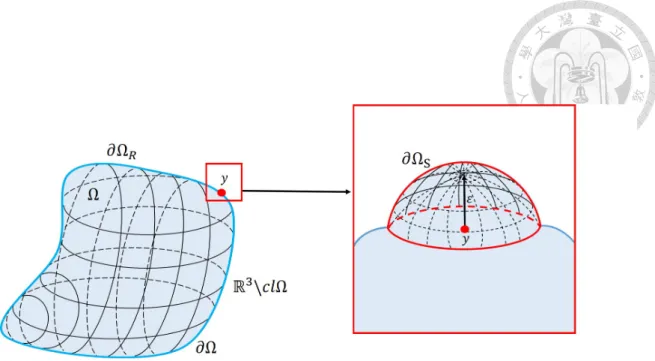
where clΩ denotes the closure of Ω, that is Ω∪∂Ω. If y is located on the boundary (y ∈ ∂Ω), the integral in Eq. (2.5) may encounter the singularity problem. We use the concept of the bump contour to calculate the free term. There is a simply connected domain as shown in Fig. 2.1. Then, the boundary is divided into two parts ∂Ω\clB³(y, ε) and S²(y, ε)∩ clΩ as shown in Fig. 2.2, so is the boundary integral

∫

∂Ω

· · · dS(x) = lim

ε→0

∫

∂Ω\clB³(y,ε)

· · · dS(x) + lim

ε→0

∫

S²(y,ε)∩clΩ· · · dS(x), (2.9) where B³(y, ε) is a ball which center is y and radius is ε and S²(y, ε) is the surface of the sphere inR³. We use the symbol ∂ΩRand ∂ΩSto denote ∂Ω\clB³(y, ε) and S²(y, ε)∩clΩ.

Therefore, we can rewrite Eq. (2.9) as

∫

∂Ω

· · · dS(x) = lim

ε→0

∫

∂ΩR

· · · dS(x) + lim

ε→0

∫

∂ΩS

· · · dS(x). (2.10)

Then, Eq. (2.8) becomes

0 = lim

ε→0

∫

∂ΩR+∂ΩS

[U (x− y)∂f (x)

∂n(x) − f(x)∂U (x− y)

∂n(x) ]dS(x). (2.11)

The first term on the right-hand side of Eq. (2.11) can be written as

limε→0

∫

∂ΩR+∂ΩS

U (x− y)∂f (x)

∂n(x)dS(x) = lim

ε→0

∫

∂ΩR

U (x− y)∂f (x)

∂n(x)dS(x) + lim

ε→0

∫

∂ΩS

U (x− y)∂f (x)

∂n(x)dS(x).

(2.12)

When ε tends to zero, the first term on the right-hand side of Eq. (2.12) does not go to infinity and the second term vanishes, so that the first term has no singularity problem.

(21)

Therefore, Eq. (2.12) becomes

ε→0lim

∫

∂Ω

U (x− y)∂f (x)

ε→0

∫

∂ΩR

U (x− y)∂f (x)

ε→0

∫

∂ΩS

1 4πε

∂f (x)

∂n(x)ε²dA(x)

= lim

ε→0

∫

∂Ω_R

U (x− y)∂f (x)

∂n(x)dS(x).

(2.13)

The second term on the right-hand side of Eq. (2.11) can be written as

limε→0

∫

∂ΩR+∂ΩS

∂U (x− y)

∂n(x) f (x)dS(x) = lim

ε→0

∫

∂ΩR

∂U (x− y)

∂n(x) f (x)dS(x) + lim

ε→0

∫

∂ΩS

∂U (x− y)

∂n(x) f (x)dS(x).

(2.14)

The first term on the right-hand side of Eq. (2.14) seems to encounter the singular integral;

however, the punctured integral exists in the sense of the Cauchy principal value:

εlim→0

∫

∂ΩR

∂U (x− y)

∂n(x) f (x)dS(x) =−

∫

∂Ω

∂U (x− y)

∂n(x) f (x)dS(x), (2.15)

where∫−

denotes the Cauchy principal value (CPV) [37].¹ The second term on the right- hand side of Eq. (2.14) is

limε→0

∫

∂ΩS

∂U (x− y)

∂n(x) f (x)dS(x)

= lim

ε→0

∫

∂ΩS

−εni(x)n_i(x)

4πε³ f (x)ε²dA(x)

=− lim

ε→0

∫

∂ΩS

1

4π[f (y) + (−εn(x) · ∇yf (y)) + H.O.T.)]dA(x)

=− lim

ε→0

∫

∂ΩS

f (y) 4π dA(x)

=− αf (y) 4π ,

(2.16)

where α is the solid angle subtended in the interior side at the boundary point y and H.O.T.

1Recall that the definition of CPV in one dimension is

−

∫ b a

1 s− cds =

∫ c−ε a

1 s− cds +

∫ b c+η

1 s− cds,

(22)

stands for the higher order terms. Combining Eq. (2.15) with Eq. (2.16), we obtain

∫

∂Ω

∂U (x− y)

∂n(x) f (x)dS(x) =−

∫

∂Ω

∂U (x− y)

∂n(x) f (x)dS(x)− αf (y)

4π . (2.17)

After arranging Eqs. (2.13) and (2.17), we obtain the real variable singular BIE when the source point is located on the boundary,

αf (y) 4π =

∫

∂Ω

U (x− y)∂f (x)

∂n(x)dS(x)− −

∫

∂Ω

∂U (x− y)

∂n(x) f (x)dS(x), y ∈ Ω. (2.18)

In summary, real variable BIE can be rewritten as

c(y)f (y) =

∫

∂Ω

U (x− y)t(x)dS(x) −

∫ (y)

∂Ω

T (x− y)f(x)dS(x), (2.19)

where t(x) = ^{∂f (x)}_∂n(x), T (x− y) = ^{∂U (x}_∂n(x)^−y),

c(y) =











1 ∀y ∈ Ω, α

4π ∀y ∈ ∂Ω, 0 ∀y ∈ R³\ clΩ,

and

∫ (y)

∂Ω

=











∫

∂Ω

∀y ∈ Ω,

−

∫

∂Ω

∀y ∈ ∂Ω,

∫

∂Ω

∀y ∈ R³\ clΩ.

(2.20)

2.2 Normal derivative of real valued BIEs

In this section, we are going to derive the normal derivative of BIEs. We apply the normal derivative operator (_∂n(y)^∂ ) at point y to Eq. (2.7). Thus, the results are

∂f (y)

∂n(y) =

∫

∂Ω

[∂U (x− y)

∂n(y)

∂f (x)

∂n(x) − f(x)∂²U (x− y)

∂n(x)∂n(y)]dS(x), y ∈ Ω; (2.21)

and

0 =

∫

∂Ω

[∂U (x− y)

∂n(y)

∂f (x)

∂n(x) − f(x)∂²U (x− y)

∂n(x)∂n(y)]dS(x), y ∈ R³\ clΩ. (2.22)

(23)

into two parts. Thus from Eq. (2.10),

0 = lim

ε→0

∫

∂ΩR+∂ΩS

[∂U (x− y)

∂n(y)

∂f (x)

∂n(x) − f(x)∂²U (x− y)

∂n(x)∂n(y)]dS(x), (2.23)

where

∂U (x− y)

∂n(y) = (x_i − yi)n_i(y)

4π|x − y|³ , (2.24)

and

∂²U (x− y)

∂n(x)∂n(y) =−3(xi− yi)(xj − yj)ni(x)nj(y)

4π|x − y|⁵ +ni(x)ni(y)

4π|x − y|³. (2.25) We examine Eq. (2.23) as follows. For the part over ∂Ω_R of the first term on the right-hand side of Eq. (2.23), the Cauchy principal value (CPV) exists when ε tends to zero.

limε→0

∫

∂ΩR

∂U (x− y)

∂n(y)

∂f (x)

∂n(x)dS(x) =−

∫

∂Ω

∂U (x− y)

∂n(y)

∂f (x)

∂n(x)dS(x). (2.26)

The part over ∂ΩScan be written

limε→0

∫

∂Ω_S

∂U (x− y)

∂n(y)

∂f (x)

ε→0

∫

∂Ω_S

(x_i− yi)n_i(y) 4π|ε|³

∂f (x)

∂n(x)dS(x)

= lim

ε→0

∫

∂ΩS

−εni(x)n_i(y) 4π|ε|³

∂f (x)

∂x_j

x=yn_j(x)ε²dA(x)

= lim

ε→0

∫

∂ΩS

−ni(x)ni(y) 4π

∂f (x)

∂x_j

x=ynj(x)dA(x).

(2.27) where ^{∂f (x)}_∂n(x) has the Taylor series expansion

∂f (x)

∂n(x)

=∂f (y)

∂x₁ n₁(x) + ∂f (y)

∂x₂ n₂(x) + ∂f (y)

∂x₃ n₃(x) +∂f (x)

∂x₁

x=y

(x₁− y1)

∂x₁ n₁(x) + ∂f (x)

∂x₂

x=y

(x₂− y2)

∂x₂ n₂(x) + ∂f (x)

∂x₃

x=y

(x₃− y3)

∂x₃ n₃(x)

=∂f (x)

∂x₁

x=y

n₁(x) + ∂f (x)

∂x₂

x=y

n₂(x) + ∂f (x)

∂x₃

x=y

n₃(x)

=∂f (x)

∂x_i

x=yni(x).

(2.28)

(24)

Upon combining Eqs. (2.26) and (2.27), the first term on the right-hand side of Eq. (2.23) becomes

∫

∂Ω

∂U (x− y)

∂n(y)

∂f (x)

∂n(x)dS(x) =−

∫

∂Ω

∂U (x− y)

∂n(y)

∂f (x)

ε→0

∫

∂ΩS

−ni(x)n_i(y) 4π

∂f (x)

∂xj

x=y

n_j(x)dA(x).

(2.29)

For the part over ∂Ω_Sof the second integral term on the right-hand side of Eq. (2.23), the normal derivative of the kernel and density function become

∂²U (x− y)

∂n(x)∂n(y) =−3(x_i− yi)(x_j− yj)n_i(x)n_j(y)

4π|x − y|⁵ +n_i(x)n_i(y) 4π|x − y|³

=−3(−εni(x))(−εnj(x))ni(x)nj(y)

4πε⁵ +ni(x)ni(y) 4πε³

=−3n_j(x)n_j(y)

4πε³ +n_i(x)n_i(y) 4πε³

=−3n_i(x)n_i(y)

4πε³ +n_i(x)n_i(y)

4πε³ =−n_i(x)n_i(y) 2πε³ ,

(2.30)

and

f (x) = f (y) + ∂f (x)

∂x₁

x=y(x1− y1) + ∂f (x)

∂x₂

x=y(x2− y2) + ∂f (x)

∂x₃

x=y

(x₃− y3) + H.O.T.

= f (y)− ∂f (x)

∂x_i

x=y(εn_i(x)),

(2.31)

respectively. Therefore, the part over ∂Ω_S becomes

εlim→0

∫

∂Ω_S

∂²U (x− y)

∂n(x)∂n(y)f (x)dS(x)

= lim

ε→0

∫

∂ΩS

[−n_i(x)n_i(y)

2πε³ (f (y)− ∂f (x)

∂x_j

x=yεn_j(x))]dS(x)

= lim

ε→0

∫

∂ΩS

[−ni(x)ni(y)

2πε f (y) + ni(x)ni(y) 2π

∂f (x)

∂x_j

x=ynj(x)]dA(x).

(2.32)

Second, we deal with the part over ∂Ω_Rof the second term on the right-hand side of Eq.

(25)

(2.23). It can be written as follows:

limε→0−

∫

∂ΩR

∂²U (x− y)

∂n(x)∂n(y)f (x)dS(x) = lim

ε→0−

∫

∂ΩR

∂²U (x− y)

∂n(x)∂n(y)[f (x)− f(y)]dS(x) + lim

ε→0−

∫

∂ΩR

∂²U (x− y)

∂n(x)∂n(y)f (y)dS(x).

(2.33)

From Eq. (2.22), we can let f (x) be a constant, and obtain

0 =− lim

ε→0−

∫

∂ΩR

∂²U (x− y)

∂n(x)∂n(y)dS(x)− lim

ε→0

∫

∂ΩS

∂²U (x− y)

∂n(x)∂n(y)dS(x). (2.34)

Substituting Eq. (2.30) into Eq. (2.34), we obtain

limε→0−

∫

∂ΩR

∂²U (x− y)

∂n(x)∂n(y)dS(x) =− lim

ε→0

∫

∂ΩS

∂²U (x− y)

∂n(x)∂n(y)dS(x)

= lim

ε→0

∫

∂ΩS

n_i(x)n_i(y)

2πε³ dS(x) = lim

ε→0

∫

∂ΩS

n_i(x)n_i(y)

2πε dA(x).

(2.35)

When ε tends to zero, the first term on the right-hand side of Eq. (2.33) exists in the sense of the Hadamard principal value (HPV) [38].

limε→0−

∫

∂ΩR

∂²U (x− y)

∂n(x)∂n(y)[f (x)− f(y)]dS(x) = =

∫

∂Ω

∂²U (x− y)

∂n(x)∂n(y)f (x)dS(x), (2.36)

where∫⁼

is HPV.² Arranging Eq. (2.33) to Eq. (2.36), we have

∫

∂Ω

∂²U (x− y)

∂n(x)∂n(y)f (x)dS(x) = lim

ε→0−

∫

∂Ω_R

∂²U (x− y)

∂n(x)∂n(y)[f (x)− f(y)]dS(x) + lim

ε→0−

∫

∂ΩR

∂²U (x− y)

∂n(x)∂n(y)f (y)dS(x) + lim

ε→0

∫

∂ΩS

∂²U (x− y)

∂n(x)∂n(y)f (x)dS(x)

= =

∫

∂Ω

∂²U (x− y)

∂n(x)∂n(y)f (x)dS(x) + lim

ε→0

∫

∂Ω_S

n_i(x)n_i(y) 2π

∂u(x)

∂x_j

x=y

(n_j(x))dA(x).

(2.37)

Finally, combining Eq. (2.29) and (2.37), we obtain the normal derivative of singular

2Recall that the definition of the HPV in one dimension is

=

∫ b a

f (s)ds = lim

ε→0,η→0[−

∫ c−ε a

f (s)ds +−

∫ b c+η

f (s)ds],

where f (s)’s order is ¹ and ε = η.

(26)

BIE

limε→0

∫

∂Ω_S

3n_i(x)n_i(y)

4π t(x)dA(x)

=−

∫

∂Ω

∂U (x− y)

∂n(x)

∂f (x)

∂n(x)dS(x)− =

∫

∂Ω

∂²U (x− y)

∂n(x)∂n(y)f (x)dS(x).

(2.38)

Let

L(x− y) = ∂U (x− y)

∂n(x) , (2.39)

M (x− y) = ∂²U (x− y)

∂n(x)∂n(y), (2.40)

t(x) = ∂f (x)

∂n(x). (2.41)

Then, the normal derivative of BIEs are written

h(y)f (y) =

∫ (y1)

∂Ω

L(x− y)t(x)dS(x) −

∫ (y2)

∂Ω

M (x− y)f(x)]dS(x) (2.42)

where

h(y) =











∂

∂n(y) ∀y ∈ Ω,

εlim→0

∫

∂ΩS

[3n_i(x)n_i(y) 4π

∂

∂xj|x=yn_j(x)]dA(x)∀y ∈ ∂Ω, 0∀y ∈ R³\ clΩ,

(2.43)

∫ _(y₁₎

∂Ω

=











∫

∂Ω

∀y ∈ Ω,

−

∫

∂Ω

∀y ∈ ∂Ω,

∫

∂Ω

∀y ∈ R³\ clΩ, and

∫ _(y₂₎

∂Ω

=











∫

∂Ω

∀y ∈ Ω,

=

∫

∂Ω

∀y ∈ ∂Ω,

∫

∂Ω

∀y ∈ R³\ clΩ.

(2.44)

(27)

Figure 2.1: The simply connected domain inR³

Figure 2.2: The boundary ∂Ω_Rand ∂Ω_S

(28)

Chapter 3 Quaternion valued BIEs in R ³

In this chapter, we derive the quaternion valued BIEs. First, we introduce quaternion algebra and analysis. Then, according to quaternion valued Stokes’ theorem, we derive the quaternion valued BIEs for the three-dimensional Laplace equation in quaternionic variable. When the source point is located on the boundary, an encounter with the singularity problem lead us to prove that the singular integral exists in the sense of the Cauchy principal value (CPV). For this, we analytically evaluate the CPV by introducing a simple quaternion valued harmonic function. In addition, when the source point is close to the boundary, it is present a nearly singular phenomenon. We also alleviate this problem by analytically evaluating the nearly singular integral. Finally, we discretize the quaternion valued BIEs into the quaternion BEM by considering both constant element and linear element.

The derivation of the BIEs for a point on the boundary may be achieved by integrat- ing over the interior or exterior bump detours or even cutting direct across the point of singularity. Furthermore, we prove the commutativity of the Dirac operator and the trace operator. We not only derive the BIE for the interior problem, but also derive it for the exterior problem. The unit outward normal vector and the ordinary surface element are combined into the quaternion valued oriented surface element.

(29)

3.1 Quaternion algebra and analysis

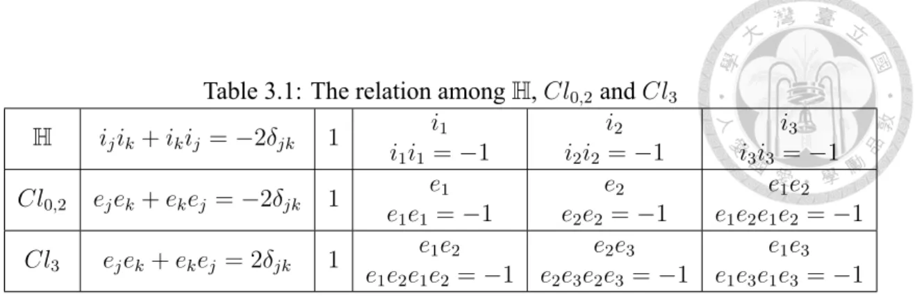
In this section, we introduce quaternion algebra. Quaternion algebra is isomorphic to Clifford algebra Cl_0,2or the even subalgebra of Cl₃. The relation amongH, Cl0,2and Cl₃are summarized in Table 3.1. Quaternion algebra has four basis elements:

1, i1, i2, i3. (3.1)

The quaternion product i_ji_kof i_j and i_kis defined by the quaternion product rule and the multiplication is shown in Table 3.2.

i_ji_k+ i_ki_j =−2δjk, j, k = 1, 2, 3. (3.2)

A quaternion number or simply a quaternion is

a = a01 + a1i1+ a2i2+ a3i3, a∈ H, ai ∈ R. (3.3)

The conjugate a is

a = a₀1− a1i₁− a2i₂− a3i₃, a∈ H, ai ∈ R. (3.4)

In quaternion algebra, a point arbitrarily located in three-dimensional space may be ex- pressed as

x =

∑3 j=1

x_ji_j, x∈ H, xi ∈ R. (3.5)

For a quaternion valued function, we can define a function in the Euclidean spaceR³ as

f (x) :R³ → H, (3.6)

where

f (x) = f₀(x) +

∑3 j=1

f_j(x)i_j, (3.7)

(30)

andH, respectively. In general, the multiplication of quaternions are non-commutative.

For example, the multiplication of two quaternions

a = 1 + 2i₁+ 4i₂, b = 1 + 2i₃.

(3.8)

Let a multiple by b and b multiple by a, the results are

ab = 1 + 10i₁+ 2i₃, ba = 1− 6i1+ 8i₂+ 2i₃.

(3.9)

Obviously, ab is not equal to ba.

In Cartesian coordinates, the Dirac (Fueter) operator inH is defined as

D(x) = i1

∂

∂x₁ + i2

∂

∂x₂ + i3

∂

∂x₃ (3.10)

and the conjugate D(x) is

D(x) = −D(x) = −i1

∂

∂x₁ − i2

∂

∂x₂ − i3

∂

∂x₃. (3.11)

The three-dimensional Laplace operator is

∆ =−D(x)D(x) = D(x)D(x). (3.12)

The fundamental solution of the three-dimensional Laplace equation is

U (x− y) = 1

4π|x − y|, (3.13)

where the fundamental solution U (x− y) satisfies

− ∆U(x − y) = δ(x − y), (3.14)

(31)

in which δ(x− y) is the Dirac delta function and y is the source point.

3.2 Quaternion valued BIEs

Quaternion valued Stokes’ theorem in three-dimensional space is

∫

∂Ω

g(x)n(x)h(x)dS(x) =

∫

Ω

[(g(x)D(x))h(x) + g(x)(D(x)h(x))]d³x, (3.15)

where g(x), h(x) and n(x) are quaternion valued functions and n(x) = ∑3

j=1n_j(x)i_j is the outward unit vector normal to the boundary. We will derive the quaternion valued BIE for quaternion valued Laplace equation in three dimensions based on Stokes’ theorem (3.15).

Let g(x) = U (x− y)D(x) and h(x) = f(x); Eq. (3.15) becomes

∫

∂Ω

U (x− y)D(x)n(x)f(x)dS(x)

=

∫

Ω

[(U (x− y)D(x)D(x))f(x) + D(x)U(x − y)(D(x)f(x))]d³x.

(3.16)

We can also let g(x) = U (x− y) and h(x) = −D(x)f(x); Eq. (3.15) becomes

∫

∂Ω

−U(x − y)n(x)D(x)f(x)dS(x)

=

∫

Ω

[U (x− y)D(x)(−D(x)f(x)) − U(x − y)(D(x)D(x)f(x))]d³x.

(3.17)

Combining Eq.(3.16) with Eq. (3.17), we have

∫

∂Ω

−C(x − y)n(x)f(x)dS +

∫

∂Ω

U (x− y)n(x)D(x)f(x)dS

=

∫

Ω

[(U (x− y)D(x)D(x))f(x) − U(x − y)(D(x)D(x)f(x))]d³x,

(3.18)

where the Cauchy kernel is

C(x− y) = D(x)U(x − y) = (x− y)

4π|x − y|³. (3.19)

(32)

When f (x) is a quaternion valued harmonic function, D(x)D(x)f (x) is equal to zero.

Then, Eq. (3.18) can be written as

∫

Ω

δ(x−y)f(x)d³x =

∫

∂Ω

U (x−y)n(x)D(x)f(x)dS(x)−

∫

∂Ω

C(x−y)n(x)f(x)dS(x).

(3.20) When the point y is in the domain and out of domain, the quaternion valued BIEs are

f (y) =

∫

∂Ω

U (x− y)n(x)D(x)f(x)dS −

∫

∂Ω

C(x− y)n(x)f(x)dS, y ∈ Ω, (3.21)

and

0 =

∫

∂Ω

U (x− y)n(x)D(x)f(x)dS −

∫

∂Ω

C(x− y)n(x)f(x)dS, y ∈ R³\ clΩ, (3.22)

respectively. When the source point y is on the boundary, an encounter with the singular integral leads us to use the interior bump detour to deal with this problem. We divide the boundary into two parts

∂Ω = ∂Ω\clB³(y, ε) + S²(y, ε)∩ clΩ. (3.23)

The sketches of ∂Ω\clB³(y, ε) and S²(y, ε)∩ clΩ are shown in Fig. 2.2. Then, we can use the symbol ∂Ω_R and ∂Ω_S to denote ∂Ω\clB³(y, ε) and S²(y, ε)∩ clΩ, respectively.

The original integral symbol is

∫

∂Ω

· · · dS(x) = lim

ε→0

∫

∂Ω\clB³(y,ε)

· · · dS(x) + lim

ε→0

∫

S²(y,ε)∩clΩ· · · dS(x). (3.24) Therefore, we can rewrite as

∫

∂Ω

· · · dS(x) = lim

ε→0

∫

∂ΩR

· · · dS(x) + lim

ε→0

∫

∂ΩS

· · · dS(x). (3.25)

(33)

Using Eq. (3.25), we rewrite Eq. (3.22) as

0 = lim

ε→0

∫

∂ΩR+∂ΩS

U (x−y)n(x)D(x)f(x)dS(x)+lim

ε→0

∫

∂ΩR+∂ΩS

C(x−y)n(x)f(x)dS(x).

(3.26) The first term on the right-hand side of Eq. (3.26) has no singularity and is derive as follows:

∫

∂ΩR+∂ΩS

U (x− y)n(x)D(x)f(x)dS(x)

= lim

ε→0

∫

∂ΩR

U (x− y)n(x)D(x)f(x)dS(x) + lim

ε→0

∫

∂ΩS

U (x− y)n(x)D(x)f(x)dS(x)

= lim

ε→0

∫

∂ΩR

U (x− y)n(x)D(x)f(x)dS(x) + lim

ε→0

∫

∂ΩS

1

4π|ε|n(x)D(x)f (x)ε²dA(x)

= lim

ε→0

∫

∂ΩR

U (x− y)n(x)D(x)f(x)dS(x).

(3.27) The part over ∂ΩRof the second term on the right-hand side of Eq. (3.26) exists in the sense of the Cauchy principal value (CPV),

εlim→0

∫

∂ΩR

C(x− y)n(x)f(x)dS(x) = −

∫

∂Ω

C(x− y)n(x)f(x)dS(x), (3.28)

where∫−

denotes the CPV. The part over ∂Ω_S of the second term on the right-hand side of Eq. (3.26) is

εlim→0

∫

∂ΩS

C(x− y)n(x)f(x)dS(x)

= lim

ε→0

∫

∂ΩS

(x− y)n(x)

4π|ε|³ f (x)dS(x) = lim

ε→0

∫

∂ΩS

−εn(x)n(x)

4π|ε|³ f (x)ε²dA(x)

= lim

ε→0

∫

∂ΩS

1

4π{[f(x) − f(y)] + f(y)}dA(x) = lim

ε→0

∫

∂ΩS

f (y) 4π dA(x)

=αf (y) 4π ,

(3.29)

(34)

where α is the solid angle subtended in the interior side at the boundary point y and











x− y = −εn(x), (n(x))² =−1,

∫

∂ΩS

dS(x) = ε²α, limε→0

∫

∂ΩS

1

ε²[f (x)− f(y)]dS(x) = 0.

(3.30)

Combining Eqs. (3.27) and (3.28) with Eq. (3.29), we obtain

α

4πf (y) =

∫

∂Ω

U (x− y)n(x)D(x)f(x)dS(x) − −

∫

∂Ω

C(x− y)n(x)f(x)dS(x), y ∈ ∂Ω.

(3.31) According to the location of source point y, we have the quaternion valued BIEs

c(y)f (y) =

∫ _(y)

∂Ω

C(x−y)n(x)f(x)dS(x)−

∫ _(y)

∂Ω

U (x−y)n(x)D(x)f(x)dS(x), (3.32)

where

c(y) =











1 ∀y ∈ Ω, α

4π ∀y ∈ ∂Ω, 0 ∀y ∈ R³\ clΩ,

and

∫ (y)

∂Ω

=











∫

∂Ω

∀y ∈ Ω,

−

∫

∂Ω

∀y ∈ ∂Ω,

∫

∂Ω

∀y ∈ R³\ clΩ.

(3.33)

The above derivation was based on an integration over the interior bump detour. In fact, an integration over the exterior bump detour or a direct cutting-across integration can lead to the same quaternion valued singular BIE, as will be elaborated in the following two subsections, respectively.