不動產經紀人員所得之決定 -個人條件、加盟與直營之影響

全文

(1)國立屏東大學不動產經營學系碩士班碩士論文. 指導教授:李春長博士董呈煌博士. 不動產經紀人員所得之決定 -個人條件、加盟與直營之影響. 研究生:李育衡撰. 中華民國一百零四年六月.

(2)

(3) Acknowledgement The last time I had a student ID was 32 years ago, so I had mixed feelings about returning this one. My friends always teased me asking, “What’s the point of all this work if it won’t even get you a raise?” and I just smiled silently. This diploma is a present for my father’s 83rd birthday. He always hoped that I earn a master’s degree and thankfully I was able to fulfill his expectation. Before the program started I had already decided to be a perfect student with a perfect attendance. And I did it. Our class representative Hui-ya wondered why I wanted to buy this master’s gown. I want to hang it in my son Chun-i’s and my daughter Ssu-chia’s rooms every other night. I want them to know that their father really took these past two years seriously. Where others might see nothing more than a piece of paper, to me this is priceless. I would like to thank Professor Chun-chang Lee who is not only my teacher but also my friend. Thank you for always spending extra time instructing Yang-tung, Chien-cheng and me. I know that we are the students who were taught the most but absorbed the least. To my surprise, I finished this master’s thesis in English. It was all because of Professor Lee’s help. Thank you for all the inspiration and instruction over the past ten months. Even though the work was hard, the fruits of our labor taste sweet and rewarding. I am so grateful to have a great teacher like Professor Lee. I would also like to thank Tung-Tung, the last classmate I will ever have; thank you for everything these past two years. I will never forget you. Thanks to Professor Cheng-huang, Professor Hsin-li, and Professor Yun-ling for all the encouragement and support while writing my thesis. Thanks to Professor Ming-tsan Chen and Professor Chih-min Liang for the suggestions made during my oral defense. Thank you to my cousin Jui-yu and brother Wei-chieh for your support. And to Yu-chien, Feng-wen, Chia-yu, Shu-ming, Che-chang, Yu-hsin, Hsiao-yung, Hui-chuan for making me feel young again. Finally, I would like to thank my wife Chiung-i for her unconditional support. Over these two years, you were busy at work and at home. Thank you for supporting me in getting this degree. Don’t worry; these past two years have given me a newfound energy so I can work for another fifteen years. Thank you all once again my teachers, classmates, colleagues, relatives, and friends who assisted and accompanied me.. Yu-Heng Lee National Pingtung University Department of Real Estate Management July 2015 i.

(4) 不動產經紀人員所得之決定 -個人條件、加盟與直營之影響摘. 要. 本研究目的在於探討影響不動產經紀人員所得的因素，應用階層線性模型，以高雄市房屋仲介業經紀人員為分析對象。針對大型連鎖房屋仲介發放 510 份問卷，其中，回收 54 個分店共 319 份有效問卷，有效回收率為 62.55%。實證結果顯示，個人所得於各分店間存在著顯著差異。個人所得有 4.8%的變異是由於分店間的差異所造成。經紀人員的個人所得會受到個人層次因素，如年齡、工作時數、工作經驗的顯著影響。教育水準、年齡、工作時數與工作經驗對經紀人員所得之邊際影響效果會受到加盟與直營型態之干擾。另外，分店所在區位會直接顯著正向影響經紀人員之所得。. 關鍵字：不動產經紀人員、所得、加盟、直營、階層線性模型. ii.

(5) Factors Determining Income among Real Estate Salespersons: The Impacts of Individual Conditions, Franchises, and Regular Chains. Abstract This study explores the factors that affect the incomes of real estate salespersons by applying hierarchical linear modeling (HLM) to investigate the incomes of real estate salespersons in Kaohsiung. A total of 510 questionnaires were distributed to large chain housing agencies, of which a total of 319 effective samples were retrieved from 54 branch stores, for an effective return rate of 62.55%. The empirical results showed that individual incomes vary significantly from store to store. About 4.8% of the variation in individual incomes was due to differences among different branch stores. The individual income of a real estate salesperson is also significantly affected by individual-level factors such as age, working hours, and working experience. The marginal impact of education level, age, working hours, and working experience on real estate salesperson income is moderated by the type of store at which the given salesperson works. In addition, a branch store’s location has a direct, significant, and positive impact on a real estate salesperson’s income.. Keywords: real estate salesperson, income, franchises , regular chains, hierarchical linear modeling (HLM).. iii.

(6) Table of Contents Acknowledgements ............................................................................................... i Abstract(Chinese) .................................................................................................. ii Abstract .....................................................................................................................iii Table of Contents ................................................................................................. iv List of Figures ......................................................................................................... v List of Tables .......................................................................................................... vi 1. Introduction ......................................................................................................... 1 1.1 Research motivation and purpose ...................................................................... 1 1.2 Research process ................................................................................................ 2. 2. Literature review .............................................................................................. 4 2.1 The impact of the individual conditions on the income ..................................... 4 2.2 The impact of the branch location and management type on the income.......... 7. 3. Research method ........................................................................................... .10 3.1 Research framework ........................................................................................ 10 3.2 Empirical model settings ................................................................................. 11 3.2.1 Null model ............................................................................................. 12 3.2.2 Intercepts-as-outcomes model ............................................................... 13 3.2.3 Intercepts-and-slopes-as-outcomes model ............................................. 15 3.3 Variable setting ................................................................................................ 16. 4. Data source and sample descriptive statistics .................................. 25 4.1 Data collection ................................................................................................. 25 4.2 Sample descriptive statistics ............................................................................ 25. 5. Empirical result analysis ............................................................................ 28 5.1 Null model ....................................................................................................... 28 5.2 Intercepts-as-outcomes model ......................................................................... 29 5.3 Intercepts-and-slopes-as-outcomes .................................................................. 33. 6. Conclusion and suggestions ...................................................................... 40 6.1 Conclusion ....................................................................................................... 40 6.2 Implications ..................................................................................................... 42 6.3 Future studies ................................................................................................... 43. References ............................................................................................................... 44 Appendixes ............................................................................................................. 50 iv.

(7) List of figures Figure 1 Research process. ............................................................................................. 3 Figure 2 Research framework. .................................................................................. …11. v.

(8) List of Tables Table 1 Variable descriptions and definitions. ............................................................. 23 Table 2 Individual-level descriptive statistics (N=319). ............................................... 27 Table 3 Branch-level descriptive statistics (N=54). ...................................................... 28 Table 4 Empirical results of null model and intercepts-as-outcomes model ................ 37 Table 5 Empirical results of intercepts-and-slopes-as- outcomes model...................... 38. vi.

(9) 1. Introduction 1.1 Research motivation and purpose The industrial characteristics and work patterns of the housing agency industry are different from those of other general industries. In addition to longer working hours, the management types used in the industry are also different from those used in other industries. These differences may result in differences in individual income performance. In recent years, research on the incomes of housing agency employees (i.e., real estate salespersons) has become popular in academia. Follain et al. (1987), Glower and Hendershott (1988), and Crellin et al. (1988) argued that the working hours, schooling, working experience, and agent license of a real estate salesperson have significant effects on that salesperson’s income. With regard to pay systems, Freeman and Kleiner (2005) studied the impact of fixed pay systems on yield levels, while Lazear (1986), Kandel and Lazear (1992), Lazear (1998), and Fei and Yapeng (2010) explored the impact of team pay systems on team performance and individual performance. Major housing agency chain companies in Taiwan can be divided by management type into regular chains and franchises. The pay system design varies by management type. Regular chains use a basic salary system in which salespersons receive lower individual pay rates coupled with team pay. The franchise system companies use a system in which salespersons receive no basic salary and team pay, but do receive higher individual pay rates. In terms of different management types, branch stores may have different demands with regard to the working hours and performance of employees, and these demands may, in turn, result in different working styles and attitudes among the real estate salespersons. In Taiwan, most housing agencies operate using the “branch store” management type, under which the individual real estate salespeople are members of a given branch 1.

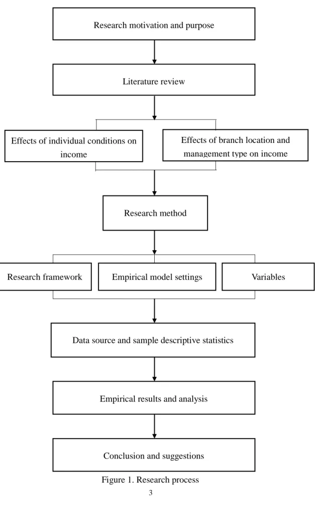
(10) store who have relationships that are both competitive and cooperative. The characteristics of branch stores or teams may thus affect the incomes of the real estate salespersons. Individuals belong to or are nested in branch stores and are affected by the overall system of the branch stores. The nested data structure can better be applied by using HLM (hierarchical linear modeling). Given the structure of a branch store system, how much variation in individual incomes is caused by individual factors and how much variation is caused by factors related to the branch stores or teams, and which characteristics of the branch stores affect the individual income differences between branch stores? These fundamental questions have not been answered by previous studies. The purposes of this research are as follows: 1) to use the null model, in which individual factors and branch store (or team) characteristic factors are not included in the model, to explore whether individual income variation causes significant differences between branch stores; 2) to use the intercepts-as-outcomes model to incorporate the individual-level independent variables in the first level to control the impact of these variables on individual income, and thereby explore the impact of the branch-store-level characteristic variables, such as management type and branch store location, on individual income; 3) to use the intercepts-and-slopes-as-outcomes model to explore whether the marginal impacts of the individual-level variables on individual income are moderated by management type.. 1.2 Research process The remainder of this paper is organized as follows: Section 2 is the literature review; Section 3 describes the research method, the reasons for using HLM, the variable settings, and the establishment of the empirical model; Section 4 presents the data 2.

(11) source and a description of the sample statistics; Section 5 discusses the empirical results analysis; and Section 6 offers conclusions and suggestions (see Figure 1).. Research motivation and purpose. Literature review. Effects of branch location and management type on income. Effects of individual conditions on income on the income. Research method. Research framework. Empirical model settings. Data source and sample descriptive statistics. Empirical results and analysis. Conclusion and suggestions Figure 1. Research process 3. Variables.

(12) 2. Literature review 2.1 The impacts of individual conditions on income Anderson, Byrd, and Hurst (2012) found that persons entering into real estate directly as a first career and those with experience in sales or retail perform significantly better than others with different backgrounds. Traditionally, human capital models are employed to analyze labor income or work performance. With regard to gender, Jud and Winkler (1999) used census data and other empirical data to show that women are significantly more likely than men to enter the real estate field. For men, the probability of entering the field grows with schooling up through four years of college, and declines thereafter. For women, the probability falls with increased schooling beyond high school. A career in real estate sales is more appealing to both men and women with more labor market experience. For women, however, as experience grows, the probability of choosing a real estate career rises less quickly, while for men, the probability grows with increasing experience . Seagraves and Gallimore (2013) suggested that although real estate was once a male-dominated field, females now account for approximately 60% of real estate agents in the United States. However, it is well established that women earn less than men in real estate sales. Glower and Hendershott (1988), Crellin et al. (1988), Sirmans and Swicegood (1997), and Jud and Winkler (1998) pointed out that the income of female salespeople is lower than that of men. More recently, Judge, Livingston, and Hurst (2012) suggested that men still earn more than women. These tendencies hold across cohorts and across occupations. In contrast, Abelson et al. (1990) argued that the income of female salespeople is higher than that of men. Follain et al. (1987) and Crellin et al. (1988) mentioned that working hours, schooling, working experience and agent license have significant impacts on the 4.

(13) income of a given real estate salesperson. When a real estate salesperson’s education level is higher, his or her income will also typically be higher (Follain et al. 1987; Glower and Hendershott 1988; Crellin et al. 1988; Abelson et al. 1990). Apparently, a real estate salesperson with a university degree typically has a higher income than does a high school diploma holder. However, the pay income of a master’s degree holder is not, on average, significantly higher than that of a high school diploma holder (Carroll and Clauretie 2000; Glower and Hendershott 1988; Jud and Winkler 1998). More recently, Lee and Shen (2008) also found that the working performances of housing agency employees may differ significantly because of different education levels. Specifically, the working performances of those with higher educational levels are better overall, and the working performances of housing agency employees with university degrees or more education are typically higher than those of housing agency employees with high school educations. In terms of age, Sirmans and Swicegood (1997; 2000) found that older age is correlated with lower income. Crellin et al. (1988) noted, however, that these results did not reach the 10% significance level. Abelson, Kacmar, and Jackofsky (1990) pointed out that actual age may therefore not be a determining factor of performance. Instead, it may be the age at whic h people begin a career in real estate that affects performance. The effect of age on earnings, meanwhile, was found to be insignificant by Crellin et al. (1988), Glower and Hendershott (1988) and Sirmans and Swicegood (1997). However, Follain et al. (1987) found that income increases with age until age 36 and then declines with age. Dulin (2004), in contrast, found that income increases 5.

(14) until age 50 and then decreases thereafter. With respect to marital status, Gray (1997) suggested that, on average, married men earn between 10 and 40 percent more than comparable men who have never been married. The empirical observation that married men earn higher wages than unmarried men is an empirical finding in labor economics. Ahituv and Lerman (2005) found that marriage increases men's earnings by about 20 percent and that marriage also results in a rise in wage rates and hours worked. A later study by Mercan (2011) showed that married men earn 27 percent more than single men and that married women earn 4 percent less than single women. Loughran (2002) and Gould and Paserman (2003) documented the negative effect of rising male income inequality on marriage rates, arguing that income dispersion extends the female search process. According to Mincer (1970), the expected performance of salespeople who are married and have children older than six years of age is higher than the expected performance of those who are married and have children under six. However, Abelson, Kacmar, and Jackofsky (1990) indicated that married people have a higher performance, but that the number of children has little effect on performance. Moreover, longer working hours on the part of real estate salespersons can result in higher incomes (Sirmans and Swicegood 1997; 2000; Abelson et al. 1990; Crellin et al. 1988; Glower and Hendershott, 1988; Follain et al. 1987). In addition, Abelson, 6.

(15) Kacmar, and Jackofsky (1990) pointed out that hours worked per week is also predicted to influence sales staff performance. Previous research examining this factor found that associates willing to work the longest hours achieve the most successful outcomes, and that the more hours worked per week, the better the performance. Generally speaking, general training (the accumulation of working experience) can result in higher incomes among real estate salespersons (Crellin et al. 1988; Frew and Jud 1986; Abelson et al. 1990; Jud and Winkler 1998; Glower and Hendershott 1988; Follain et al. 1987). According to empirical studies, working experience has a positive and significant impact on income and the working experience square has the negative impact. Lee and You (2007) suggested that working experience has a positive and significant impact on individual income; however, the effects of that influence will progressively decrease with the accumulation of work experience.. 2.2 The impact of branch location and management type on income The branch store characteristic is one of the important factors affecting an individual’s performance. According to Freeman and Kleiner (2005), fixed pay systems typically result in decreased output levels. Lazear (1986) pointed out that when the following conditions are found, adoption of a piece-rate pay system is more beneficial than use of a fixed pay system: (1) the cost to measure the output is very low; (2) the distribution of employee capabilities is relatively heterogeneous; (3) output measurement is unlikely to have errors; and (4) the cost to monitor product quality is very low. 7.

(16) According to Lazear’s analysis, a basic salary system is similar to a fixed pay system in that, under some conditions, the performance of an individual with a basic salary may be lower than that of an individual not receiving a basic salary. According to Yu and Liu (2004), a person receiving a basic salary is more likely to perform better than one who is not being paid at all . Heneman (1986) advocated performance-related pay, arguing that the members of an organization will increase their output in the case of performance-related pay. Lazear (2000) obtained the panel data of the employees of a major American vehicle glass manufacturing company to explore the adoption of a piece-rate pay system’s impact on employee productivity and company profit. The empirical findings suggested that employee productivity improved significantly by nearly 44%. Half of that impact could be attributed to the increased incentives while the other half of the impact could be attributed to the intention of highly productive laborers to choose to work in the company. As for the franchises and regular chains in Taiwan, regular chains use a pay system similar to the fixed basic salary system, and franchises use a pay system similar to the piece-rate pay system. Regarding the franchised and the non-franchised, Sirmans and Swicegood (1997) found that franchise affiliation increases income, and Carney and Gedajlovic (1991) found that a company would achieve the purpose of fast growth by franchising. Frew and Jud (1986) pointed out that the brand and reputation of the franchise system is very important to consumers who are not familiar with regional markets. As franchises can guarantee service quality, a franchising affiliation with a nationally known system can often increase the productivity of an agency, such as, for example, through the development of cases and sales. Therefore, they compared the performances of franchised and non-franchised stores, and found that franchised stores have more cases 8.

(17) and makes sales at higher prices. Crellin, Frew, and Jud (1988) used a sample of US real estate agency staff and showed that franchise system work has a negative impact on income. Benjamin, Jud, and Sirmans (2000), on the other hand, found that variables that did not have a significant effect on income include being affiliated with a franchise. Benjamin, Chinloy, Jud, and Winkler (2006) point out that a franchise offers a well-known brand name that signals information about the quality of the firm (including reliability) to new and existing clientele. These additional benefits can include marketing, training, and accounting services, and their findings indicated that franchisees have higher revenues, consistent with the potential benefits of a franchise. Such benefits can include enhanced name recognition, reductions in customer uncertainty, and assistance in marketing and training. However, net profits are not statistically significantly different between non-franchise firms and franchisees. This finding is consistent with the expectation that franchisors absorb the excess rents. Moreover, the net profit margin for franchisees is less than that of non-franchise firms. To compare the regular chains and franchises, Lee (1999) studied the impact of the management type on business performance. His theoretical model inferred that the franchises would be more active in the pursuit of profit maximization as the franchise system requires franchising fees. However, the empirical results suggested that there was no significant difference between the average sales volumes of regular chains and franchises, possibly because regular chains have more guarantees and higher quality requirements for employees, as well as better employee training. Therefore, a regular chain system typically results in a better reputation and increased competitiveness, improving operational performance. Hence, it can compete with a franchise system even if the latter 9.

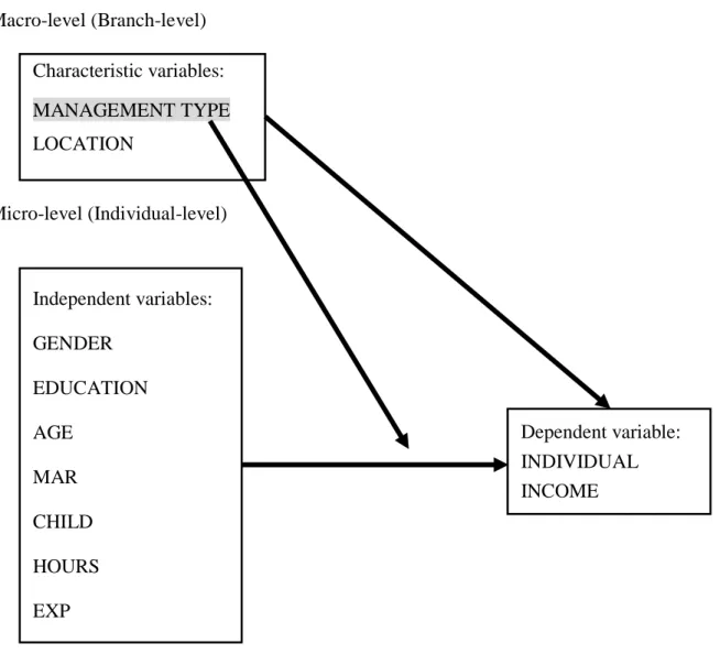
(18) provides high compensation incentives. Regarding variables related to the intermediary agency, branches closer to the downtown area usually have more business activity and higher transaction prices, resulting in better individual performance. Follain et al. (1987), Glower and Hendershott (1988), and Sirmans and Swicegood (1997) suggested that salespeople in the real estate industry who work in branches in downtown areas usually have higher incomes than those working in other areas. Sirmans and Swicegood (2000) found that licensee income is not affected by location. Average income for licensees in larger metropolitan areas is not significantly greater than t hat generated by their counterparts in less populated areas.. 3. Research method 3.1 Research framework The research framework for this study is shown in Figure 2. Individual-level independent variables (including GENDER, EDUCATION, AGE, MAR (marital status), CHILD (having a child aged six or younger), and HOURS) will affect individual income. Branch characteristic variables (including MANAGEMENT TYPE and LOCATION (branch location)) also affect individual income. And among the branch-level variables, the management type will moderate the impact magnitude of individual-level independent variables on individual income.. 10.

(19) Macro-level (Branch-level) Characteristic variables: MANAGEMENT TYPE LOCATION. Micro-level (Individual-level). Independent variables: GENDER EDUCATION Dependent variable: INDIVIDUAL INCOME. AGE MAR CHILD HOURS EXP. Figure 2 Research framework. 3.2 Empirical model settings This paper uses three HLM sub-models: the null model, the intercepts-as-outcomes model, and the intercepts-and-slopes-as-outcomes model. The dependent variable is individual income (Y), and is divided into high, medium, and low levels, where Y=1 represents agents with low incomes, Y=2 represents agents with medium incomes, and Y=3 represents agents with high incomes. The explanatory variables include GENDER, UNI (agents with an educational level of university or above), COLLEGE (agents with an educational level of college), AGE, CHILD (having a child aged under six or 11.

(20) younger), HOURM (per week working 41~70 hours), HOURH (per week working 71 hours and above), EXP (work experience), and EXPS (squares of work experience). The branch-level variables include TYPE (regular chains, franchises) and LOCATION (branch located in downtown or suburbs). Tabachnick and Fidell (2001) argue that centering can reduce the multicollinearity problems between explanatory variables. The types of centering can be classified into group mean centering and grand mean centering. In empirical estimation, the continuous variables will be applied for centralization by using grand mean.. 3.2.1 Null model This method tests whether individual incomes at various branches are different without considering any explanatory variables. The main purpose of the model is to distinguish intra-branch (intra-group) and inter-branch (inter-group) variation in individual income. It estimates how much variation in individual income is caused by the variation between branch stores and provides the preliminary estimated values for reference in the further analysis before considering whether HLM or general regression analysis should be applied. Utilizing terminology from Raudenbush and Bryk (2002), the model is characterized by level as follows:. Level-1 (micro-level):. mij  0 j  D2ij 2 j .........................................................................................................(1) where m is the ranking of income level, i is the agent, and. j is the. branch.  mij is the m th cumulative logit. As there are three levels in this paper, there are two cumulative logits. The term  2 j is the difference between the intercepts of the two logits. The term D2ij is a dummy variable 12.

(21) indicating whether m  2 (i.e., D2ij  1 if m  2 , D2ij  0 if m  1 ). This formulation thus summarizes the two equations:. 1ij   0 j  2ij   0 j   2 j ...........................................................................................................(2) Level-2 (branch-level):.  0 j   00  u0 j , u0 j ~ N (0,  00 )  2 j   2 .....................................................................................................................(3) where  0 j is the group mean of the high income agents in the j th branch,  00 is the overall average logit of high income agents, and u0 j is the random variation in the level-1 intercepts across branches, which represents the deviations of the j th branch’s mean logit from the grand mean or overall mean logit.. 3.2.2 Intercepts-as-outcomes model The intercepts-as-outcomes model mainly aims to validate the influence of explanatory variables at the micro-level and branch-level, if variables at both levels exist, on dependent variables. When the null model confirms that the inter-group variation in dependent variables is significant, the explanatory variables of agent characteristics are added at the micro-level, including GENDER, UNI, COLLEGE, AGE, MAR, CHILD, HOURM, HOURH, EXP, and EXPS. The intercept is set as a random effect. The model regards the influence of variables at the micro-level as constants. In other words, it assumes that branch-level characteristic variables are able to fully explain the variances of the dependent variables at the micro-level. Hence, TYPE j and. LOCATION j are specified to influence the intercepts of the micro-level prediction equations. By using the proposed model, this paper seeks to verify the impact of individual-level explanatory variables on individual income – that is, to determine 13.

(22) whether individual incomes are different under different management types and whether the individual incomes of agents working in downtown branches are better than those of agents working in outskirt branches. The model is characterized as follows:. Level-1 (micro-level):.  pmij     0 j  1 j GENDERij   2 jUNI ij   3 j COLLEGEij   4 j AGEij   1 p mij     5 j MAR   6 j CHILDij   7 j HOURM ij   8 j HOURHij   9 j EXPij  10 j EXPS ij.  mij  log.  D2ij 2 j ...................................................................................................................(4) Level-2 (branch-level):.  0 j   00   01TYPE j   02 LOCATION j  u 0 j , u 0 j ~ N (0,  00 )  kj   k0 , k  1 ~ 10.  2j   2 ...................................................................................................................(5) For three categories, a total of two cumulative logits are formulated. The term  mij is the m th cumulative logit; pmij is the probability of the m th income;  is the intercept or slope of the first level; and  is the intercept or slope of the second level. The term D2ij is a dummy variable indicating whether m  2 (i.e., D2ij  1 if m  2 ,. D2ij  0 if m  1 ).  2 j is the difference between the intercepts of two logits; u0 j is the error term, and is assumed to have a mean of zero and variance  00 ;  0 j is set as the random change; and  kj and  2 j are set as the constant change. The important feature of this model is that two intercepts are different, but the slope parameters are the same in each logit (Agresti, 1989). Because intercepts have a constant value for each of the two cumulative logits, this model is also called a proportional odds model. The terms  01 and  02 represent the cross-level direct impact of TYPE j and. 14.

(23) LOCATION j on the probability of high individual income.. 3.2.3 Intercepts-and-slopes-as-outcomes model The third model is the intercepts-and-slopes-as-outcomes model, which uses the intercepts and slopes of the individual-level as the outcome variables of the branch store level. It is a typical hierarchical linear model. The purpose of this model is to understand whether the characteristic variables of the branch stores can moderate the impact of the independent variables at the individual-level on the individual incomes. By using the management type (TYPE) as the moderating variable, this study explored whether the effect of the explanatory variables at the individual-level on the individual income (coefficient) can be moderated by the management type. Level-1 (micro-level):  pmij    mij  log    0 j  1 jGENDERij   2 jUNIij   3 jCOLLEGEij   4 j AGEij  1  pmij      5 j MAR   6 jCHILDij   7 j HOURM ij  8 j HOURHij   9 j EXPij  10 j EXPS ij  D2ij 2 j ..................................................................................................................(6). Level-2 (branch-level):.  0 j   00   01TYPE j   02 LOCATION j  u0 j , u0 j ~ N (0, 00 )  kj   k0   k 1TYPE j , k  1 ~ 10.  2j   2 ..........................................................................................................................(7). Finally, regardless of hierarchy, the single level ordinal logit model is applied for estimation. to. understand. the. differences. in. estimation. results. and. the. intercepts-and-slopes-as-outcomes model. The difference between the proposed model 15.

(24) and the intercepts-and-slopes-as-outcomes model is that, in the proposed model, the first level intercept  0 j is set as the fixed effect without the settings of random error item u 0 j . The model settings are as shown in Equation (8): Level-1 (micro-level):  pmij       GENDER   UNI   COLLEGE   AGE  log 1 p  0 j 1 j ij 2j ij 3j ij 4j ij mij     MAR   CHILD   HOURM   HOURH   EXP   EXPS  D  ........ (8) 5j 6j ij 7j ij 8j ij 9j ij 10 j ij 2ij 2 j. . mij. Level-2 (branch-level):.  0 j   00   01TYPE j   02 LOCATION j  kj   k0   k1TYPE j , k  1 ~ 10.  2j   2 ....................................................................................................................(9). 3.3 Variables The mode of operation for housing brokerage companies in Taiwan is the “branch”, and agents of the same branch are regarded as members of a “working team” who have a competitive-cooperative relationship. Hence, the variables can be divided into explanatory variables representing individuals and characteristic variables representing branches. The individual-level explanatory variables include dummy variables and continuous variables. The dummy variables for each agent include gender, educational level, marital status, whether the agent has children under six years old, management type, and branch location, while the continuous variables include age, work hours, 16.

(25) work experience, and square of work experience. The variables are defined as shown in Table 1. Individual income is measured by the value of the average annual income (including dividends and bonuses) of a respondent agent in the previous three years and is divided into high, medium, and low ranks, where Y =3 represents an agent with high annual income, Y =2 represents an agent with medium annual income, and Y =1 represents an agent with low annual income. It is notable that Rubin and Perloff (1993) and Booth and Frank (1999) used “income” as the proxy variable for performance or productivity. However, income reflects both performance and the employer's salary structure. Many studies (Glower and Hendershott, 1988; Crellin, Frew, and Jud, 1988; Sirmans and Swicegood, 1997; Jud and Winkler, 1998；Benjamin, Jud, and Sirmans, 2000) have pointed out that the income of female employees is lower than that of men. Carroll and Clauretie (2000) also confirmed that females earn less than males in real estate sales careers. In contrast, Abelson, Kacmar and Jackofsky (1990) argued that the income of female workers is higher than that of men. In this paper, if the agent is male, the variable is set to 1; otherwise, the variable is set to 0, and the expected coefficient is uncertain. Educational levels represent an investment in human capital. Richer accumulated professional knowledge can result in higher expected levels of performance. For 17.

(26) example, many authors (Follain, Lutes and Meier, 1987; Glower and Hendershott, 1988; Crellin, Frew, and Jud, 1988; Jud and Winkler, 1998; and Abelson, Kacmar, and Jackofsky, 1990) have found that schooling has a significant effect on income. Benjamin, Chinloy, Jud, and Winkler (2007) confirmed that a higher amount of schooling and experience creates efficiency and can reduce the number of hours worked. In other words, a higher level of schooling can result in higher expected income. In this paper, the educational levels of agents are divided into three categories: high school and vocational school; junior college; and university or above. The reference base is high school and vocational school, and two dummy variables are set. If the agent's educational level is college, the variable is set to 1; otherwise, it is 0. If the agent's educational level is university or above, the variable is set to 1; otherwise, it is 0. The coefficients of the two variables are expected to be positive in this paper. Thurow (1975) argued that the pay decrease caused by aging expected by the labor capital theory rarely takes place in actual fact, as previous experience had suggested. However, Sirmans and Swicegood (1997; 2000) did find that older workers have lower incomes. Crellin, Frew, and Jud (1988), meanwhile, noted that the association between older ages and lower incomes did not reach the 10% significance level. The empirical results of Crellin, Frew, and Jud (1988) showed that, as individuals grow older, it can be expected that their accumulated stocks of human capital may depreciate, and, 18.

(27) therefore, that their earnings may decline with age. A study released by the Department of Accounting and Statistics of Taiwan’s Executive Yuan (2008) titled “Study of Globalization’s Impact on Income Distribution” pointed out that the average pay of young workers was lower, while the income of the middle-aged increased with an expanding gap. In addition, the same department’s “Study on Statistics of Employee Characteristics and Differences” (Department of Accounting and Statistics, Executive Yuan, 2011) indicated that while age and pay were positively correlated, the impact on pay of age was only 1.49%. According to the empirical studies of Lee (2004), the income of older employees would be higher. Thus, the coefficient of the age variable in this study is expected to be a positive value. Mincer (1970) mentioned that married employees confirmed that they had higher performance. Korenman and Neumark (1991) also suggested that married men receive higher performance ratings than single men. Meanwhile, the aforementioned “Study on Statistics of Employee Characteristics and Differences” by the Department of Accounting and Statistics, Executive Yuan (2011), suggested that the pay of the married was slightly higher than the pay of the single. Under the same conditions, the pay gap was about 461 NTD. Therefore, in the case of family burden, the employee has relatively higher pressure to get a higher pay. According to Lee and You (2007), however, the performance of the married employees was relatively poorer. These 19.

(28) findings are consistent with the finding of Abelson, Kacmar, and Jackofsky (1990) that the performance of the married was lower as they had to devote more attention to familial obligations. Hence, their job performance would be affected. As such, we were uncertain as to what the impact of marital status on income would be in the present study. We expected that the coefficient of marital status can be positive or negative. Assaad and Zouari (2003) pointed out that the larger the number of children 6 and under a woman has, the less likely she is to participate in paid work. Parents have to spend more time taking care of children under the age of 6, and this can affect input into work. Mincer (1970) argued that employees with children under 6 generally had lower performance. As such, we expected that employees with children under 6 would have lower performance. Whether or not an agent had children aged 6 or younger was a variable in this study; if yes, its value was set to 1, but otherwise, it was set to 0. We expected that the coefficient would be negative. Longer daily hours worked usually indicates greater work effort and, thus, better performance (Follain, Lutes, and Meier, 1987; Glower and Hendershott, 1988; Crellin, Frew, and Jud, 1988; Sirmans and Swicegood, 1997; Abelson, Kacmar, and Jackofsky, 1990). We set the per week working hours as a dummy variable, with 40 hours as the reference basis. If HOURM is 41~70 hours, it is set to 1, otherwise, it is set to 0. If HOURH is 71 hours and above, it is set to 1, otherwise, it is set to 0. Hence, the 20.

(29) coefficient of the hours worked variable is expected to be positive. Many studies (Follain, Lutes, and Meier, 1987; Glower and Hendershott, 1988; Crellin, Frew, and Jud, 1988; Sirmans and Swicegood, 1997; Jud and Winkler, 1998) have shown that the longer that an individual has worked, the richer their working experience and the better their performance; thus, the coefficient of the years worked variable is expected to be positive. The square of years worked is used to represent the diminishing returns of work experience. It is thus expected that working experience has a positive and significant impact on individual income; however, the effects of that influence will progressively decrease with the accumulation of work experience. Lafontaine (1992), Shane (1996), and Shane and Foo (1999) found that franchising allows chains to perform better, presumably due to the better alignment of incentives. Sirmans and Swicegood (1997) used the labor capital model to analyze data from Florida, and found that franchises and agent income are positively correlated. Sirmans and Swicegood (2000) also analyzed data from Texas, however, and found that regional or national franchises’ agents did not have higher incomes than those of other agents. Crellin, Frew, and Jud (1988), meanwhile, found that earnings were substantially affected by franchise affiliation. On average, those associated with franchise firms earned 13.8% less. Perhaps franchise-affiliated firms employ less stringent personnel selection policies or provide less valuable on-the-job training. The 21.

(30) effect of franchise affiliation reported here conforms to the findings reported in a 1985 study of brokerage firm income and expenses conducted by the National Association of REALTORS. That study reported that franchise firms on average had lower profits and higher expenses than those not associated with a franchise. Beck et al. (2013) argued that franchise affiliation has historically offered a recognized brand and may have signaled greater quality service, especially to buyers who are new to an area or possess limited knowledge of local firms, but the advent of the digital age has diminished the competitive advantage of national affiliation. Nadal (2007) asserts that clients often conduct online research before contacting a brokerage firm. With MLS (multiple listing services) information becoming public, as opposed to being the exclusive domain of brokers and agents, residential real estate transaction information is available to anyone who has access to the internet. Beck et al. (2013) argued that the leveling of exposure across firms could explain the reduced value of a franchise affiliation in later years. Dajci, Boylan, and Cebula (2014) argued that, while earlier studies (Frew and Jud, 1986; Jud and Winkler, 1994) have found a non-negative association between franchise affiliation and firm earnings, a later study by Beck et al. (2013) found a negative association for the period 2006-2010 using data from Chatham County, Georgia. The branch store variables include the management types and locations of the branch stores. The management types included regular chains (e.g., Sinyi Realty, 22.

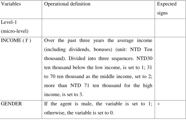
(31) Pacific Realtor regular chain, Yung Ching Realty regular chain) and franchises (e.g., Chinatrust Real Estate, Century 21 Real Estate LLC, Etwarm Real Estate, U-trust Real Estate, Yung Ching Realty, Taiwan Realty franchises, H&B Real Estate franchises). In this paper, Type is set to 1 for a regular chain and 0 for a franchise, and it is expected that the coefficient of management type is positive or negative. Intermediary agency branches closer to downtown areas have more business activity and higher transaction prices that result in better performance indicators. Sirmans and Swicegood (1997) suggested that agents in the housing brokerage industry who work in branches in the downtown area usually have higher incomes. Jud and Winkler (1999) have reported that earnings are positively associated with employment in a metropolitan area. Hence, in this paper, if a branch is located in the downtown area, the variable is set to 1; otherwise, it is 0. This paper expects that the coefficients of the branch store location are positive.. Table 1. Variable descriptions and definitions Variables. Operational definition. Expected signs. Level-1 (micro-level) INCOME ( Y ). Over the past three years the average income (including dividends, bonuses) (unit: NTD Ten thousand). Divided into three sequences. NTD30 ten thousand below the low income, is set to 1; 31 to 70 ten thousand as the middle income, set to 2; more than NTD 71 ten thousand for the high income, is set to 3.. GENDER. If the agent is male, the variable is set to 1; + otherwise, the variable is set to 0. 23.

(32) UNI. Educational level is divided into three categories. + High school and vocational school is the reference base, and dummy variables have been set. The variable is set to 1 for agents with an educational level of university or higher; otherwise, the variable is set to 0.. COLLEGE. If the agent has a college education, the variable is + set to 1; otherwise, the variable is set to 0.. AGE. The respondent’s age measured in years.. MAR. Marital status includes married and unmarried; it is +/--. +. a dummy variable. It is set to 1 if the agent is married; otherwise, it is set to 0. CHILD. It is set to 1 for having a child aged six or younger; -otherwise, it is set to 0.. HOURM,. The per week working hours of the respondents is +. HOURH. set as one of two dummy variables, with 40 hours as the benchmark: for HOURM, it is 1 for 41~70 hours, otherwise 0; for HOURH, it is 71 hours and above, otherwise, it is 0.. EXP. Work experience represented by number of years + working in the agent’s housing brokerage (unit: year).. EXPS. Square of work experience, as represented by the -square of the work experience variable.. Level-2 (branch-level) TYPE. Type make a dummy variable, regular chain store +/-set to 1, otherwise, the franchise is set to 0.. LOCATION. The branch located in Kaohsiung area, for example + Lingya District, Qianchen District set to 1, the other as Gushan District, Zuoying District, Fengshan District, Qianjing District is set to 0.. 24.

(33) 4. Data source and sample descriptive statistics 4.1 Data source This study conducted a questionnaire survey via mail of real estate salespersons in Kaohsiung from June 1, 2013, to July 31, 2013. The chain store (including regular chains and franchises) housing agency companies surveyed included Pacific Realtor (3 branch stores), Sinyi Realty (9 branch stores), Century 21 Real Estate LLC (3 branch stores), U-trust Real Estate (4 branch stores), H&B Real Estate (14 branch stores), Etwarm Real Estate (3 branch stores), Chinatrust Real Estate (7 branch stores), Taiwan Realty (7 branch stores) and Yung Ching Realty (16 branch stores), for a total of 66 branch stores. A total of 510 questionnaires were distributed, and 367 were retrieved. After eliminating 48 invalid samples, there were 319 effective samples from 54 branch stores, for an effective return rate of 62.55% (see questionnaire details in Appendix).. 4.2 Sample descriptive statistics The descriptive statistics for the individual-level are shown in Table 2. According to the distribution of the effective samples, in the previous three years, the percentage of the respondents with an average annual income of 310000-700000 NTD was 49.84%, the percentage of those with an average annual income of 710000 NTD or above was 28.21%, and the percentage of those with an average annual income of less than 300000 NTD was 21.95%. Regarding the proportion of male and female respondents, the male respondents accounted for 59.25% of all respondents, while the female respondents accounted for 40.75%. With regard to marital status, the unmarried accounted for 55.8%, while the married account for 44.2%. In terms of having a child or children aged 6 or below, respondents with a child below 6 accounted for 80.56%, while respondents without a child aged below 6 accounted for 19.44%. Regarding 25.

(34) education level, the respondents with a university degree accounted for 43.89%, followed by the respondents with a high school degree, who accounted for 27.90%. Regarding the average per week working hours, 41-70 hours was the range given by the most respondents, accounting for 70.53%, followed by 71 hours or above at 18.18%, and then 40 hours at 11.29%. The average age of the respondents was around 35.10, suggesting that most of the respondents are middle-aged. The average working experience of the respondents was around 5.73 years. The descriptive statistics of the branch store level are shown in Table 3. There were a total of 54 branch stores including 10 regular chain stores and 44 franchise stores. There were 13 branch stores located in the downtown area and 41 branch stores located in the suburbs.. 26.

(35) Table 2. Individual-level descriptive statistics (N=319) Variable Description. Effective. Classification. Times. percentage. Individual. less than 300000 NTD. 70. 21.95. income. 310000~700000 NTD. 159. 49.84. 90. 28.21. Male. 189. 59.25. Female. 130. 40.75. 710000 NTD - and above Gender Education. High school/. level. vocational school. 89. 27.9. College. 82. 25.71. 140. 43.89. Master. 7. 2.19. Doctor. 1. 0.31. 178. 55.80. 141. 44.20. 62. 19.44. 257. 80.56. University. Marital status Unmarried Married Having a. Having not. child aged 6. Having. and below Working. Less than 40 hours. 36. 11.29. hours. 41 hours~70 hours. 225. 70.53. 58. 18.18. 71 hours- and above Mean Age working experience. Standard deviation. Max.. Min.. 35.06. 9.04. 59. 21. 5.73. 6.22. 33. 1. As shown in Table 3, the 319 respondents were from 54 housing agency branch stores, including 10 branch stores of regular chains, accounting for 18.52% of the total. There were 13 branch stores located downtown, accounting for 24.07% of the total. 27.

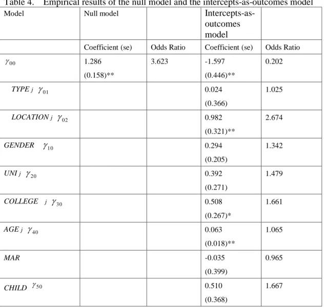
(36) Table 3 Branch- level descriptive statistics (N=54) Variable. Categories. Management type. Regular chain. 10. 18.52. Franchise. 44. 81.48. Downtown. 13. 24.07. Suburbs. 41. 75.93. Location of branch. Times. Percentage (% ). 5. Empirical results analysis. This study adopted HLM 6.1 version, SPSS19.0 software for estimations, including for the estimation of grand mean centered continuous variables. The analysis and explanations of the estimated results are as follows.. 5.1 Null model Table 4 provides the estimates for the null model. The estimate of  00 is 1.286 with a standard error of 0.158, reaching the 5% significance level. The random effects section shows the decomposition of the variance into its micro-level and branch-level components. The reported  2 statistic is 70.550 with 53 degrees of freedom. The results show that the variance at the branch-level is statistically significant, at better than the required 10% level of significance. This suggests that individual income vary across branches. When data are binary, within-group variability is defined by the sampling distribution of the data, typically the Bernoulli distribution. When the logistic model is applied, the level-1 residuals are assumed to follow the standard logistic 28.

(37) distribution, which has a mean of 0 and a variance of  2 / 3  3.29. This variance represents the within-group variance for ICC (intra-class correlation coefficient) calculations for dichotomous data, and the ICC can be similarly defined for ordinal outcomes (Snijders and Bosker, 1999). The null model for the intra-class correlation is: ICC . ˆ00. ˆ00  3.29. . 0.166  0.048 0.166  3.29. This suggests that 4.8% of the variation in individual income lies between branches.. 5.2 Intercepts-as-outcomes model The intercepts-as-outcomes model estimation results are shown in Table 4. For the impact of GENDER on income level, the estimated coefficient value is 0.294, which is not significant. The findings of many studies suggest that the working income of female workers is less than that of males (Glower and Hendershott, 1988; Crellin et al., 1988; Sirmans and Swicegood, 1997; Jud and Winkler, 1998 and Benjamin, Jud, and Sirmans, 2000). However, Abelson et al. (1990) argued that the working income of female workers is greater than that of males. This study concludes that the probability of a high income is higher among male workers than among female workers, but that the difference between the genders does not reach the level of significance.. The estimated coefficient value of educational level above university is 0.392, which does not reach the level of significance. The coefficient of estimation of 29.

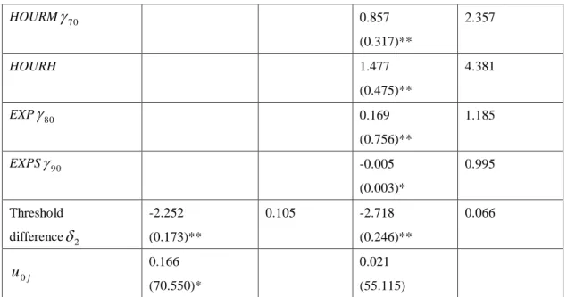
(38) educational level of college is 0.508, which does reach a 10% significance level. This suggests that the agents with an educational level of college do perform better in business than agents with high school or vocational school education. The estimation coefficient of AGE is 0.063 (Odds Ratio = 1.065), reaching the 5% significance level. This result is not consistent with the findings of Sirmans and Swicegood (1997; 2000), who found that older agents had lower incomes. This suggests that older agents have a higher probability of earning a high income. It further suggests that when serving housing agency clients, older agents may be able to increase their incomes due to their accumulated experiences in the realms of human resources and social interactions. The estimation coefficient of MAR is -0.035 (Odds Ratio = 0.965). According to Herman and Gyllstorm (1977), married workers have higher rates of FWC (family-to-work conflict) than the unmarried. The research findings suggest that marriage has a negative impact on the income without reaching the 10% significance level. Herr and Wolfram (2009) found that the birth of a child has a profound impact on the decision of women to exit the labor market, even among the highly educated. The estimation coefficient of “having children aged under six” is 0.510 (Odds Ratio=1.667). The empirical results are not consistent with the theoretical expectations, without reaching the 10% significance level.. In the respect of average weekly working hours, the estimation coefficient of average working hours (HOURM) is 0.857 (Odds Ratio=2.357), reaching the 5% significance level. The estimation coefficient of high average working hours (HOURH) is 1.477 (Odds Ratio=4.381), also reaching the 5% significance level. This suggests that the individual incomes of agents with median and high working hours are 30.

(39) significantly higher than those of agents with low average working hours. This finding is consistent with that of Follain, Lutes, and Meier (1987) and Glower and Hendershott (1988) that longer working hours result in better performance. A high number of agents with long working hours also implies that an agency has been in business for a long time. The coefficient estimate of EXP ,  80 , is 0.169 (Odds Ratio=1.185), which reaches the 5% significance level. The coefficient estimate of EXPS ,  90 , is -0.005, which reaches the 10% significance level. This suggests that increased work experience can help improve the income of agents; however, the effects of that influence will progressively decrease with the accumulation of work experience. This result is consistent with the conclusions of Glower and Hendershott (1988) and Sirmans and Swicegood (1997) to the effect that experience increases the performance of brokers or salespeople but, beyond a certain point, additional experience is of lesser value. According to the empirical results, the coefficients of GENDER, MAR, and CHILD do not reach the level of significance, indicating that these variables have no significant impact on individual income. As observed previously in the literature, a variety of influencing factors can, due to different sampling techniques, lead to inconsistent results among different studies. In particular, conflicting results often occur with regard to gender, race, franchise affiliation, and the agent’s age (Sirmans and Swicegood, 2000). Regarding the cross-level direct impact, the branch-level coefficient estimate of. TYPE j ,  01 , is 0.024, and does not reach a 10% significant level. According to empirical studies, the individual incomes of agents working for a regular chain are not significantly higher than those of agents working for franchises. This suggests that 31.

(40) there is no significant difference between the regular chain system and the franchise system in terms of their respective impacts on the probability of high agent income. In recent years, the developmental trends of the brokerage industry in Taiwan suggest that operational systems have considerably changed from the types based on the regular chain system, in which agents receive a high base salary, to types based on the franchise system, in which agents do not receive a base salary. This is evidenced by examples including Yongqing Housing, Pacific Housing, and Dong Sen Housing. Such changing trends can also be confirmed by empirical results. The individual incomes of agents working under the regular chain system are not significantly higher than those of agents working under the franchise system. The estimation coefficient of branch location is 0.982 (Odds Ratio = 2.674), which reaches a 5% significance level. This result suggests that the probability of better individual incomes among agents working in branches in the downtown area is higher than that among those working in branches in the suburbs, which confirms the findings of previous studies. For example, many studies (Follain et al., 1987); Glower and Hendershott, 1988; and Sirmans and Swicegood, 1997) have suggested that the incomes of agents working in the housing brokerage industry in metropolitan areas are higher than those of agents in outlying areas. Intermediary agency branches closer to downtown areas have more business activity and higher transaction prices, resulting in better income indicators.. In addition, according to the estimation results of the intercepts-as-outcomes model, the u0 j variance reached a significant level, indicating that the intercepts have random components and that other major branch-level characteristic variables have not been considered.. 32.

(41) 5.3 Intercepts-and-slopes-as-outcomes The intercepts-and-slopes-as-outcomes model estimation results are shown in Table 5. For the impact of GENDER on income level, the estimated coefficient value is 0.388, which is not significant. The findings of many previous studies suggest that the working incomes of female workers are lower than those of male workers (Glower and Hendershott, 1988; Crellin et al., 1988; Sirmans and Swicegood, 1997; Jud and Winkler, 1998; and Benjamin, Jud and Sirmans, 2000). However, Abelson et al. (1990) argued that the working incomes of female workers are greater than those of males. This study concludes that the probability of high income among male workers is higher than that among female workers, but that the difference does not reach the level of significance. The estimation coefficient of educational level above university is 0.303, which does not reach the level of significance. The coefficient of estimation of educational level of college is 0.427, which also does not reach a 10% significance level. This suggests that the agents with an educational level of college or an educational level above university do not perform better in business than agents with high school or vocational school educations. The estimation coefficient of AGE is 0.067 (Odds Ratio = 1.070), reaching the 5% significance level. This result is not consistent with the findings of Sirmans and Swicegood (1997; 2000), who found that older agents had lower incomes. This suggests that older agents have a higher probability of high incomes. The estimation coefficient of MAR is -0.041(Odds Ratio = 0.960), which also does not reach a 10% significance level. This result is not consistent with the findings of Abelson et al. (1990). They used the labor capital model to test the impact of marital status on performance, finding that married workers exhibit better performance. The estimation 33.

(42) coefficient of “having children aged under six” is 0.401 (Odds Ratio=1.493). Goldin (2006) argued that children were the most important factor related to out-of-work spells for women and a clear non-linearity exists in the impact of successive numbers of children. One child increased total time not at work by just 0.36 years on average, two children by 1.41 years, and three (or more) by 2.84 years. This result suggests that agents with children under the age of six have a greater probability of high income. The empirical results are not consistent with the theoretical expectations, without reaching the 10% significance level. Regarding the weekly average working hours, the estimation coefficient of the median average working hours (HOURM) is 0.969 (Odds Ratio=2.639), having reached the 5% significance level. The estimation coefficient of the high average working hours (HOURH) is 1.846 (Odds Ratio=4.81), having reached the 5% significance level. This suggests that the individual incomes of agents with median and high working hours are significantly higher than those of agents with low average working hours. This indicates that working in the housing agency industry imposes a time cost. In addition to the familiarity with specific laws and regulations, it requires more efforts in development, marketing sources of clients and case sources to get higher income. The results are consist with the findings of Glower and Hendershott (1988), Crellin, Frew, and Jud (1988), Abelson, Kacmar, and Jackofsky (1990), and Sirmans and Swicegood (1997) regarding working hours and income. The coefficient estimate of EXP,  80 , is 0.121 (Odds Ratio=1.129), which reaches the 10% significance level. The coefficient estimate of EXPS,  90 , is -0.004, which does not reach the 10% significance level. This suggests that increased work experience can help improve the income of agents; however, the effects of that influence will not progressively decrease with the accumulation of work experience. 34.

(43) This result is partly consistent with the conclusions of Glower and Hendershott (1988) and Sirmans and Swicegood (1997) to the effect that experience increases the performance of brokers or salespeople but, beyond a certain point, additional experience is of lesser value. According to the empirical results, the coefficients of GENDER, UNI, COLLEGE, MAR, CHILD, and EXPS do not reach the level of significance, indicating that these variables have no significant impact on individual income. As observed previously in the literature, a variety of influencing factors can, due to different sampling techniques, lead to inconsistent results among different studies. In particular, conflicting results often occur with regard to gender, race, franchise affiliation, and the agent’s age (Sirmans and Swicegood, 2000). Concerning the cross-level direct impact, the branch-level coefficient estimate of. TYPE j ,  01 , is 4.121, and does not reach the 10% significance level. According to empirical studies, the individual incomes of agents working for a regular chain are not significantly higher than those of agents working for franchises. This suggests that there is no significant difference between the regular chain system and the franchise system in terms of their respective impacts on the probability of high agent income. In recent years, the developmental trends of the brokerage industry in Taiwan suggest that operational systems have considerably changed from the types based on the regular chain system, in which agents receive a high base salary, to types based on the franchise system, in which agents do not receive a base salary. This is evidenced by examples including Yongqing Housing, Pacific Housing, and Dong Sen Housing. Such changing trends can also be confirmed by empirical results. The individual incomes of agents working under the regular chain system are not significantly higher than those of agents working under the franchise system. 35.

(44) The estimation coefficient of branch location is 1.100 (Odds Ratio = 3.003), which reaches the 5% significance level. This result suggests that the probability of better individual incomes among agents working in branches in the downtown area is higher than that among those working in branches in the suburbs, which confirms the findings of previous studies. For example, many authors (Follain et al., 1987); Glower and Hendershott, 1988; and Sirmans and Swicegood, 1997) have suggested that the incomes of agents working in the housing brokerage industry in metropolitan areas are higher than those of agents in outlying areas. Intermediary agency branches closer to downtown areas have more business activity and higher transaction prices, resulting in better income indicators. In addition, according to the estimation results of the intercepts-and-slopes-as-outcomes model, the u0 j variance did not reach a significant level, indicating that the intercepts do not have random components. Regarding moderating effects, the results indicated that management type can significantly moderate the marginal effect of UNI on individual income. This indicates that the incomes of those with a university and above degree are higher than the incomes of those with a high school or below degree. Moreover, this gap is higher in the case of the regular chain system than the franchise store system. In addition, the management type can significantly moderate the marginal effect of age on individual income. When the age is older, the expected individual income is higher, and the marginal effect of the regular chain system is lower than that of the franchise system. Management type can significantly and negatively moderate the marginal impact of working hours on individual income. This suggests that the individual incomes of those with median and high working hours are higher than those of agents with lower average working hours. However, the gap is smaller in the case of the regular chain system and the franchise system. The management type can also significantly and 36.

(45) positively moderate the marginal impact of working experience on individual income; that is, the positive impact of working experience on individual income is more significant in the case of the regular chain system than the franchise system. Moreover, the marginal effect of working experience on individual income will decrease with increasing working experience. The speed at which this decrease occurs is faster in the case of the regular chain system as compared to the franchise system. Finally, this study used the single level ordinal logit model to estimate the parameters. The estimation results suggest that the variable estimation coefficient and standard errors have no significant difference with intercepts-and-slopes-as-outcomes. This implies the robustness of the research estimation results. Table 4. Empirical results of the null model and the intercepts-as-outcomes model Model Null model Intercepts-asoutcomes model  00. Coefficient (se). Odds Ratio. Coefficient (se). Odds Ratio. 1.286. 3.623. -1.597. 0.202. (0.158)** TYPE j. (0.446)**.  01. 0.024. 1.025. (0.366) LOCATION j.  02. 0.982. 2.674. (0.321)** GENDER.  10. 0.294. 1.342. (0.205) UNI j.  20. 0.392. 1.479. (0.271) COLLEGE. j.  30. 0.508. 1.661. (0.267)* AGE j.  40. 0.063. 1.065. (0.018)** MAR. -0.035. 0.965. (0.399) CHILD.  50. 0.510 (0.368) 37. 1.667.

(46) HOURM  70. 0.857. 2.357. (0.317)** HOURH. 1.477. 4.381. (0.475)** EXP  80. 0.169. 1.185. (0.756)** EXPS  90. -0.005. 0.995. (0.003)* Threshold. -2.252. difference  2. (0.173)**. (0.246)**. 0.166. 0.021. (70.550)*. (55.115). u0 j. 0.105. -2.718. 0.066. * p<0.10, ** p<0.05. In the part of fixed effects, ( ) is the robust error; in the random effects part, ( ) is 2 the  value, the null model’s degree of freedom is 53, and the intercepts-as-outcomes model’s degree of freedom is 51.. Table 5. Empirical results of the intercepts-and-slopes-as- outcomes Model Intercepts and Ordinal logit slopes-asmodel outcomes.  00. Coefficient (se). Odds Ratio. Coefficient (se). Odds Ratio. -3.094. 0.045. -3.094. 0.045. (0.766)**. TYPE j.  01. 4.120. (0.766)** 62.500. (2.619) LOCATION j.  02. 1.100.  10. 0.388. 3.003. -0.870. 1.475. 0.303. 0.419. 1.965. 1.355. 0.427. 7.143. 1.540. -0.870. 0.419. 0.303. 1.355. 1.966. 7.143. (1.047)* 1.531. (0.321) TYPE j  31. 1.475. (0.305). (1.047)* COLLEGE  30. 0.388. (0.691). (0.305) TYPE j  21. 3.003. (0.259). (0.691) UNI  20. 1.100 (0.307)**. (0.259) TYPE j  11. 62.500. (2.619). (0.307)** GENDER. 4.121. 0.427. 1.531. (0.321) 4.673. (1.445). 1.540 (1.445). 38. 4.673.

(47) AGE  40. 0.067. 1.070. (0.018)** TYPE j  41. -0.159. TYPE j  51. -0.041. 0.853. 0.960. 0.401. 4.739. 0.687. 1.493. 0.969. 1.988. -2.927. 2.639. 1.846. 0.054. -3.363. 6.329. 0.121. 0.035. 0.543. 1.129. -0.004. 1.721. -0.015. 0.996. -2.813. difference  2. (0.204)**. u0 j. 2.639. -2.927. 0.054. 1.846. 6.329. -3.363. 0.035. 0.121. 1.129. 0.543. 1.721. -0.004. 0.996. (0.003) 0.985. (0.006)** Threshold. 0.969. (0.196)**. (0.003) TYPE j  101. 1.988. (0.073)*. (0.196)** EXPS  100. 0.687. (1.517)**. (0.073)* TYPE j  91. 1.493. (0.481)**. (1.517)** EXP  90. 0.401. (1.399)**. (0.481)** TYPE j  81. 4.739. (0.389)**. (1.399)** HOURH  80. 1.555. (1.288). (0.389)** TYPE j  71. 0.960. (0.388). (1.288) HOURM  70. -0.041. (1.267). (0.388) TYPE j  61. 0.853. (0.364). (1.267) CHILD  60. -0.159 (0.085)*. (0.364) 1.555. 1.070. (0.018)**. (0.085)* MAR  50. 0.067. -0.015. 0.985. (0.006)** 0.060. -2.813. 0.060. (0.204)**. 0.001 (52.980). * p<0.10, ** p<0.05. In the part of fixed effects, ( ) is the standard error; in the random effects part, ( ) is 2 the  value and the model’s degree of freedom is 51.. 39.

(48) 6. Conclusion and suggestions 6.1 Conclusion This study discussed the impact of individual-level characteristic variables including gender, education level, age, marital status, having a child aged below 6 or not, working hours, working experience, and branch-store-level characteristic variables such as management type and branch store location, on the individual incomes of real estate salespersons. According to the null model estimation results, individual incomes differ significantly among branch stores. Specifically, 4.8% of the variation in individual. income. is caused by differences. between. branch stores.. The. intercepts-as-outcomes model was applied in analysis, and showed that gender had a positive impact on individual income without reaching the significance level. Also, real estate salespersons with a college degree had significantly higher individual incomes than salespersons with a high school education. Age has a positive and significant impact on individual income, while marital status has a negative impact on individual income without reaching the level of significance. Having a child aged below 6 has a positive impact without reaching the significance level. Regarding the variable of average weekly working hours, the individual incomes of salespersons with long working hours are significantly higher than those of salespersons with short working hours. Working experience has a positive and significant impact on individual income, suggesting that age, working experience, and resources can help increase income. The working experience square coefficient is negative at the 5% significance level, suggesting that increased working experience can help increase income. However, accumulating work experience has a diminishing effect. In the respect of branch stores, the management type coefficient is positive without reaching the level of significance. The branch store location coefficient is positive at the 5% significance level, 40.

(49) suggesting that the incomes of real estate salespersons in branch stores located in the downtown area are higher due to more dense population, higher land and housing prices, and greater transaction opportunities. The intercepts-and-slopes-as-outcomes model was used to estimate the marginal value of using the branch store characteristic variables to moderate the individual-level independent variables. According to empirical studies, regarding the individual-level, gender has a positive impact on individual income without reaching the significance level. Two education level variables have a positive impact on individual income without reaching the significance level; age has a positive and significant impact on individual income; marital status has a negative impact on individual income without reaching the significance level; having a child aged below 6 has a positive impact on individual income without reaching significance level. The individual incomes of salespersons with long average weekly working hours are significantly higher, reaching the 5% significance level. Working experience has a positive and significant impact on individual income, and the impact of working experience square is negative without reaching the significance level. The coefficient of branch store management type is positive without reaching the significance level; the coefficient of branch store location is positive at the 5% significance level. Regarding the moderating effect, management type can moderate the impact of age on individual income. Old age can result in increased individual income, in particular, in the case of franchise stores. The management type can negatively moderate the marginal impact of working hours on individual income; in other words, longer working hours can result in increased individual income. However, the increase of the regular chain is less significant than the franchise stores. Management type can positively regulate the marginal effect of working experience on 41.