Mathematical Model of a Solar Module for Energy Yield Simulation in Photovoltaic Systems

Mathematical model of a solar module for energy yield simulation in photovoltaic systems

Weixiang Shen, Yi Ding, Fook Hoong Choo, Peng Wang, Poh Chiang Loh and Kuan Khoon Tan School of Electrical & Electronic Engineering

Nanyang Technological University 50 Nanyang Avenue, Singapore 639798

Abstract—This paper presents a new mathematical model of a solar module. Solar module temperature, solar radiation and its effect on series resistance are taken into account in the model.

The experimental data of the solar module under natural environment condition have been obtained to determine the model parameters. Then, the developed model is used to simulate energy yield of the solar module. This energy yield is compared with those obtained from experimental data and conventional approach. The results indicate that the proposed approach can have more accurate energy yield than conventional approach.

Thus, it can be useful for the design of PV systems.

Keywords-mathematical model; solar module; current-voltage characteristic; energy yield; simulation

I. I

Constantly increasing concerns of global warming and the depletion of oil have encouraged many countries in the world to adopt new energy policies to meet energy demand and preserve the environment. This leads to accelerating the research and development of renewable energy technology, especially solar energy in photovoltaic (PV) applications due to its free of pollution, silent operation, long life time and low maintenance [1-3]. In PV applications, solar module is a basic building block to construct PV systems through its connection in series or parallel. Therefore, the understanding of solar module characteristics is crucial for the design of PV systems.

A solar module typically consists of a number of solar cells in series. Each of these cells is basically a p-n junction capable of converting solar energy into electrical energy. The conventional technique to model solar cell is to establish mathematical expressions based on the equivalent circuits of the cell. Among these circuits, the circuit of a single diode model [4] as shown in Fig. 1 is widely adopted. In this circuit, I is the light-generated current which is a function of solar

radiation and cell temperature, I is the current to combine the

effects of the diffusion current from the base to emitter layers and the recombination current in the junction space charge region, I

is the current flowing through the shunt resistance R

representing the effect of leakage current flowing across the junction between the n and p layers, R

is the series resistance representing the losses due to current flowing through the highly resistive emitter and contacts, V and I are

Fig. 1 Equivalent circuit of a solar cell

terminal voltage and current of a solar cell, respectively. Based on this circuit, the cell current can be expressed in the one- diode model

ph d p

I ₌ I _{− − (1)} I I

where

[1 ( )]

ph phref c cref

ref

I I S T T

S α

= + − (2)

phref

I is the photocurrent at the standard testing conditions (STC), where the STC is referred to the conditions with the reference solar radiation S of 1000

W m at solar spectrum /

of AM 1.5 and solar cell reference temperature T

of 25°C.

S is an instantaneous solar radiation, α is the current temperature coefficient, T

is an instantaneous solar cell temperature, and

3

exp( / )(exp(( ) / 1))

d s c g c s t

I = k T − E nkT V IR + nV − ⁽³⁾

where k

is the photocurrent losses due to the charge carrier diffusion and n is a non-physically diode ideality factor, both of them can be obtained from parameter fits to the current- voltage (I-V) characteristics of the solar module. E

is the material bandgap energy (e.g. 1.12eV for silicon), V

is the thermal voltage depending on the cell temperature, Boltzmann’s constant ( k =1.38e-23) and the charge of the electron ( q =1.6e-19) and defined as

t c

/

V = kT q (4)

and

( ) /

p s p

I = V IR + R (5)

Usually the value of R

is very large and that of R

is very small, hence I

can be ignored [5-8], leading to the simplified one-diode model

ph d

I = I − I ⁽⁶⁾

Equations (1) and (6) are widely accepted as one-diode solar cell models in the design of the PV systems. To apply these solar cell models, two methods were developed to determine the model parameters. One method was to use curve-fitting to identify the parameters based on the experimental data of the solar cell or module under the specially controlled environment (SCE) with some special testing equipment, such as an expensive Sun simulator which can generate solar spectrum of

1.5

AM [9]. However, the SCE and Sun simulator are hardly available for most of PV system designers. The other method was to derive equations to calculate the model parameters directly based on the manufacturer’s datasheet of the solar module [4], [10] and [11], such as the open circuit voltage ( V

), the short circuit current ( I

), the voltage, current and power at maximum power point ( V

, I

and P

) under the STC. Since the STC does not represent what the PV systems are typically experienced in the field, namely natural environment condition (NEC), the model with the parameters obtained from the STC can hardly fit real I-V characteristics of solar cell or module under the NEC.

Different from conventional models, the neural network (NN) was explored to model solar module for mapping the input of solar radiation, ambient temperature and load voltage to the output of load current [12], [13]. This NN model is heavily dependent on the training data which may not cover the full range of the NEC. The neuro-fuzzy was also explored to model solar cell [14]. It required significantly fewer data than the NN model in [12], [13] by incorporating a priori knowledge derived from the physical model and datasheet of module [14].

But, the use of the solar cell temperature as the input of the neuro-fuzzy model made it difficult for real application because the direct measurement of solar cell temperature in the module is almost impossible. Some other models for solar cell or module, based on empirical approaches, were investigated to calculate the power and estimate energy production only [15], [16]. Since these models show no detailed description of I-V curves of solar module, they cannot be used to evaluate PV systems under the non-uniform conditions of solar module temperature and solar radiation [17].

This paper presents a new mathematical model for solar module. The solar module temperature on the backside, solar radiation falling on the solar module and its influence on the series resistance are taken into account in the model. The experimental data of the solar module obtained under the NEC are used to identify the model parameters. Then, the proposed model is used to simulate energy yield of solar module. The comparison of the energy yields among the proposed approach, experimental results and conventional approach has been

conducted. It shows that the proposed approach can have more accurate energy yield of the solar module than conventional approach, making it more suitable for PV system design.

II.

A. Experimental setup

One solar module of 200 W

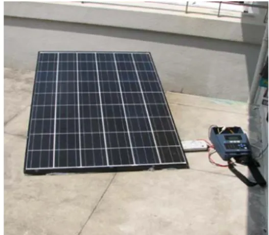
at the STC is adopted for testing. It situates on the building rooftop of School of Electrical and Electronic Engineering at Nanyang Technology University in Singapore. The module is mounted at the tilt angle of 15°, facing due south. The pyrometer situates besides the solar module at the same tilt angle, receiving the same solar radiation as the solar module. I-V checker is also installed besides the solar module. It can scan the I-V curves of the solar module together with solar radiation, solar module temperature and ambient temperature. Fig. 2 shows the experimental setup.

Fig. 2 Experimental setup for solar module under testing

The basic information of the solar module on the datasheet at the STC is shown as follows: the open circuit voltage ( V

)

=32.9V and its temperature coefficient ( α

)= -0.123 V/K, the

short circuit current ( I

) = 8.21A and its temperature

coefficient ( α

)= 0.00318A/K, the voltage at maximum power

point ( V

) =26.3V, the current at maximum power point

( I

) = 7.61A, and the power at maximum power point

( P

) = 200 W

. This solar module consists of 54 solar cells

connected in series with each of them 0.026 m

, adding up to a

total area of 1.41 m

. The experimentation of the solar module

is conducted under the NEC for modeling purpose. The

currents and voltages of the solar module together with the

solar radiations ranging from 344.83 to 977.36 W m /

and

solar module temperatures from 45.47 to 54.89 °C are collected

and stored in a data logger. Based on the observation and

analysis of the collected data, it is found that the I-V

characteristics of the solar module under the NEC are very

different from those on the datasheet under the STC due to the

significant difference between the NEC and the STC,

especially temperature. This motivates the development of a

new mathematical model for a solar module under the NEC.

B. Proposed model for solar module

The modeling of a solar module in this paper is only based on the experimental data of the solar module under the NEC, namely the I-V curves of the solar module and their corresponding solar radiations and solar module temperatures.

Once the model is developed, the I-V curves of the solar module can be predicted in the presence of the NEC and the energy yield of this module in the field can be reliably evaluated. The model should also be as simple as possible to reduce computational complexity. To this end, a new model of solar module is proposed by reasoning as follows.

• Solar module temperature ( T ). The solar cell temperature is widely used in the exiting solar cell models, but its direct measurement is almost impossible. The special experiment was conducted to determine the expression between solar cell temperature and solar module temperature [18].

However, this expression depends on the climatic conditions, surroundings and packing materials of a solar module, the expression obtained from one location may not be applied in another location.

Therefore, the solar module temperature (the backside temperature of the solar module) is adopted in the proposed model to establish the direct relationship between the I-V curves of the solar module and the solar module temperature.

• The photocurrent losses ( I

). A non-physically diode ideality factor ( n ) ranging between 1 and 2 is introduced in the photocurrent losses,

0 _m

( )

exp[(

) / (

)]

I = k T − E N nkT (7)

where n can be appropriately selected through the curve-fitting, N is the number of the solar cells in

series inside the module. To eliminate the coefficient k ,

I is computed by taking the ratio of (7) at two

different temperatures [5],

0 _ref( / _ref)3/ⁿexp{[( _g) / ( _s )](1/ 1/ _ref)}

I =I T T −E N nk T− T

(8)

where I

is the saturation current of a solar module at the reference condition.

• The series resistance ( R ). It is an important

parameter, especially for solar radiation and temperature far from the STC. Basically, two methods were developed to determine series resistance. One method was to calculate series resistance based on the equation directly derived from the known parameters on the datasheet given by manufacturers [10] and [11].

The other method was to measure series resistance by varying solar radiation and temperature under the SCE and then the relation of series resistance to solar radiation and temperature can be determined through the curve-fitting [9]. For commercial solar cells used in the module, series resistance is designed to be

approximately inversely proportional to the short circuit current at the STC [19], namely

1/ (40 )

s sc

R ≈ I (9)

According to (9), it reveals that series resistance is strongly dependent on short circuit current and thus solar radiation. Another research showed that series resistance is decreasing when the solar radiation is increasing [13]. Therefore, this paper proposes to extend (9) into the general form,

/ ( )

s s ph

R ⁼ N β I ⁽¹⁰⁾

where I can be any short circuit current under the

NEC including the short circuit current at the STC. β is a fitting parameter.

As a result, the proposed model for the solar module in which the number of the solar cells ( N ) are connected in

series is:

0

{exp[( ) / ( / )] 1}

m ph m m s s

I = I − I V + I R N nkT q − (11)

[1 ( )]

ph ref ref

ref

I I S T T

S α

= + − (12)

where I is the solar module current,

V is the solar module

voltage, α is the temperature coefficient of short circuit current. Equations (11) and (12) have a total of five parameters, namely I

, α , I , n ,

β . Once these five parameters are known, I-V curves of the solar module at the NEC can be easily generated, which can be used in the energy yield simulation of solar module in PV systems.

C. Parameter determination and model verification

As mentioned early, the experimental data of the solar module under the NEC are used to determine the parameters of (11) and (12). Since the data are obtained under the uncontrolled environment, two measures have been taken to preprocess the raw experimental data. Firstly, the developed program is used to filter out some irregular values in the I-V curves which have no physically accepted explanation, for example, the current value is increasing when the voltage value is rising. Secondly, the experimental data of short circuit currents to solar radiations and solar module temperatures for all the I-V curves are known to be linear. Thus, the linear least square method (LLSM) is used to analyze these data, if the presences of some of the data in the analysis lead to the negative temperature coefficient ( α ), the corresponding I-V curves are discarded. As a result, the preprocessed I-V curves corresponding to Table I are used in the modeling process.

According to the international standard IEC 60891, it

requires a minimum of five I-V curves to determine the

parameters in the solar cell model to translate I-V curves from

one combination of solar radiation and solar cell temperature

into another because the transformation in two dimensions is

usually required to determine four or five parameters in solar

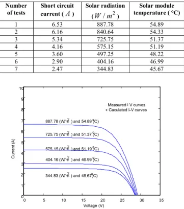
TABLE ISHORT CIRCUIT CURRENT, SOLAR RADIATION AND SOLAR MODULE TEMPERATURE

Number of tests

Short circuit current (

A

Solar radiation (

W m /

Solar module temperature ( °C) 1 6.53 887.78 54.89 2 6.16 840.64 54.33 3 5.34 725.75 51.37 4 4.16 575.15 51.19 5 3.60 497.25 48.22 6 2.90 404.16 46.99 7 2.47 344.83 45.67

Fig. 3 I-V curves under different combinations of solar radiation and solar module temperature

cell models [20]. Thus, the five I-V curves as shown in Fig. 3 corresponding to the number of the tests 1, 3, 4, 6 and 7 in Table I are chosen to model the solar module, where there are N I-V data pairs (

I

, V

) with j =1, 2, …, N

corresponding to five combinations of solar radiation and solar module temperature ( S ,

T ) with

i = 1, 2, …, 5. The remaining two I-V curves corresponding to the number of tests 2 and 5 in Table I are chosen to verify the model.

The two steps have been developed to reduce the complexity in determining the five parameters of I

, α , I ,

n and β . The first step uses the LLSM to identify two parameters of I

and α in (12). The relative percentage error (RPE) has been defined to show the accuracy of the calculated short circuit current ( I

) against the measured one ( I

),

( ) /

ph

cal mea mea

I

I

I

I

δ = − *100% (13)

where δ is the RPE. Table II shows the values of

I

and α identified by using the LLSM and their RPEs. The second step uses the non-linear least square method (NLSM) to identify the remaining three parameters of I , n and

β . The error function of the measured currents ( I

) at the given voltage, solar radiation and solar module temperature against

TABLE IIIDENTIFIED PARAMETERS (

I

α

δ

Measured short circuit current (

A

Calculated short circuit current (

A

RPEs (%)

I

α

6.53 6.54 0.16%

5.34 5.29 -0.90%

4.16 4.19 0.76%

2.90 2.91 0.31%

2.47 2.47 0.09%

the simulated currents is defined as

( ) ( )

ij mij mij

F x = I − f x (14)

where f

= I

− I

{exp[( V

+ I

R

) / ( N nkT q

/ )] 1} − , which is used to calculate the simulated currents, then the NLSM proceeds by finding a vector x = [ I , n ,

β ] that minimizes the sum of squares of the error function (14), namely

5 5

2 2

1 1 1 1

min ( ) min [ ( )]

i i

N N

ij mij mij

x x

i j i j

F x I f x

= = = =

= −

∑∑ ∑∑ ⁽¹⁵⁾

subject to the constraints: lb x ub ≤ ≤ , where lb = [0, 1, 10]

and ub = [1, 2, 100]. β is taken in the range of 10 to 100 through the observation of (9), where β is 40.

Two average errors have been defined to measure the accuracy of the developed model. One is the average percentage error for the current (APEC) to quantify each measured currents versus its corresponding simulated currents,

5 5

2

1 1 1

( ) /

Ni

cur mij mij i

i j i

I f N

δ

= = =

= ∑∑ − ∑ *100% (16)

The other is the average percentage error for the maximum power (APEMP) to quantify the measured maximum powers versus the corresponding simulated maximum powers,

5

, , ,

1

1 /

mpp

5

i

P P P

δ

=

= ∑ − *100% (17)

The reason to calculate the APEMP rather than average percentage error for the power at any points is that normally the PV systems are expected to operate in the maximum power points regardless of solar radiation and module temperature by including the maximum power point tracker. Table III shows the values of the parameters of I , n and

β identified by the NLSM, the APEC ( δ ) and the APEMP (

δ

).

With all five parameters, the calculated currents and

maximum powers from the developed model are compared

with the measured currents and maximum powers at the given

voltage, solar radiation and solar module temperature for the

experimental data used in the modeling process. The results for

TABLE IIIIDENTIFIED PARAMETERS OF

I

n

β

δ

APEMP(

δ

I

n β

δ

δ

0.000009 1.71 32.26 0.79% 2.87%

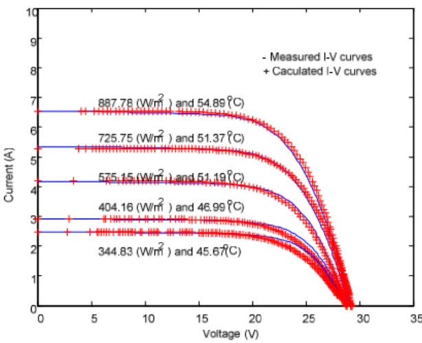
the comparison of the 5 I-V curves are shown in Fig. 4, with the APEC of 0.79% and the APEMP of 2.87%. It shows that the I-V curves from the developed model can match the I-V curves from the experimental data well, especially the I-V curves with higher solar radiation

Fig. 4 Comparison between the calculated currents and measured currents for the experimental data used in modeling process

Fig. 5 Comparison between the calculated currents and measured currents for the experimental data not used in modeling process

The comparison between the calculated currents and maximum powers from the developed model and the measured currents and maximum powers at the given voltage, solar radiation and solar module temperature for the experimental data not used in the modeling process is also conducted. The results for the comparison of 2 I-V curves are shown in Fig. 5, the corresponding APEC and APEMP are 0.51% and 2.94%, respectively. They agree with each other as well. It shows that the proposed model for the solar module under the NEC has a

reasonable accuracy in representing I-V curves and calculating power. Therefore, it can be used for energy yield simulation of solar module in PV systems.

III. E

Currently, power rating of solar modules is determined by their energy conversion efficiency under the STC and the total area of PV module. This rating leads to higher energy yield than that at the NEC due to high ambient temperature over a year in Singapore, which means if the PV systems are designed based on the energy yield at the STC they may not be able to deliver sufficient energy. To make the energy production of the designed PV systems more accurate, the developed model has been used for the energy yield simulation of solar module in PV systems.

The energy yield of solar module in one day from 10:00am to 2:40pm is simulated under Singapore weather conditions, which is then compared with those from both conventional approach and experimental results, where the proposed approach in this paper uses the developed model to find out the maximum power, the experimental approach applies I-V checker to obtain the maximum power and the conventional approach uses the maximum power at the STC and the temperature coefficients in the datasheet to calculate the maximum power at the NEC, all in the same period at the sampling rate of one minute. Thus, the energy yield ( E ) can

be estimated by

max, 1

1 60

M x

x i

i

E P

=

= ∑ ⁽¹⁸⁾

where E and

P

represent energy yield and maximum power evaluated either from the proposed model (m), or the experiment (e) or the conventional approach (c) expressed by

max,^c _i

( )

(25 ) 1

(

25)

P T = P ° C ^⎡ _⎣ + α T − ^⎤ _⎦ (19) and,

/ /

p V

V

I

α = α + α (20)

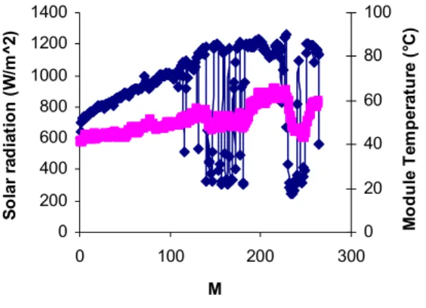
with x m e c = , , , respectively [21]. M is the number of the sampling points over the day. Figs. 6 and 7 show the experimental results of solar radiation, module temperature and maximum power during the period, respectively. Table IV shows the results of the energy yields of solar module for the above-mentioned three approaches. It can be seen that the RPE of the energy yield between the proposed model and experiment is 7.33% and the RPE of the energy yields between the conventional approach and experiment is 22.89%. It shows that the proposed model provide more accurate energy yield than the conventional approach, which can help to determine the size of the PV system in outdoor conditions more precisely.

TABLE IVENERGY YIELDS OF SOLAR MODULE AT DIFFERENT APPROACHES

E

(Wh) E

(Wh) E

(Wh)

622.97 580.40 713.24

0 200 400 600 800 1000 1200 1400

0 100 200 300

M

Solar radiation (W/m^2)

0 20 40 60 80 100

Module Temperature (°C)

Fig. 6 Solar radiation and module temperature

0 50 100 150 200

0 100 200 300

M

Maximum power (W)

Fig. 7 Maximum power of solar model

IV. C

The mathematical model is proposed to simulate energy yield of solar module in outdoor conditions. This model takes into account solar module temperature, solar radiation and its effect on series resistance. Both the LLSM and NLSM are used to identify the model parameters based on the experimental data of the solar module under outdoor conditions. The developed model is used to simulate the energy yield of solar module which is then compared with those obtained from the experimental results and the conventional approach. It indicates that the proposed approach can have more accurate energy yield of solar module than the conventional approach. Thus, the proposed approach enables the PV systems designers to determine the size of the PV systems more precisely in outdoor conditions. Furthermore, the proposed model can be extended to simulate energy yield of PV systems under non-uniform conditions of solar module temperature and solar radiation.

A

The authors would like to thank Aung Myint Khaing for his providing the experimental data of the solar module.

R

[1] G. Petrone, G. Spagnuolo, R. Teodorescu, M. Veerachary, M.

Vitelli, "Reliability Issues in Photovoltaic Power Processing Systems,"

IEEE Trans. on Industrial Electronics, vol. 55, no. 7, pp. 2569-2580, July 2008.

[2] Bialasiewicz, J.T., “Renewable Energy Systems with Photovoltaic Power Generators: Operation and Modeling,” IEEE Trans. on Industrial Electronics, vol. 55, no. 7, pp. 2752-2758, July 2008.

[3] C. Rodriguez, G.A.J. Amaratunga, "Long-Lifetime Power Inverter for Photovoltaic AC Modules," IEEE Trans. on Industrial Electronics, vol.

55, no. 7, pp. 2593-2601, July 2008.

[4] M.A. Green, Solar Cells, Englewood Cliffs, NJ: Prentice-Hall, 1982.

[5] G. Walker, “ Evaluating MPPT converter topologies using a Matlab PV model,” Journal of Electrical and Electronics Engineering, Australia, vol. 21, no. 1, pp. 49-55, 2001.

[6] Ali Naci Celik and Nasir Acikgoz, “Modeling and experimental verification of the operating current of mono-crystalline photovoltaic modules using four-and five parameters models,” Applied energy, vol.

84, pp. 1-15, 2007.

[7] Meza, C.; Negroni, J.J.; Biel, D.; Guinjoan, F., “Energy-Balance Modeling and Discrete Control for Single-Phase Grid-Connected PV Central Inverters,” IEEE Trans. on Industrial Electronics, vol. 55, no. 7, pp. 2734-2743, July 2008.

[8] Sera, D.; Teodorescu, R.; Hantschel, J.; Knoll, M., “Optimized Maximum Power Point Tracker for Fast-Changing Environmental Conditions,” IEEE Trans. on Industrial Electronics, vol. 55, no. 7, pp.

2629-2637, July 2008

[9] J.A. Gow, C.D. Manning, “Development of a photovoltaic array model for use in power electronics simulation studies,” IEE Proc.-Electr. Power Appl. Vol. 146, No. 2, pp. 193-200, March 1999.

[10] Sera, Dezso Teodorescu, Remus Rodriguez, Pedro , “PV panel model based on datasheet values,” IEEE International Symposium on Industrial Electronics, Vigo, Spain, pp. 2392-2396, 2007

[11] Ali Naci Celik, Nasir Acikgoz, “ Modeling and experimental verification of the operating current of mono-crystalline photovoltaic modules using four and five parameters,” Applied Energy, vol. 84, pp. 1-15, 2007 [12] L. Zhang and Yun Fei Bai, “ Genetic algorithm-trained radial basis

function neural networks for modeling photovoltaic panels,”

Engineering application of artificial intelligence, vol. 18, pp. 833-844, 2005.

[13] Engin Karatepe, Mutlu Boztepe, Metin Colak, “ Neural network based solar cell model,” Energy Conversion and Management, vol. 47, pp.

1159-1178, 2006.

[14] AbdulHadi, M.; Al-Ibrahim, A.M.; Virk, G.S., “ Neuro-fuzzy-based solar cell model,” IEEE Transactions on Energy Conversion, vol. 19, no.

3, pp. 619-624, Sept. 2004.

[15] K.H. Lam, J. Close, W. Durisch, “Modeling and degradation study on a copper indium diselenide model,” Solar energy, vol. 77, pp. 121-127, 2004.

[16] Wei Zhou, Hongxing Yang, Zhaohong Fang, “A novel model for photovoltaic array performance prediction,” Applied energy, vol. 84, pp.

1187-1198, 2007.

[17] Hiren Patel and Vivek Agarwal, “Matlab-based modeling to study the effects of partial shading on PV array characteristics,” IEEE Transactions on Energy Conversion, vol. 23, no. 1, pp. 302-310. March 2008.

[18] E. Skoplaki, J.A. Palyvos, “ Operating temperature of photovoltaic modules: A survey of pertinent correlation,” Renewable Energy, vol. 34, pp. 23-29, 2009.

[19] Wenham, S.R., Green, M.A., Watt., M.E., Corkish, R., Applied photovoltaics, Earchscan, 8-12 Camden High Street, London, NW1 0JH, HK, pp. 301-315, 2007.

[20] Procedures for temperature and irradiance corrections to measured I-V characteristics of crystalline silicon photovoltaic devices, IEC 60891, 2004.

[21] Eicker U., Solar technologies for buildings, New York: Wiley, ch. 5, 2003