國立台灣科技大學
資訊工程系
National Taiwan University of Science and Technology Department of Computer Science and Information Engineering
Four Families of Computation-Efficient Parallel Prefix Algorithms for Multicomputers
林彥君 Yen-Chun Lin 洪麗玲 Li-Ling Hung
Technical Report: NTUST-CSIE-08-01
February 2008
Abstract
Four families of computation-efficient parallel prefix algorithms for message-passing multicomputers are presented. The first two families generalize previous algorithms that use only half-duplex communications, and thus can improve the running time. The third and fourth families adopt collective communication operations to reduce the communication times of the first two, respectively. The precondition of all the presented algorithms is also derived. These families each provide the flexibility of choosing either less computation time or less communication time to achieve the minimal running time depending on the ratio of the time required by a communication step to the time required by a computation step.
Keywords: Computation-efficient; Cost optimality; Message-passing multicomputers; Parallel algorithms; Prefix computation
1. Introduction
The prefix computation is defined as follows: given n inputs x1, x2,…, xn , and an associative binary operator
⊕, compute yi = x1 ⊕ x2 ⊕…⊕ xi, for 1 ≤ i ≤ n. For ease of presentation, unless otherwise stated, this study assumes that xi’s and yi’s represent inputs and outputs, respectively, and the number of inputs is n. Prefix computation has been extensively studied for its wide application in fields such as biological sequence comparison, cryptography, design of silicon compilers, job scheduling, image processing, loop parallelization, polynomial evaluation, processor allocation, and sorting [1-3, 8, 11, 14, 16, 23-26, 28, 50, 52, 54, 55]. The binary operation ⊕ can be as simple as a Boolean operation or an extremely time-consuming multiplication of matrices [12].
Because of its importance and usefulness, prefix computation has been proposed as a primitive operation [4].
In fact, prefix computation is a built-in operation for Message-Passing Interface (MPI) parallel programming [17], and is implemented in hardware in the Thinking Machines CM-5 [49]. Additionally, numerous parallel prefix algorithms for various parallel computing models have been proposed [1, 7, 9, 13, 19, 24, 26, 29, 31, 35, 40, 41, 43, 45], and many parallel prefix circuits have also been designed [3, 5, 6, 10, 15, 18, 21, 25-27, 31-34, 36-39, 42, 44, 46, 47, 53-55].
Particularly, Egecioglu and Koc present a computation-efficient parallel prefix algorithm, henceforth named EK, for the half-duplex multicomputer model with p processing elements (PEs), where p < n [12]. Lin proposes an algorithm, henceforth named L, to reduce the communication time on the same model [30]. Half-duplex communication is the weakest communication model of message-passing multicomputers, with which each PE of a multicomputer can only send or receive a message in a communication step. This model of communication is basic and important [22]. Upper bounds of this model apply to other communication models, and lower bounds of this model are upper bounds for lower bounds of other models. Although a PE of a modern multicomputer can send and receive in the same step, it usually takes a longer time to send and receive than to send or receive only due to the inherent hardware capability and software overhead [20, 48]. On a p-PE system, the half-duplex communication ensures that no more than p/2 messages are transferred in a communication step and thus a communication step will not take too much time.
In this paper, four families of computation-efficient parallel prefix algorithms for message-passing multicomputers with p processing elements (PEs), where p < n, are presented. The first family of algorithms generalizes Algorithm L such that the family allows multiple combinations of the computation time and communication time. Algorithm L is just an extreme member of the family. The other members of the family take less computation time and may also take less communication time than Algorithm L does. We can thus take the exact time of performing ⊕ and that of communicating a message into account to use a member that requires the
minimal running time on a specific multicomputer. The communication time of the first family can be decreased to result in the second family, which is difficult to understand if the first family is not known.
For ease of programming and execution efficiency, collective communication operations, such as broadcast, can be better than a sequence of send or receive operations [51]. We thus use collective communications to further improve the communication time, and obtain one more family of algorithms from each of the first two families.
The rest of this paper is organized as follows. Section 2 presents the first family of parallel prefix algorithms for half-duplex message-passing multicomputers. Section 3 then derives the computation time and communication time, as well as other properties, of the first family. Section 4 shows how the communication time of the first family can be reduced to become the second family; the new communication time is also derived. Section 5 reduces the communication time by using collective communications; two more families of algorithms are thus obtained. Section 6 shows that the four families of algorithms are not always effective when p < n, and derives a much stronger precondition of the algorithms. Section 7 compares the algorithms for multicomputers. Conclusions are finally drawn in Section 8.
2. The first family of parallel prefix algorithms
In this section, we describe a family of parallel algorithms for solving the prefix problem of n inputs with p PEs, where p < n, on the half-duplex multicomputer model. A later section will elaborate the exact relation between p and n for the algorithms to be meaningful and useful. The p PEs are represented by P1, P2,…, Pp. For ease of presentation, i:j is used to represent the result of computing xi ⊕ xi+1 ⊕…⊕ xj, where i ≤ j. Like Algorithms EK and L, the proposed algorithms are more practical when the amount of time required to perform a binary operation ⊕ is greater than that required to transfer a message between two PEs. This situation may happen, for example, when the binary operation is time-consuming matrix multiplication.
Algorithm A(n, p, k) {Solving the prefix problem of n inputs, x1, x2,…, xn, using p PEs to generate y1, y2,…, yn, where n > p = kq + 1, k ≥ 1, q ≥ 1. In phase 1, k PEs are assigned to perform only computations; all the other PEs need to communicate among themselves, except when p – k = 1. To use this algorithm effectively, we show in a later section that n ≥ (p2 + kp + k + 1)/2 is required. For ease of presentation, assume that all numerical values are integers.}
Phase 1: Partition the inputs into two parts N1 = (x1, x2,…, xv) and N2 = (xv+1, xv+2,…, xn), where 0 < v < n. How the value of v is determined will be explained shortly. If p = k + 1, then P1 uses N1 to compute outputs y1, y2,…, yv sequentially; otherwise, P1, P2,…, Pp–k use N1 to compute y1, y2,…, yv by invoking A(v, p – k, k)
recursively. In the mean time, N2 is first distributed evenly among the other k PEs, Pp–k+1, Pp–k+2,…, Pp; each of the PEs holds c = (n – v)/k input values. These k PEs then take c – 1 parallel computation steps to compute
z1 = (z1,1, z1,2,…, z1,c), z2 = (z2,1, z2,2,…, z2,c),…, zk = (zk,1, zk,2,…, zk,c), respectively, where
zi,j = (v + (i – 1)c + 1):(v + (i – 1)c + j).
The value of v is chosen to make the total number of computation steps in this phase required by the first p – k PEs equal to that required by the other k PEs, and it is derived later. Note that yv is obtained by Pp–k.
Phase 2: Initially, Pp–k sends yv to all the other PEs. Next, Pp–k+1 scatters, i.e., partitions and distributes, z1 among all the PEs evenly, each PE having c/p of the c values. All the PEs then concurrently perform
yv+i = yv ⊕ z1,i, i = 1, 2,…, c, in c/p computation steps. Note that yv+c is computed by Pp.
Phase m (m = 3, 4,…, k + 1): Initially, Pp sends yv+(m–2)c to all the other PEs. Next, Pp–k+m–1 scatters zm–1 among all the PEs evenly, each PE having c/p values. All the PEs then concurrently perform
yv+(m–2)c+i = yv+(m–2)c ⊕ zm–1,i, i = 1, 2,…, c, in c/p computation steps. Note that yv+(m–1)c is computed by Pp.
Let C(n, p, k) denote the number of computation steps required by Algorithm A(n, p, k), and R(n, p, k) denote the number of communication steps. As in the two previous papers [12, 30], the initial input data loading time is not taken into account. To help understand the algorithm, we give two examples in the following. First, consider the case when p = 4, k = 3.
Phase 1: Assign N1 = (x1, x2,…, xv) to P1 and N2 = (xv+1, xv+2,…, xn) to P2, P3, P4. The prefixes of N1 are computed by P1, and N2 is processed by the other PEs. By the rule of deciding v, the number of computation steps required by P1, v – 1, equals the number of parallel computation steps required by the other three PEs, (n – v)/3 – 1.
Hence, v = n/4, and it takes n/4 – 1 computation steps in this phase. After phase 1 has completed, P1 obtains y1, y2,…, yn/4; P2 obtains z1,1, z1,2,…, z1,n/4; P3 obtains z2,1, z2,2,…, z2,n/4; and P4 obtains z3,1, z3,2,…, z3,n/4.
Phase 2: P1 initially sends yn/4 to P2, P3, P4 in 3 communication steps. Then, P2 sends 1/4 of the n/4 values obtained in phase 1 to each of the other three PEs in 3 communication steps. That is, z1,1 through z1,n/16, z1,n/8+1
through z1,3n/16, and z1,3n/16+1 through z1,n/4 are sent to P1, P3, P4, respectively. Subsequently, the four PEs compute n/4 outputs yn/4+1, yn/4+2,…, yn/2 in n/16 parallel computation steps. At the end, P4 has yn/2.
Phase 3: P4 initially sends yn/2 to the other PEs in 3 communication steps. Then, P3 sends 1/4 of the n/4 values obtained in phase 1 to each of the other three PEs in 3 communication steps. That is, z2,1 through z2,n/16, z2,n/16+1
through z2, n/8, and z2,3n/16+1 through z2,n/4 are sent to P1, P2, P4, respectively. Subsequently, the four PEs compute n/4 outputs yn/2+1, yn/2+2,…, y3n/4 concurrently in n/16 computation steps. At the end, P4 has y3n/4.
Phase 4: P4 sends y3n/4 and 1/4 of the n/4 values obtained in phase 1 to each of the other three PEs in 3 communication steps. That is, z3,1 through z3,n/16, z3,n/16+1 through z3,n/8, and z3,n/8+1 through z3,3n/16 are sent to P1, P2, P3, respectively. Subsequently, the four PEs concurrently compute n/4 outputs y3n/4+1, y3n/4+2,…, yn in n/16 computation steps.
Therefore, the total number of computation steps is
C(n, 4, 3) = (n/4 – 1) + n/16 + n/16 + n/16 = 7n/16 – 1. (1) The total number of communication steps is
R(n, 4, 3) = 3 × 2 + 3 × 2 + 3 = 15.
Next, consider the case when p = 7, k = 3.
Phase 1: Assign N1 = (x1, x2,…, xv) to the first four PEs, and assign N2 = (xv+1, xv+2,…, xn) to the last three PEs.
From Eq. (1), we know that P1, P2, P3, P4 can compute the prefixes of N1 in C(v, 4, 3) = 7v/16 – 1 computation steps. In the mean time, P5, P6, P7 share N2 evenly and compute their respective prefixes concurrently, taking (n – v)/3 – 1 computation steps. By the rule of deciding v,
7v/16 – 1 = (n – v)/3 – 1, v = 16n/37.
Consequently, each of the last 3 PEs has (n – v)/3 = 7n/37 input values. Thus, the values z1,1 through z1,7n/37 are obtained in P5, z2,1 through z2,7n/37 in P6, and z3,1 through z3,7n/37 in P7. Note that P4 obtains yv = y16n/37, and C(16n/37, 4, 3) = 7n/37 – 1.
Phase 2: P4 initially sends y16n/37 to the other six PEs in 6 communication steps. Then, P5 sends 1/7 of the 7n/37 values obtained in phase 1 to each of the other six PEs in 6 communication steps. Subsequently, the seven PEs compute 7n/37 outputs y16n/37+1, y16n/37+2,…, y23n/37 in n/37 parallel computation steps. At the end, P7 has y23n/37.
Phase 3: P7 initially sends y23n/37 to the other six PEs in 6 communication steps. Then, P6 sends 1/7 of the 7n/37 values obtained in phase 1 to each of the other six PEs in 6 communication steps. Subsequently, the seven PEs concurrently compute 7n/37 outputs y23n/37+1, y23n/37+2,…, y30n/37 in n/37 computation steps. At the end, P7 has y30n/37.
Phase 4: P7 initially sends y30n/37 and 1/7 of the 7n/37 values obtained in phase 1 to each of the other six PEs in 6 communication steps. The seven PEs then concurrently compute 7n/37 outputs y30n/37+1, y30n/37+2,…, yn in n/37 computation steps.
Therefore, the total number of computation steps is
C(n, 7, 3) = 7n/37 – 1 + (n/37) × 3 = 10n/37 – 1.
The total number of communication steps is
R(n, 7, 3) = R(16n/37, 4, 3) + 6 × 5 = 45.
In the next section, C(n, p, k), and R(n, p, k) in the general case, as well as other properties of Algorithm A, such as the values of p and k that lead to the smallest C(n, p, k) and R(n, p, k), are derived.
3. Properties of Algorithm A
Let v = αp,k n, where 0 < αp,k < 1. The value of αp,k is given in the following theorem.
Theorem 1. When p = k + 1, αp,k = 1/p; otherwise, αp,k = 2
2
1 1 p kp k p kp k
− + + + + + . Proof. Since the proof is very lengthy, it is given in the appendix.
Theorem 2. C(n, p, k) = 2 (2 ) 1 1.
n p k p kp k
+ −
+ + + Proof. We consider two cases separately.
Case 1: p = k + 1. In phase 1 of Algorithm A(n, p, k), P1 takes αp,k n – 1 computation steps to sequentially compute the prefixes of the αp,k n inputs assigned, and the number of computation steps required by the other k PEs is also αp,k n – 1. In phases 2 through k + 1, totally (n – αp,k n)/p computation steps are required to compute n – αp,k n values, precisely yv+1, yv+2,…, yn, by all the p PEs concurrently. Hence,
,
( , , ) p k, 1 n p kn.
C n p k n
p
α −α
= − +
From Theorem 1, , 1
p k p
α = ; thus,
2
/ 2 1
( , , ) n 1 n n p p 1.
C n p k n
p p p
− −
= − + = −
Since p = k + 1, we have
2
2
2
2 1
( , , ) 2 1
2
2 1
( 1)
2 ( )
1 1.
C n p k n p p n p k
p p k n p k p kp k
= − −
= + −
+ +
= + −
+ + +
Case 2: p = kq + 1, where q ≥ 2. The number of computation steps in phase 1 required by Pp–k+1 through Pp is
, 1.
n p kn k α
− −
As already mentioned in case 1, phases 2 through k + 1 require (n – αp,k n)/p computation steps. Hence, totally
, , ( )(1 , )
( , , ) (n p kn 1) n p kn n p k p k 1.
C n p k
p
k kp
α α α
− − + −
= − + = −
By Theorem 1, we then have
2 2
2
( )(1 1)
1 2 ( )
( , , ) 1 1.
1 p kp k
n p k
p kp k n p k
C n p k
kp p kp k
− + +
+ −
+ + + +
= − = −
+ + + Q.E.D.
We then investigate more on the effect of the values of p and k on the computation time. Let a = bq1 + 1, d = eq2 + 1, and b, e, q1, q2 ≥ 1. Then
2 2
2 2
2 2
2 ( ) 2 ( )
( , , ) ( , , )
1 1
( )( 1) ( 1)( )
2 .
( 1)( 1)
n a b n d e C n a b C n d e
a ab b d de e
a b d de e a ab b d e
n a ab b d de e
+ +
− = −
+ + + + + +
+ + + + − + + + +
= + + + + + +
Let num denote the numerator above, and it can be rewritten
num = ad2 + ade + ae + a + bd2 + bde + be + b − (a2d + abd + bd + d + a2e + abe + be + e)
= ad(d − a) + ad(e − b) + (ae − bd) + (a − d) + (bd2 − a2e) + be(d − a) + (b − e).
If a = d, then
num = a2(e − b) + a(e − b) + a2(b − e) + (b − e) = (e − b)(a − 1).
Clearly, if e > b, then num > 0, and thus C(n, a, b) > C(n, a, e); i.e., A(n, p, e) takes less computation time than A(n, p, b).
On the other hand, if b = e, then
num = ad(d − a) + b(a − d) + (a − d) + b(d2 − a2) + b2 (d − a)
= (d − a)(ad − b − 1 + ab + bd + b2).
Clearly, if d > a, then num > 0, and thus C(n, a, b) > C(n, d, b); i.e., A(n, d, k) takes less computation time than A(n, a, k).
Therefore, if d > a and e > b, then C(n, a, b) > C(n, d, b) > C(n, d, e). In other words, using as many PEs as possible and using the maximal k, which equals p – 1, can achieve the minimal computation time.
Theorem 3. R(n, p, 1) = p(p − 1);
R(n, p, k) = (2k − 1)(p – 1)(p + k – 1)/2k for k ≥ 2.
Proof. From Algorithm A, R(n, p, k) is the sum of the following four components:
(i) The number of communication steps, R(v, p – k, k), when the first p – k PEs perform A(v, p – k, k) in phase 1.
(ii) The number of communication steps required by Pp–k to send yv to the other p – 1 PEs in phase 2.
(iii) The number of communication steps required by Pp to send yv+ic to the other p – 1 PEs in phase i + 2, for i = 1, 2,…, k – 1.
(iv) The number of communication steps taken to distribute a total of kc, or n – v, values evenly among all the p PEs in phases 2 through k + 1. Note that the kc values are zi,j for i = 1, 2,…, k, and j = 1, 2,…, c, which are obtained in phase 1 of Algorithm A.
The value of R(n, p, k) depends on the values of p and k. Thus, we consider the following three cases.
Case 1: k = 1. The algorithm has only two phases, and it degenerates into Algorithm L. It has been shown [30]
R(n, p, 1) = p(p – 1).
Case 2: k ≥ 2 and p = k + 1. Component (i) is 0; component (ii) is p – 1; component (iii) is (k – 1)(p – 1), and component (iv) is k(p – 1). Note that in phase k + 1, component (iii) has the same communication source and destinations as component (iv). These two components can become one in phase k + 1; that is, p − 1 communication steps can be reduced. Hence,
R(n, p, k) = 0 + (p – 1) + (k – 1)(p – 1) + k(p – 1) − (p − 1)
= (p – 1)(2k – 1), (2) which is equal to (2k – 1)(p – 1)(p + k – 1)/2k since p = k + 1.
Case 3: k ≥ 2 and p = k(i + 1) + 1, where i ≥ 1. Component (i) is R(v, p – k, k). Components (ii), (iii), and (iv) are the same as those in case 2. Thus, using Eq. (2), we have
R(n, p, k) = R(αp,k n, p – k, k) + (p – 1)(2k – 1)
= R(αp–k,k αp,k n, p – 2k, k) + (p – k – 1)(2k – 1) + (p – 1)(2k – 1) .
. .
= R(αp–(i–1)k,k … αp–k,k αp,k n, p – ik, k) + (2k – 1)[(p – (i – 1)k – 1) + ... + (p – k – 1) + (p – 1)]
= R(αp–(i–1)k,k … αp–k,k αp,k n, p – ik, k) + (2k – 1)[i(p – 1) – (k + 2k + … + (i – 1)k)]
= R(α2k+1,k … αp–k,k αp,k n, k + 1, k) + (2k – 1)[i(p – 1) – ( 1) 2 ki i−
]
= R(α2k+1,k … αp–k,k αp,k n, k + 1, k) + 1 2 1
(2 1)[ ( 1) ( 1) ].
2
p k p k
k p p k
k k
− − − −
− − − − −
Since Eq. (2) can be rewritten
R(n, k + 1, k) = k (2k – 1), which is independent of the value of n, we obtain
R(n, p, k) = k (2k – 1) + (2k – 1)
2 2 1 2 2 1 3 3 2 2
( )
2
p p kp k p p kp k k
k k
− + − + − + − + +
−
= (2k – 1)
2 2 2 2
2 2 4 2 2 2 2 1 3 3 2
2
k p p kp k p p kp k k
k
+ − + − + − + − + − −
= (2k – 1)(p – 1)(p + k – 1)/2k. Q.E.D.
Theorem 3 reveals that the communication time is independent of n, provided that the precondition given in Section 6 is satisfied. It is easy to check that a smaller p results in less communication time. To see the effect of k, we first note that when k ≥ 2, a smaller k leads to less communication time. Next, we compare R(n, p, 1) and R(n, p, k), where k ≥ 2. From Theorem 3,
R(n , p, 1) – R(n, p, k) = (p2 – p) – (2k – 1)(p – 1)(p + k – 1)/2k
= (p – 1)(p – (2k2 – 3k + 1))/2k.
Therefore, when p ≥ 2k2 – 3k + 1, R(n, p, k) ≤ R(n, p, 1); otherwise, R(n, p, k) > R(n, p, 1).
Now, we can consider the running time, which is composed of the computation and communication times. As already mentioned, a larger k or p leads to less computation time. Consequently, when p ≥ 2k2 – 3k + 1 and k ≥ 2, A(n, p, k) is definitely faster than A(n, p, 1). However, it is not easy to decide the best values of p and k to achieve the least running time. Let τ be the ratio of the time required by a communication step to the time required by a computation step. Thus, the running time is equal to the time required to perform C(n, p, k) + τ R(n, p, k) computation steps, which can be minimized by choosing appropriate p and k values after taking τ into account.
From Theorem 2, C(n, p, k) = Θ(n/p); from Theorem 3, R(n, p, k) = Θ(p2). Totally, Algorithm A takes C(n, p, k) + τ R(n, p, k) = Θ(n/p) + Θ(p2) time. When n = Ω(p3), n/p = Ω(p2). Thus, Θ(n/p) + Θ(p2) = Θ(n/p). Since the sequential solution for the prefix problem takes Θ(n) time, Algorithm A is cost optimal when n = Ω(p3).
4. Reducing communication time
When p ≥ 2k + 1 and k ≥ 2, Algorithm A can be modified to become a faster algorithm named B. Recall that in the first phase of Algorithm A, the number of computation steps required by the first p – k PEs equals the number of computation steps required by the other k PEs. In addition, the first p – k PEs communicate among themselves in phase 1, but the last k PEs perform no communication operations; thus, the last k PEs are idle for the amount of time that the first p – k PEs take to communicate.
To reduce this idle time, we note that in Algorithm A there are communications among the last k PEs in phases 2 through k + 1, which can be performed in phase 1, but the communications involving the first p – k PEs in phases 2 through k + 1 should not be moved to phase 1. In each of these k phases, the original communications that can be moved to phase 1 are message transfers from any of the k PEs to the other k – 1 PEs. Thus, at most k(k − 1) communication steps can be moved to phase 1.
We need to make sure whether all or only part of the k(k – 1) communication steps should be moved.
Comparing k(k – 1) with the number of communication steps performed in phase 1 of Algorithm A, which is R(v, p – k, k), can clarify this. From Theorem 3,
R(v, p – k, k) = (2k − 1)(p − k − 1)(p − 1)/2k.
Since p ≥ 2k + 1, we have
R(v, p – k, k) ≥ (2k − 1)k(2k)/2k = k(2k − 1).
Thus,
R(v, p – k, k) – k(k – 1) ≥ k2 > 0.
That is, R(v, p – k, k) > k(k − 1). Therefore, the k(k – 1) communication steps can all be performed in phase 1 without increasing the communication time needed in phase 1. Clearly, Algorithm B(n, p, k) takes less communication time than Algorithm A(n, p, k). Note that the two algorithms take the same amount of computation time.
Let S(n, p, k) denote the number of communication steps required by Algorithm B(n, p, k). Thus, S(n, p, k) is the sum of the following components:
(i) S(v, p – k, k) communication steps required by the first p – k PEs invoking B(v, p – k, k) in phase 1.
(ii) p – 1 communication steps required by Pp–k to send yv to the other p – 1 PEs in phase 2.
(iii) (k – 1)(p – 1) communication steps required by Pp to send yv+ic to the other p – 1 PEs in phase i + 2, for i = 1, 2,…, k – 1.
(iv) k(p – k) communication steps taken to distribute part of zi, for 1 ≤ i ≤ k, evenly among P1, P2,… Pp–k in phases 2 through k + 1.
Note that in phase k + 1, since the communications that contribute to component (iii) and those that contribute to component (iv) are all sent out by Pp, the latter communications can be merged to the former ones, eliminating p − k communication steps in this phase. Let p = k(i + 1) + 1, where i ≥ 1. Hence,
S(n, p, k) = S(αp,k n, p – k, k) + (p – 1) + (k – 1)(p – 1) + k (p – k) – (p – k)
= S(αp,k n, p – k, k) + k(p – 1) + (k – 1)(p – k)
= S(αp–k,k αp,k n, p – 2k, k) + k(p – k – 1) + (k – 1)(p – 2k) + k(p – 1) + (k – 1)(p – k) .
. .
= S(αp–(i–2)k,k … αp–k,k αp,k n, p – (i – 1)k, k) + k[(p – (i – 2)k – 1) + ... + (p – k – 1) + (p – 1)]
+ (k – 1)[(p – (i – 1)k) + ... +(p – 2k) + (p – k)]
= S(αp–(i–2)k,k … αp–k,k αp,k n, p – (i – 1)k, k) + k[(i – 1)(p – 1) – (k + 2k + … + (i – 2)k)]
+ (k – 1)[(i – 1)p – (k + 2k + ...+ (i – 1)k)]
= S(αp–(i–2)k,k … αp–k,k αp,k n, p – (i – 1)k, k) + k ( 1)( 2)
[( 1)( 1) ]
2
i i k
i p − −
− − −
+ (k – 1) ( 1)
[( 1) ]
2 i i k
i p −
− −
= S(α3k+1,k … αp–k,k αp,k n, 2k + 1, k) + 2 1 2 1 3 1
[ ( 1) ]
2
p k p k p k
k p
k k
− − − − − −
− −
2 1 2 1 1
( 1)[ ]
2
p k p k p k
k p
k k
− − − − − −
+ − − .
As already mentioned, Algorithm B(n, p, k) takes k(k – 1) communication steps less than Algorithm A(n, p, k); that is, S(n, p, k) = R(n, p, k) – k(k – 1). From Theorem 3,
S(n, 2k + 1, k) = (2k – 1)(2k)(3k)/2k – k2 + k
= 5k2 – 2k.
Thus,
S(n, p, k) = 5k2 – 2k + 2 1 2 1 3 1
[ ( 1) ]
2
p k p k p k
k p
k k
− − − − − −
− − 2 1 2 1 1
( 1)[ ]
2
p k p k p k
k p
k k
− − − − − −
+ − −
=2 1 2 1 2
3 2.
2 2
k p p k k
k
− − + − +
Clearly, S(n, p, k) = Θ(p2). Therefore, the discussion of cost optimality of Algorithm A applies to Algorithm B.
That is, Algorithm B is also cost optimal when n = Ω(p3).
5. Using collective communications
In this section, we propose to reduce the communication time of Algorithms A and B when collective
communications are available. We first consider modifying Algorithm A to obtain a new one named E. In phase i + 2, where 0 ≤ i ≤ k – 1, of Algorithm A, the p – 1 transfers of yv+ic to all the other PEs can be replaced by a single broadcast to achieve the same effect. In addition, scattering of zi in phase i + 1, where 1 ≤ i ≤ k, can be done with a single scatter operation.
With a suitable implementation, either a broadcast or scatter operation takes Θ(log p) time to send to p PEs on a multicomputer [48]. Thus, broadcasting the k values yv, yv+c,…, yv+(k–1)c is equivalent to taking c1k log p point-to- point communication steps, where c1 is a constant, and k scatter operations are equivalent to taking c2k log p point- to-point communication steps, where c2 is a constant. Let c = c1 + c2 and p = k(i + 1) + 1, where i ≥ 0. We use T(n, p, k) to denote the number of communication steps required by Algorithm E(n, p, k), and consider the following three cases to examine T(n, p, k).
Case 1: k ≥ 2 and p = k + 1. The communications are k broadcast operations and k scatter operations. Thus, T(n, p, k) = ck log p = c(p – 1) log p = Θ(p log p).
Case 2: k ≥ 2 and p ≥ 2k + 1.
T(n, p, k) = T(αp,k n, p – k, k) + ck log p
= T(αp–k,k αp,k n, p – 2k, k) + ck log (p – k) + ck log p .
. .
= T(αp–(i–1)k,k … αp–k,k αp,k n, p – ik, k) + ck 1
0
log ( )
i j
p jk
−
=
∑ −
= T(α2k+1,k … αp–k,k αp,k n, k + 1, k) + ck
( 2 1) /
0
log ( )
p k k
j
p jk
− −
=
∑ − .
The first term of the right side of the above equation equals ck log (k + 1) since Case 1 gives T(n, k + 1, k) = ck log (k + 1). As for the second term, we have
ck
( 2 1) /
0
log ( )
p k k
j
p jk
− −
=
∑ − < ck
1
log
p i
= i
∑ = Θ(p log p).
Thus, T(n, p, k) = O(p log p).
Case 3: k = 1. Similar to the derivation of T(n, p, k) in Case 2, it has been obtained by Lin that T(n, p, 1) = Θ(p log p) [30].
Thus, we have T(n, p, k) = O(p log p). Moreover, since Theorem 2 gives C(n, p, k) = Θ(n/p), Algorithm E takes Θ(n/p) + O(p log p) time. If n = Ω(p2 log p), then n/p = Ω(p log p), and thus Θ(n/p) + O(p log p) = Θ(n/p).
Since the sequential solution for the prefix problem takes Θ(n) time, Algorithm E is cost optimal when n = Ω(p2 log p).
The modification to Algorithm B by using broadcast and scatter is very similar to the above modification, and
results in the same communication time complexity. Thus, the resulting algorithm, named F, is also cost optimal when n = Ω(p2 log p). Note that Algorithm F takes the same the number of computation steps as E.
6. Precondition of algorithms
In this section, we show that a relation stronger than p < n is required to use the proposed algorithms effectively. Indeed, a stronger relation among n, p, and k is needed. Before going into the general case, we first use two examples to shed some light.
Suppose n = 1024, p = 256, and k = 85. From Theorem 2, we have C(1024, 256, 85) < 7. However, it is even impossible to compute the sum of 1024 inputs in 7 computation steps. Therefore, Theorem 2 does not hold under this situation.
As a more general case, suppose n = 1024, p = 256 = kq + 1, and q ≥ 2. From Theorem 1, v = 1024(2562 – 256k + k + 1)/(2562 + 256k + k + 1) inputs are assigned to the first 256 – k PEs, and n – v = 2kpn/(p2 + kp + k + 1) = 512×1024k /(2562 + 256k + k + 1) < 8k inputs are assigned to the last k PEs. That is, each of the last k PEs has at most 8 inputs. Then, in phase 2, P257–k scatters at most 8 values to at most 8 of the 256 PEs for further computation, and thus at least 248 PEs are idle when the others are communicating and computing. This ineffective use of PEs also happens in phases 3 through k + 1.
Thus, in phase 1 at least kp inputs should be assigned to the last k PEs, which guarantees that in later phases each PE can be assigned at least one value to compute. Using n – v ≥ kp and Theorem 1, we see that
n – n(p2 – kp + k + 1)/(p2 + kp + k +1) ≥ kp, n ≥ (p2 + kp + k + 1)/2.
This is the precondition for running the presented algorithms effectively.
7. Comparison of algorithms
Lin and Lin present a parallel prefix algorithm named PLL for the half-duplex multicomputer [35]; PLL requires 2n/p + 1.44 log2 p – 1 computation steps and 1.44 log2 p + 1 communication steps when using p PEs, where 10 ≤ p < n. The number of computation steps of any of our algorithms is less than that of PLL, but the number of communication steps is greater than that of PLL.
Since Algorithm L is a special case of A(n, p, k), precisely A(n, p, 1), it takes C(n, p, 1) computation steps and R(n, p, 1) communication steps. We already know that a larger k results in less computation time. As for the communication time, we have shown that when p ≥ 2k2 – 3k + 1 and k ≥ 2, R(n, p, k) ≤ R(n, p, 1); otherwise, R(n, p, k) > R(n, p, 1). That is, A(n, p, k) is definitely faster than L when p ≥ 2k2 – 3k + 1 and k ≥ 2. However, when
p < 2k2 – 3k + 1, we need to know τ, the ratio of the time required by a communication step to the time required by a computation step, to decide which algorithm is faster.
Algorithm B can also be faster than Algorithm L. To compare their communication times, we see that when k
≥ 2,
R(n , p, 1) – S(n, p, k) = (p2 – p) – ((2k – 1)p2/2k – p/2 + k2 – 3k + 2)
= (p2 – kp – 2k3 + 6k2 –4k)/2k.
Therefore, when p2 – kp – 2k3 + 6k2 – 4k > 0, p ≥ 2k + 1, and k ≥ 2, Algorithm B is faster than Algorithm L;
otherwise, we need to know the value of τ to decide which is faster.
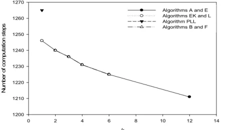
To help the reader understand the relative merits and drawbacks of algorithms, we give some example figures in the following. Fig. 1 shows the numbers of computation steps required when n = 8192 and p = 13. Note that k represents the number of PEs that perform no communications in phase 1 of our algorithms. Since PLL is a very different algorithm, it should not appear in the figures; however, for easy comparison, we show its related data in every figure as if k = 1. Clearly, Algorithms A and E each take the fewest number of computation steps when k = 12. Note that when 2 ≤ k ≤ (p – 1)/2, i.e., when Algorithms B and F are defined, the two algorithms each take the same number of computation steps as Algorithm A. Algorithm PLL takes the most, 1265, computation steps.
k
0 2 4 6 8 10 12 14
Number of computation steps
1200 1210 1220 1230 1240 1250 1260 1270
Algorithms A and E Algorithms EK and L Algorithm PLL Algorithms B and F
Fig. 1. The numbers of computation steps required when n = 8192 and p = 13.
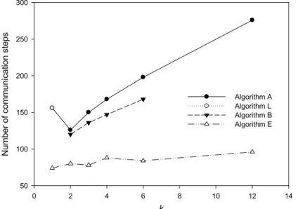
Fig. 2 shows the numbers of communication steps required by four algorithms. We assume that each collective communication involving p PEs requires the same amount of time as 2 log2 p point-to-point communications. Algorithm E takes the fewest communication steps among the four algorithms. As already mentioned, although the exact number of communication steps of Algorithm F is not derived, Algorithm F, when
defined, needs slightly less communication time than Algorithm E. Moreover, EK takes 3550 communication steps, which is too large to fit in the figure; PLL takes 7 communication steps, which is too small to fit in the figure.
k
0 2 4 6 8 10 12 14
Number of communication steps
50 100 150 200 250 300
Algorithm A Algorithm L Algorithm B Algorithm E
Fig. 2. The numbers of communication steps required when n = 8192 and p = 13.
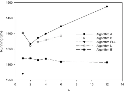
Note that τ has an impact on the total running time. If τ is small, which may be true when the binary operation ⊕ is matrix multiplication, our new algorithms are more probable to be faster than previous ones. For
example, Figs. 3 and 4 show the running times of algorithms when n = 8192 and p = 13, for τ = 1 and 0.1, respectively. When τ = 1, Fig. 3 shows Algorithm B is better than Algorithms A and L, but is worse than Algorithm E; Algorithm E is better than A, B, and L. In addition, Algorithm PLL is the fastest, which takes 1271 computation steps. In contrast, as shown in Fig. 4, when τ = 0.1, Algorithm B is generally faster than A and L, but Algorithm A(8192, 13, 12) is faster than Algorithm B(8192, 13, 6). Note that k = 12 is not valid for Algorithm B.
Algorithm E is faster than the others, and Algorithm E(8192, 13, 12) is the fastest. Note that since Algorithm F(8192, 13, 6) is only slightly faster than Algorithm E(8192, 13, 6), Algorithm E(8192, 13, 12) should be faster than Algorithm F(8192, 13, 6). In addition, Algorithm PLL is the slowest, which takes 1266 steps.
k
0 2 4 6 8 10 12 14
Running time
1250 1300 1350 1400 1450 1500
Algorithm A Algorithm B Algorithm PLL Algorithm L Algorithm E
Fig. 3. Running times in number of computation steps when n = 8192, p = 13, and τ = 1.
k
0 2 4 6 8 10 12 14
Running time
1210 1220 1230 1240 1250 1260 1270
Algorithm A Algorithm B Algorithm PLL Algorithm L Algorithm E
Fig. 4. Running times in number of computation steps when n = 8192, p = 13, and τ = 0.1.
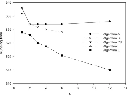
To contrast the running times when n = 4096 with those when n = 8192, Fig. 5 is given. Now Algorithm B(4096, 13, 6) is always faster than Algorithm A. Algorithm E is always faster than the others, and Algorithm E(4096, 13, 12) is the fastest. Moreover, Algorithm PLL takes 636 steps, which is worse than most of others.
k
0 2 4 6 8 10 12 14
Running time
610 615 620 625 630 635 640
Algorithm A Algorithm B Algorithm PLL Algorithm L Algorithm E
Fig. 5. Running times in number of computation steps when n = 4096, p = 13, and τ = 0.1.
With m-port communication, each PE has m input ports and m output ports to communicate with other PEs in one communication step, for some m ≥ 1. On a multicomputer of p (< n) PEs with m-port communication, a parallel algorithm, named M here, requiring 2n/p + (m + 1) logm+1 p – 2 computation steps and logm+1 p communication steps has also been presented [40]. The number of communication steps of Algorithm E or F is greater than that of Algorithm M. However, because Algorithm M needs more computation steps, Algorithms E and F may be faster than M when τ is small enough for their computation improvement to compensate for the communication disadvantage. Note that since M has a much stronger communication capability than the other algorithms, it is unfair to compare M with the others.
8. Conclusions
We have presented A(n, p, k), a family of parallel algorithms, run on half-duplex multicomputers with p PEs to solve the prefix problem of n inputs, where p = kq + 1, k ≥ 1, q ≥ 1, and n ≥ (p2 + kp + k + 1)/2. The numbers of computation steps and communication steps have been derived. When k is larger, a member algorithm takes less computation time and more communication time. This family is cost optimal when n = Ω(p3). Algorithm A is then modified to result in the second family, Algorithm B, which may run faster than A. Either A or B can be transformed into another family by adopting broadcast and scatter operations to reduce the communication time.
The resulting two families are cost optimal when n = Ω(p2 log p).
Each of the four families of algorithms provides the flexibility of choosing either less computation time (and more communication time) or less communication time (and more computation time) to achieve the minimal
running time. The key in choosing this and, more importantly, whether the running time is less than other prefix algorithms hinge on the ratio of the time required by a communication step to the time required by a computation step.
For all the presented algorithms, the last k PEs are idle for some amount of time in phase 1. Clearly, in phase 1, if we assign fewer than αp,k n inputs to the first p – k PEs and thus more than (1 – αp,k)n inputs to the last k PEs, then the first p – k PEs do fewer computations and the last k PEs do more. Therefore, the idle time can be eliminated, and the running time reduced. How many inputs should be assigned to the first p – k PEs is an open problem.
Appendix. Proof of Theorem 1 We consider two cases separately.
Case 1: p = k + 1. In phase 1 the number of computation steps required by P1 equals the number of parallel computation steps required by the other k PEs. That is,
,
, 1 p k 1.
p k
n n
n k
α −α
− = −
Thus,
,
1 1
1 .
p k k p
α = =
+ (3)
Case 2: p = kq + 1, where q ≥ 2. The number of computation steps in phase 1 required by P1 through Pp–k
equals that required by Pp–k+1 through Pp. That is,
,
( p k, , , ) n p kn 1.
C n p k k
k
α − = −α − (4)
Phases 2 through k + 1 require a total of (n – αp,k n)/p computation steps. Hence,
,
( , , ) ( p k, , , ) n p kn
C n p k C n p k k
p
α −α
= − +
, , ( )(1 , )
1 1.
p k p k p k
n n n n n p k
p
k kp
α α α
− − + −
= − + = − (5)
Substituting n and p in Eq. (5) with αp,k n and p − k, respectively, we obtain
,
, ,
(1 )
( , , ) 1.
( )
p k k
p k p k
C n p k k n p
k p k
α − =α −α−− − (6)
From Eqs. (4) and (6) we have
, ( , , , )
1 1,
( )
p k p k p k k p k
n n p n n
k k p k
α α α − α
− −
− = − −