國立宜蘭大學資訊工程研究所碩士論文

(1)

國立宜蘭大學資訊工程研究所碩士論文

Department of Computer Science and Information Engineering National Ilan University

Master Thesis

在 IEEE 802.16 WiMAX 的 Mesh 模式下的動態調整 Minislot 的分配機制

A Dynamic Minislot Allocation Scheme Based On IEEE 802.16 Mesh Mode

指導教授：趙涵捷博士

Han-Chieh Chao Ph. D.

研究生：林浩民撰

Hao-Ming Lin

中華民國九十七年七月

(2)

(3)

(4)

(5)

致謝

感謝趙涵捷教授不吝指導，以及提供完整的教育資源與實驗環境。在研究這個題目每每碰到瓶頸的同時，能夠為我指引方向，並且告訴我缺失與不足的地方，讓我能把研究做的更加的完善。也感謝陳懷恩教授，在英文撰寫方面的幫忙，

與論文疑點提醒。另外也感謝在背後支持我的學長、同學、朋友及家人，讓我能夠專心致力於研究議題上，並且與我一同討論是否有其他的可能性。

(6)

Abstract

IEEE 802.16 Standard leaves the minislot allocation in mesh mode for further

study. The minislot is the unit for resource allocation. The simple minislot allocation

scheme (SMAS) is proposed to allocate minislots according to the request from the

requester node. However, SMAS is not a flexible scheme, because it can not adjust the

request according to available minislots. We proposed a dynamic minislot allocation

scheme (DMAS) to improve the flexibility of SMAS with minimum change in

MSH-DSCH request Information Element (IE) field. The DMAS adds a Demand

Persistence field specified in MSDH-DSCH request IE and adjusts the field to reduce

the end-to-end delay and get better throughput compared to SMAS. This paper

introduces a new minislot allocation scheme (i.e. DMAS) and discusses the simulation

results.

Keywords：WiMAX、Mesh、802.16、Minislot

(7)

Figures

Figure 1-1-1: Example for the flow chart where node B’s request is rejected...3

Figure 1-2-1: Example 1 of node B’s request is rejected in the granter node’s resource map ...5

Figure 1-2-2: Example 1 of node B’s request is successful in the granter node’s resource map ...5

Figure 1-2-3: Example 2 of node B’s request is rejected in the granter node’s resource map ...6

Figure 1-2-4: Example 2 of node B’s request is successful in the granter node’s resource map ...6

Figure 2-2-1 Example: Flow chart of node B’s request was adjusted by granter node ...13

Figure 3-1 Average transmission time (in frames)...18

Figure 4-1 n × n Grid Topology ...21

Figure 4-2-1 Simulation result of Received Grant Count ...23

Figure 4-2-2 Simulation result of Granted Resources ...24

Figure 4-2-3 Simulation result of Throughput...25

Figure 4-2-4 Average End-to-End Delay ...26

(9)

Tables

Table 3-1 Evaluation parameters...17 Table 3-2 Average transmission time (in frames) ...19 Table 4-1 Simulation Parameter List ...20

(10)

Chapter 1 Introduction

1.1 Introduction of WiMAX Mesh Mode

The minislot is the unit for resource allocation in IEEE 802.16 that is also known as WiMAX. IEEE 802.16 Standard [1、2] leaves the minislot allocation in mesh mode for further study. The simple minislot allocation scheme (SMAS) [3、8] is proposed to allocate minislots according to node’s request. However, SMAS is not a flexible scheme, because it does not consider the status of the available minislots. We proposed a dynamic minislot allocation scheme (DMAS) to improve the flexibility of SMAS with a Demand Persistence field in MSH-DSCH Request Information Element (IE) field. The DMAS adjusts the Demand Persistence to reduce the end-to-end Delay, and get better throughput compared to SMAS.

In IEEE 802.16, Mesh mode has two kinds of scheduling mechanisms, one is centralized scheduling, the other is distributed scheduling. In the centralized scheduling, every packet is sent to the Mesh BS and then forwarded to the destination. Therefore, the Mesh BS can perform scheduling process and arrange the timeslot. The delay of connection setup is very long in centralized scheduling [3、20] because each node computes its retransmission time and last frame according to routing tree from the last MSH-CSCF (Mesh Centralized Schedule

(11)

Configuration) messages, newly received schedule, and some rules [20]. This paper focuses on the distributed scheduling.

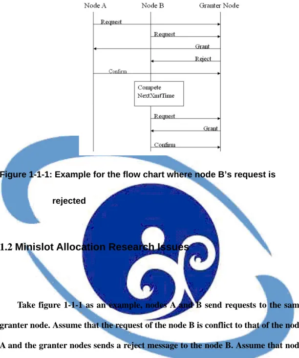
In the distributed scheduling, every node competes for channel access using a Mesh Election procedure based on the MSH-DSCH Scheduling IE of the two-hop neighbors. The minislots in data subframe are allocated based on a three-way handshaking mechanism by exchanging the request (MSH-DSCH Request IE), the grant (MSH-DSCH Grant IE, direction = 1), and the confirmation (MSH-DSCH Grant IE, direction = 0) among the nodes. Because the nodes only handle the messages within its two-hop neighbors instead of the entire mesh network, the distributed scheduling is more flexible and efficient on connection setup and data transmission. In distributed scheduling, every node computes its transmission time without global information. This may cause channel access control ineffective. When a requester node receives the grant message, it replies a confirm message to finish the three-way handshaking procedure with the granter node. If the requester node’s request is rejected by granter node, then the requester node should re-send the request. With the numbers of nodes increasing, then the three-way handshaking time will increase [3].

(12)

Figure 1-1-1: Example for the flow chart where node B’s request is rejected

1.2 Minislot Allocation Research Issues

Take figure 1-1-1 as an example, nodes A and B send requests to the same granter node. Assume that the request of the node B is conflict to that of the node A and the granter nodes sends a reject message to the node B. Assume that node A’s request contains the Demand Level = 256, and Demand Persistence = 128, node B’s request contains the Demand Level = 2 and Demand Persistence = 1 shown in figure 1-2-1, and the granter node get node A’s request first. Note that the Demand Level is number of minislots of the request, and the Demand Persistence is the number of persistence frames of the request.

The Demand Level and Demand Persistence are defined in MSH-DSCH

(13)

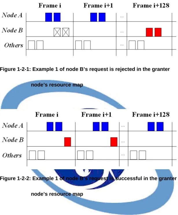
Request IE filed. After getting MSH-DSCH Request IE, the granter node calculates minislot range information according to the value of Demand Level divided by Demand Persistence. Minislot range represents how many minislots in a single frame. Because the limitation of Demand Persistence is 128 in IEEE 802.16 standard, node B will be rejected at first request. If the granter node can adjust the Demand Persistence of node B’s request to 2, then the granter node can grant minislot resource to node B as shown in figure 1-2-2.

Assume that node A has reserved one minislot in frame i at the pervious grant where node A’s request contains the Demand Level = 256 and Demand Persistence = 128. Node B’s request contains the Demand Level = 4 and Demand Persistence = 2 in figure 1-2-3. Assume that the granter node received node A’s request first. Node B will get reject message from the granter node because granter node cannot accept the Demand Persistence of node B’s request. If the granter node can adjust the Demand Persistence of node B’s request to 4, then the granter node can grant minislot resource to node B as show in figure 1-2-4.

The paper is organized as follows. We will describe the proposed dynamic minislot allocation scheme (DMAS) in section 2. In section 3, we use probability theory to analysis the single hop transmit time. Section 4 shows our simulation environment, and simulation results of DMAS were simulated by ns-2 simulator and compared with simple minislot allocation scheme (SMAS). The conclusion and future work are described in section 5.

(14)

Figure 1-2-1: Example 1 of node B’s request is rejected in the granter node’s resource map

Figure 1-2-2: Example 1 of node B’s request is successful in the granter node’s resource map

(15)

Figure 1-2-3: Example 2 of node B’s request is rejected in the granter node’s resource map

Figure 1-2-4: Example 2 of node B’s request is successful in the granter node’s resource map

(16)

Chapter 2 Dynamic Minislot Allocation Scheme

2.1 Simple Minislot Allocation Scheme

In Chapter 1, there have two examples in figure 1-2-1 and figure 1-2-3 to show that if granter node can adjust the request from node B, then node B won’t need to resend the request again. Based on this concept, we propose a dynamic minislot allocation scheme (DMAS) to solve this minislot allocation issue. Before we introduce DMAS, the simple minislot allocation scheme (SMAS) is described.

SMAS [3、8] is an allocation scheme used in IEEE 802.16 Mesh mode to allocate minislot. The basic concept of SMAS is finding the continuous minislots in persistence frames, and according to the IEEE 802.16 Mesh mode grant message, the start position and end position of continuous minislots in persistence frames need be the same as each persistence frame. The granter node rejected node B’s request in figure 1-2-1 and figure 1-2-3, because SMAS does not let granter node adjust the request based on the available minislot resource.

The node B needs to re-compete to reserve the minislot resource when the node B got reject message. Note that node B may not win the competition, and get resource so smoothly at frame i+128 in figure 1-2-1. In [3] proposed an analysis model to analysis the three-way handshaking procedure, and the average three-way handshaking delay is about 185 time slots in 100-node topology. The pseudo code of simple minislot allocation scheme is below.

(17)

# Pseudo Code of Simple Minislot Allocation Scheme

# While Granter node received a request from Requester node Got Request

# Calculate the numbers of minislot

Minislot Range = Demand_level / Demand Persistence Find the NextXmtTime of the requester

i=0

Counter = Demand Persistence;

While ( i < Counter ) do

If ( NextXmtTime + i*Ts ≦ minislots of S ≦ NextXmtTime + Range + i*Ts) are empty

Counter --;

Else

Return Fail # send reject to Requester End if

End while

Successful Grant, and send Grant message to Requester

# end of Simple Minislot Allocation Scheme

(18)

2.2 Dynamic Minislot Allocation Scheme

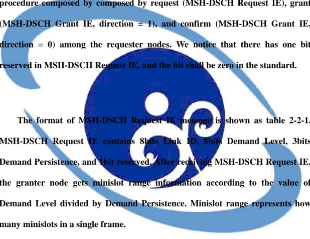
To reduce the delay of node B, we propose a dynamic minislot allocation scheme (DMAS). In IEEE 802.16 standard [1 、 2], three-way handshaking procedure composed by composed by request (MSH-DSCH Request IE), grant (MSH-DSCH Grant IE, direction = 1), and confirm (MSH-DSCH Grant IE, direction = 0) among the requester nodes. We notice that there has one bit reserved in MSH-DSCH Request IE, and the bit shall be zero in the standard.

The format of MSH-DSCH Request IE message is shown as table 2-2-1.

MSH-DSCH Request IE contains 8bits Link ID, 8bits Demand Level, 3bits Demand Persistence, and 1bit reserved. After receiving MSH-DSCH Request IE, the granter node gets minislot range information according to the value of Demand Level divided by Demand Persistence. Minislot range represents how many minislots in a single frame.

Table 2-2-1 MSH-DSCH Request IE Message format

Syntax Size Notes

MSH-DSCH_Request_IE(){

Link ID 8 bits

Demand Level 8 bits Demand Persistence 3 bits

Reserved 1 bit Shall be Zero }

(19)

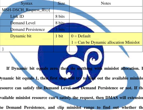
To enable DMAS, we use the reserved bit as the “Dynamic bit”, which is used to let granter node know that this request can be dynamic allocate when dynamic bit be set equal 1. The new MSH-DSCH Request IE message format is show as table 2-2-2.

Table 2-2-2 DMAS based MSH-DSCH Request IE Message format

Syntax Size Notes

MSH-DSCH_Request_IE(){

Link ID 8 bits

Demand Level 8 bits Demand Persistence 3 bits

Dynamic bit 1 bit 0 = Default

1 = Can be Dynamic allocation Minislot }

If Dynamic bit equals zero, then do notthing with minislot allocation. If Dynamic bit equals 1, then first step will try to find out the available minislot resource can satisfy the Demand Level and Demand Persistence or not. If the available minislot resource can’t satisfy the request, then DMAS will extension the Demand Persistence, and clip minislot range to find out whether the available minislot resource can satisfy the modified Demand Persistence and minislot range or not. DMAS will repeat these steps until granter node can find out an allocation way of modified Demand Persistence and minislot range or the Demand Persistence equals 128 (i.e., the limitation of IEEE 802.16 standard).

The pseudo code of dynamic minislot allocation scheme is below.

(20)

# DMAS Algorithm

Got Request

Successful Flag = 0;

While (Dynamic allocation bit = 1 && Demand Persistence <= 128) do

#Calculate the numbers of minislot

Minislot Range = Demand_level / Demand Persistence;

Find the NextXmtTime of the requester Counter = Demand Persistence;

i=0

While ( i < Counter ) do

If ( NextXmtTime + i*Ts ≦ minislots of S ≦ NextXmtTime + Range + i*Ts) are empty

Counter = Counter -1 Else

Extend Demand Persistence;

Return Successful Flag = 1;

End if

(21)

End while

If (Successful Flag =0)

Successful Grant, and send Grant message to Requester;

Else

Return Fail;

End if End while

# End of DMAS Algorithm

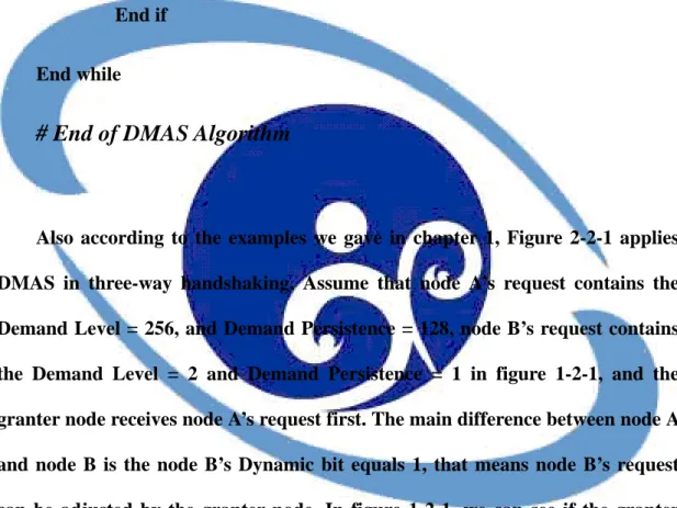
Also according to the examples we gave in chapter 1, Figure 2-2-1 applies DMAS in three-way handshaking. Assume that node A’s request contains the Demand Level = 256, and Demand Persistence = 128, node B’s request contains the Demand Level = 2 and Demand Persistence = 1 in figure 1-2-1, and the granter node receives node A’s request first. The main difference between node A and node B is the node B’s Dynamic bit equals 1, that means node B’s request can be adjusted by the granter node. In figure 1-2-1, we can see if the granter node cannot dynamically adjust node B’s request, node B will need to re-compete again. By applying DMAS, granter can dynamically adjust node B’s request from Demand Level equals 1 to Demand Level equals 2 according to the available minislot resource as show in figure 1-2-2. Then the granter node accepts the modified request of node B, and returns the Grant message which contains allocation information, the clipped minislot range, and the extended

(22)

Demand Persistence.

Figure 2-2-1 Example: Flow chart of node B’s request was adjusted by granter node

In figure 1-2-3, the node B’s request is rejected by the granter node because the granter node cannot accept the persistence of the node B’s request. By applying DMAS in figure 1-2-4, the granter node can dynamically extend the persistence of node B’s request, and clip the minislot range in a frame to fit the Demand Level of node B’s request.

(23)

Chapter 3 Performance Analysis

Dynamic allocation scheme is proposed to enhance the flexibility of minislot allocation, and reduce the delay of minislot allocation. We try to use probability theory to analysis transmission time between requester node and granter node.

The transmission time is the interval between the request had been send by requester node and granter node received the compete packet. Assume SMAS_T_{avg_Tran} is the average transmission time of a requester node based on SMAS. Psu is the successful rate of request has been accepted by granter node on SMAS. We can express the average transmission time as (1).

( ) ( ) ( )

∑ ⁻ ^⋅ ⁺ ^⋅ ⁺ ⁺

=

ⁿ _su ⁿ _allocate _su _allocate _PHY _frame

Tran

Avg

P n T P T T T

T SMAS

1

_

1 _

(1)

In (1), T_PHY is propagation time, and T_frame is transmit time of persistence frames. Tframe can be calculated from frame duration in WiMAX standard and Demand Persistence in MSH-DSCH Request IE filed. Tallocate is the sum of competition time T_compete with other nodes and three-way handshaking time T_thr as (2).

(24)

thr Compete

allocate

T T

T = +

(2)

The successful rate Psu is decided by number of nodes wants to reserve the minislot resources, minislot range, and frame persistence of each request. Then we can express the Psu as (3). M is the number of minislots in a single data subframe, and m is the minislot range of the request. Ncompete is the number of requester node’s two-hops neighbor nodes. We can predict the successful rate in a single frame by using these three parameters. Per is the number of persistence frames of request.

( )

^Per

N N

su _compete

compete

M m

P M ⎟⎟

⎠

⎜⎜ ⎞

⎝

⎛ −

=

(3)

We also can use probability theory to analysis the average transmission time of requester node based on DMAS. The average transmission time shows as (4).

In (4), DMAS_Tavg_Tran is the average transmission time of a requester node based on DMAS. Assume PD_su is the successful rate of request has been accepted by granter node on DMAS. T’_frame is transmit time of persistence frames according

(25)

to the extended Demand Persistence. We can see the different between SMAS_Tavg_Tran and DMAS_Tavg_Tran is the successful rate and transmission time of persistence frames.

( ) ⁽ ⁾ ( )

∑

⁻ ^⋅ ⁺ ^⋅ ⁺ ⁺

= ⁿ _D _su ⁿ _allocate _D _su _allocate _PHY _frame

Tran

Avg P n T P T T T

T DMAS

1

_ _

_ 1 '

_

(4)

Because DMAS may extend the Demand Persistence in MSH-DSCH Request IE field, we need consider the successful rate of original Demand Persistence, and extended Demand Persistence. (4) shows the successful rate based on DMAS. We can see the first term is equal to Psu, and the other terms mean the successful rate of Demand Persistence had been extend to 2x, 4x, 8x, 32x, and 128x. One goal of DMAS is improve the flexibility with minimum change in IEEE 802.16 standard. The extension multiple need fixed with IEEE 802.16 standard, so DMAS will extend 2x, 4x, 8x, 32x, and 128x according to the Demand Persistence.

To evaluate the average transmission time, we apply some parameters from [1、2、3]. The parameters are show in table 3-1. In [3], T_compete needs 185 control slots and Tthr needs 19 control slots when the network has 100 nodes. We choose

(26)

IEEE 802.16 standard. Also we choose the maximum value of the opportunities in single control subframe in IEEE 802.16 standard.

( )

128 32

8 4

2

_

128 32

8 4

2

×

⎟ ⎟

⎟

⎠

⎞

⎜ ⎜

⎜

⎝

⎛

⎟⎟ ⎠

⎜⎜ ⎞

⎝

⎛ ⎥⎦ ⎤

⎢⎣ ⎡−

− +

⎟ ⎟

⎟

⎠

⎞

⎜ ⎜

⎜

⎝

⎛

⎟⎟ ⎠

⎜⎜ ⎞

⎝

⎛ ⎥⎦ ⎤

⎢⎣ ⎡−

−

+

⎟ ⎟

⎟

⎠

⎞

⎜ ⎜

⎜

⎝

⎛

⎟⎟ ⎠

⎜⎜ ⎞

⎝

⎛ ⎥⎦ ⎤

⎢⎣ ⎡−

− +

⎟ ⎟

⎟

⎠

⎞

⎜ ⎜

⎜

⎝

⎛

⎟⎟ ⎠

⎜⎜ ⎞

⎝

⎛ ⎥⎦ ⎤

⎢⎣ ⎡−

−

+

⎟ ⎟

⎟

⎠

⎞

⎜ ⎜

⎜

⎝

⎛

⎟⎟ ⎠

⎜⎜ ⎞

⎝

⎛ ⎥⎦ ⎤

⎢⎣ ⎡−

−

⎟⎟ +

⎠

⎞

⎜⎜ ⎝

⎛ −

=

Per

N Per N

N

Per

N Per N

N

Per

N

N Per

N N su

D

compete

compete compete

M M m

M m P M

(5)

Table 3-1 Evaluation parameters

Topology Grid T_compete (avg. time of wins the competition) 19 control slots

Tthr (three-way handshaking time) 185 control slots M (numbers of minislots in single frame) 256 minislots

Opportunities in single control subframe 16

Demand Level 128

Demand Persistence 4

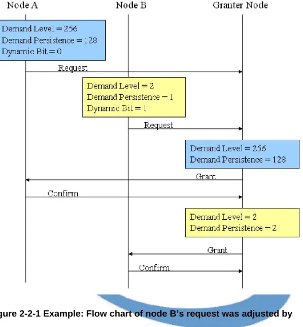
Figure 3-1 shows the evaluation result of average transmission time. We can

(27)

see the number of been rejected times increase, the average transmission time increase. We also can see that SMAS need more frames to complete the transmission than DMAS. Table 3-2 shows DMAS is better than SMAS if requester node got reject more than once. Based on the evaluation result, if the network has ocean traffic and lots of compete nodes, SMAS will need more frames to complete transmission than DMAS. In the evaluation, we only analysis single-hop transmission time, then we can expect that DMAS will get lower the end-to-end delay than SMAS. The simulation results will prove our evaluation analysis in session 4.

Average Transmission Time (in frames)

0 10000 20000 30000 40000 50000 60000 70000 80000 90000 100000

0 10 20 30 50 100

Number of been rejected times Frames

DMAS SMAS

Figure 3-1 Average transmission time (in frames)

(28)

Table 3-2 Average transmission time (in frames)

Rejected Times DMAS SMAS

1 12.752816 12.750156

2 38.240318 38.247165

3 76.452833 76.488193

4 127.369561 127.468255

5 190.963488 191.180876

6 267.201414 267.618087

7 356.043977 356.770427

8 457.445685 458.626950

9 571.354954 573.175221

10 697.714152 700.401322

(29)

Chapter 4 Simulation Results

4.1 Simulation Setup

This chapter introduces the simulation environment and the statistics we used to obtain the performance of DMAS. We choose NS-2 [20] as our simulation tool, because NS-2 is a kind of open-source network simulation tool written by C++, and we can implement the proposed scheme easily. Ns2mesh80216 [22] is a module of NS-2 to simulate IEEE 802.16 mesh networks, and [9、10] has used this module. To study the advantages and disadvantages of DMAS, we build DMAS based on ns2mesh80216 module in NS-2, and compare received grant message count, throughput and end-to-end delay with SMAS.

Table 4-1 Simulation Parameter List

(30)

The parameters that we used in Table 4-1are the default values of ns2mesh80216 module. Assume that each node has one IEEE 802.16 radio interface and operates in mesh mode. There are 4 nodes (***why??) can send their MSH-DSCH message in each frame by default, so the number of MSH-DSCH opportunities is 4 per frame. In our simulation, each node will create CBR traffic to the node which ID 0 from the start to the end of the simulation. To compare the performance of DMAS with that of SMAS, we create an n × n grid topology, and n is from 3 to 9. Figure 4-1 shows the n × n grid topology. The coding schemes QAM64 2/3, and QAM64 3/4 are used to show the DMAS performance. These two coding schemes are used for high bandwidth in IEEE 802.16 mesh network.

Figure 4-1 n × n Grid Topology

We predict that using DMAS can get more MSH-DSCH Grant message than using SMAS, so we choose received grant count be one of statistics to compare

(31)

each other. We also choose the throughput be one of statistics to obtain the difference between DMAS and SMAS, because the throughput is a very important performance index. DMAS can allocate available minislot resource flexibility, so we expect that DMAS is better than SMAS in throughput. The other important statistic is end-to-end delay. Although DMAS allocate the available minislot resource flexibility, but DMAS also extends the Demand Persistence, and requester node need more time to finish transmission. If re-compete time less than the extra transmission time, and this extension of Demand Persistence may increase end-to-end delay.

4.2 Results

Figure 4-2-1 shows received grant count results. We use hollow point to show the DMAS result, and solidity point to show the SMAS results. In this figure, the DMAS get about 20.55% more MSH-DSCH Grant messages than SMAS in average. If network has few nodes, the granter nodes received few requests, and requester nodes received few grants, too. When the number of nodes equals 16, we can see the received grant counts increase, because the number of nodes increases, too.

The curve moving down when the number of nodes equals 25, because there

(32)

grant counts be stable about 130 counts/sec when the number of nodes more than 25 in SMAS. In figure 4-2-1, there has a trough happened at the number of nodes equals 36. After we examine the grant resource of each grant in figure 4-2-2, we found that when the number of nodes increases, the grant resource of each grant decreases. When the number of nodes equals 36, the grant resource of each grant almost the same as the number of nodes equals 25. That is the reason why there has a trough happened at the number of nodes equals 36 in figure 4-2-1.

Received Grant Counts

30 50 70 90 110 130 150 170 190

9 16 25 36 49 64 81

number of nodes Counts/Sec

DMAS QAM64 2/3 SMAS QAM64 2/3 DMAS QAM64 3/4 SMAS QAM64 3/4

Figure 4-2-1 Simulation result of Received Grant Count

(33)

Granted Resources of each Grant

0 500 1000 1500 2000 2500

9 16 25 36 49 64 81

number of nodes bytes

Figure 4-2-2 Simulation result of Granted Resources

In figure 4-2-3, we use hollow point to show the DMAS result, and solidity point to show the SMAS results. In this figure, DMAS has better throughput than SMAS in QAM64 2/3 and QAM64 3/4 coding schemes. DMAS got extra 10.67% throughput in QAM64 2/3 coding scheme in average, and got extra 12.66% throughput in QAM64 3/4 coding scheme in average. We can see that if nodes increase, then throughput decrease. That’s because there has few available minislot resource allocation fail when the number of nodes is small.

We obtained that the peak happened at the number of nodes equals 36. To find out why the peak happened at the number of nodes equals 36, we analysis the average number of competition nodes. We found that if the number is about 163% MSH-DSCH opportunities, then both DMAS and SMAS can get better

(34)

of received grant count and results of granted resources of each grant. Based on the throughput simulation result, we can say that DMAS can get higher throughput than SMAS.

Throughput (Bytes / Sec)

0.0E+00 5.0E+05 1.0E+06 1.5E+06 2.0E+06 2.5E+06

9 16 25 36 49 64 81

Number of nodes Bytes

DMAS QAM64 2/3 SMASQAM64 2/3 DMAS QAM64 3/4 SMAS QAM64 3/4

Figure 4-2-3 Simulation result of Throughput

(35)

Avg. End-to-End Delay (Sec)

0 2 4 6 8 10 12 14 16 18 20

9 16 25 36 49 64 81

Number of Node s

Sec

Figure 4-2-4 Average End-to-End Delay

The average end-to-end delay is show in figure 4-2-4, and we can see that the nodes increase and the end-to-end delay increase. DMAS reduced end-to-end delay about 5.51% in QAM64 2/3 coding scheme and 6.75% in QAM64 3/4 coding scheme in average. DMAS almost has lower end-to-end delay than SMAS in every number of nodes.

To understand that the reason of end-to-end delay may need 10 second or more, we analysis granted resources of each grant and hop-by-hop delay. In QAM64 3/4 coding and number of nodes equals 81, hop-by-hop delay need 1.11

(36)

to one hop need to be fragmented into 15 small segments, because the CBR packet is 1000 bytes per packet. Based on the reasons, the average end-to-end delay may need 10 or more second. We also simulated the same parameters, but only the largest ID of node generate CBR traffic to the node ID equals 0. In QAM64 3/4 coding and number of nodes equals 81, end-to-end delay is 1.36 second form node ID equals 80 to node ID equal 0. We confirm that the number of nodes increases and end-to-end delay increases.

Based on the results of end-to-end delay, DMAS is more suitable in large scale IEEE 802.16 mesh network than SMAS. Especially there has large traffic injecting into the mesh network.

To sum up the above results, DMAS provides more received grant count, higher throughput, and less end-to-end delay than SMAS. DMAS is more suitable in large scale IEEE 802.16 mesh networks than SMAS.

(37)

Chapter 5 Conclusion and Future Works

We proposed a dynamic minislot allocation scheme (DMAS) to improve the flexibility of SMAS with minimum change in MSH-DSCH Request IE field. The DMAS adjusts the Demand Persistence specified in MSDH-DSCH Request IE to reduce the end-to-end delay, and get better throughput compared to SMAS.

DMAS is more suitable in large scale IEEE 802.16 mesh network than SMAS.

We will study the minislot allocation schemes for distributed scheduling in IEEE 802.16 mesh mode.

(38)

References

[1] IEEE, “802.16 IEEE Standard for Local and metropolitan area networks, Part16:Air Interface for Fixed Broadband Wireless Access Systems＂, IEEE Std 802.16dTM 2004, 1 October 2004.

[2] IEEE, “802.16 IEEE Standard for Local and metropolitan area networks, Part16:Air Interface for Fixed and Mobile Broadband Wireless Access Systems, Amendment 2:

Physical and Medium Access Control Layers for Combined Fixed and Mobile Operation in Licensed Bands and Corrigendum 1”, IEEE Std 802.16eTM 2005, 28 February 2005.

[3] Min Cao, Wenchao Ma, Qian Zhang, Xiaodong Wang, Wenwu Zhu, “Modelling and Performance Analysis of the Distributed Scheduler in IEEE 802.16 Mesh Mode＂, In MobiHoc ＇05: Proceedings of the 6th ACM international symposium on Mobile ad hoc networking and computing, pages78–89, NewYork, NY, USA, ACM Press, May 2005.

[4] R. Iyengar, P. Iyer, and B. Sikdar, “Delay analysis of 802.16 based last mile wireless networks,＂ in Proc. IEEE GLOBECOM＇05, Nov. 2005, pp. 3123–3127.

[5] John Wiley & Sons WiMAX-Technology for Broadband Wireless Access 2007, ISBN:

0471216631

[6] Hee-Jeong Chung et al., “Time Slot Allocation Based on Region and Time Partitioning for Dynamic TDD-OFDM Systems,＂ Proceedings of VTC spring. IEEE, 2006.

(39)

[7] J. Eshet and B. Liang, “Randomly ranked mini slots for fair and efficient medium access control in ad hoc networks,＂ IEEE Transactions on Mobile Computing, vol. 6, no. 5, pp.

481-493, May 2007.

[8] 曾智慧, 劉富強, 陶健, 李慶 “ Research on MAC scheduling mechanism in IEEE 802.16 Mesh mode＂, 同濟大學電子與信息工程學院

[9] Cicconetti, C., Akyildiz, I.F., Lenzini, L., “Bandwidth Balancing in Multi-Channel IEEE 802.16 Wireless Mesh Networks＂, IEEE INFOCOM, pages 2108-2116, May 2007

[10] Claudio Cicconetti, Alessandro Erta, Luciano Lenzini, Enzo Mingozzi, “Performance evaluation of the mesh election procedure of ieee 802.16/wimax＂, ACM MSWiM, pages 323-327, October 22 - 26, 2007

[11] Jane-Hwa Huang, Li-Chun Wang, and Chung-Ju Chang, “Wireless Mesh Networks for Intelligent Transportation Systems＂, IEEE International Conference on Systems, Man, and Cybernetics, October 8-11, 2006

[12] M. Cao, V. Raghunathan, and PR Kumar., “A tractable algorithm for fair and efficient uplink scheduling of multi-hop wimax mesh networks”, In Proceedings of 2nd IEEE Workshop on Wireless Mesh Networks (WiMesh 2006), September 2006.

[13] Xiong Qing, Jia Weijia, Wu Chanle, “ Packet Scheduling Using Bidirectional Concurrent Transmission in WiMAX Mesh Networks＂, IEEE WiCom, 2007

(40)

[14] Loscri, Valeria; “ A New Distributed Scheduling Scheme for Wireless Mesh Networks,＂ Personal, Indoor and Mobile Radio Communications, Page(s):1 – 5, 3-7 Sept. 2007.

[15] Banchs, A., Sallent, S., “Control-minislot first-come first-serve protocol＂, IEEE Information Theory, 1998. Proceedings. 1998

[16] Peter Omiyi, Harald Haas, Gunther Auer, “ANALYSIS OF INTERCELLULAR TIMESLOT ALLOCATION IN SELF-ORGANISING WIRELESS NETWORKS”, IEEE PIMRC, 2006.

[17] Carl Eklund, Roger B. Marks, Kenneth L. Stanwood, and Stanley Wang. IEEE standard 802.16: a technical overview of the WirelessMAN^TM air interface for broadband wireless access. In IEEE Communication Magazine, June, 2002.

[18] Guosong Chu, Deng Wang, and Shunliang Mei. A QoS architecture for the MAC Protocol of IEEE 802.16 BWA System. IEEE International Conference on Communications Circuits & System and West Sino Expositions, vol.1, pp.435-439, China, 2002.

[19] Kitti Wongthavarawat and Aura Ganz. IEEE 802.16 based last mile broadband wireless military networks with quality of service support. IEEE Milcom 2003, vol.2 pp.779-784.

[20] URL: http://wirelessman.org/tga/contrib/C80216a-02_30r1.pdf

[21] NS-2 main website: http://www.isi.edu/nsnam/ns/

(41)

[22] Ns2mesh80216 http://info.iet.unipi.it/~cng/ns2mesh80216/index.html

國立宜蘭大學資訊工程研究所 碩士論文