Cost-Sensitive Multi-Label Learning for Audio Tag Annotation and Retrieval
Hung-Yi Lo, Ju-Chiang Wang, Hsin-Min Wang, Senior Member, IEEE, and Shou-De Lin
Abstract—Audio tags correspond to keywords that people use to describe different aspects of a music clip. With the explosive growth of digital music available on the Web, automatic audio tagging, which can be used to annotate unknown music or retrieve desirable music, is becoming increasingly important.
This can be achieved by training a binary classifier for each tag based on the labeled music data. Our method that won the MIREX 2009 audio tagging competition is one of this kind of methods. However, since social tags are usually assigned by people with different levels of musical knowledge, they inevitably contain noisy information. By treating the tag counts as costs, we can model the audio tagging problem as a cost-sensitive classification problem. In addition, tag correlation information is useful for automatic audio tagging since some tags often co- occur. By considering the co-occurrences of tags, we can model the audio tagging problem as a multi-label classification problem.
To exploit the tag count and correlation information jointly, we formulate the audio tagging task as a novel cost-sensitive multi-label (CSML) learning problem and propose two solutions to solve it. The experimental results demonstrate that the new approach outperforms our MIREX 2009 winning method.
Index Terms—Audio tag annotation, audio tag retrieval, tag count, cost-sensitive learning, multi-label.
I. INTRODUCTION
W
ITH the explosive growth of digital music available on the Web, organizing and retrieving desirable music from online music databases is becoming an increasingly important and challenging task. Until recently, most research on music information retrieval (MIR) focused on classifying musical information with respect to the artist, genre, mood, and instrumentation. Social tags, which have played a key role in the development of “Web 2.0” technologies, have become a major source of musical information for music recommendation systems. Music tags are free text labelsThis work was supported in part by the Taiwan e-Learning and Digital Archives Program (TELDAP) sponsored by the National Science Council of Taiwan under Grant: NSC99-2631-H-001-020.
Copyright c° 2010 IEEE. Personal use of this material is permitted.
However, permission to use this material for any other purposes must be obtained from the IEEE by sending a request to [email protected].
H.-Y. Lo is with the Department of Computer Science and Information Engineering, National Taiwan University, Taipei 106, Taiwan, and also with the Institute of Information Science, Academia Sinica, Taipei 115, Taiwan.
E-mail: [email protected].
J.-C. Wang is with the Department of Electrical Engineering, National Taiwan University, Taipei 106, Taiwan, and also with the Institute of Information Science, Academia Sinica, Taipei 115, Taiwan. E-mail: as- [email protected].
H.-M. Wang is with the Institute of Information Science, Academia Sinica, Taipei 115, Taiwan. E-mail: [email protected].
S.-D. Lin is with the Department of Computer Science and Informa- tion Engineering, National Taiwan University, Taipei 106, Taiwan. E-mail:
associated with different aspects of a music clip, including locale, opinion, personal usage, etc., in addition to artist, genre, mood, and instrumentation [1]. Consequently, music tag classification seems to be a more complete and practical means of categorizing musical information than conventional music classification. Given a music clip, a tagging algorithm can automatically predict tags for the clip based on models trained from music clips with associated tags collected beforehand.
Automatic audio tagging has become an increasingly active research topic in recent years [2]–[7], and it has been one of the evaluation tasks at the Music Information Retrieval Evalu- ation eXchange (MIREX) since 20081. We participated in the MIREX 2009 audio tag classification task and our system was ranked first in terms of the tag F-measure and the area under the receiver operating characteristic curve (AUC) given tag [4]. The advantage of our winning method is twofold. First, we divide the audio clip into several homogeneous segments by using an audio novelty curve [8]. Second, we exploit an ensemble classifier, which consists of Support Vector Machine (SVM) and AdaBoost classifiers, for tag classification. This paper starts with a detailed description of our winning method, and then presents several novel techniques to improve it, namely, transforming the output scores of the component classifiers into calibrated probability scores such that they can be easily combined by the classifier ensemble, using the tag count information to train a cost-sensitive classifier that minimizes the training error associated with tag counts, and using multi-label classification to handle tag correlation information. Part of this work appears in a conference paper [4].
Social tagging, also called folksonomy, enables users to categorize content collaboratively by using tags. Unlike the classification labels annotated by domain experts, the infor- mation provided in social tags may contain noise or errors.
Table I shows some examples of audio clips with associated tags obtained from the MajorMiner [9] website2, a web-based game for collecting music tags. Some other details, such as the song’s title, album, and artist, are also available. Consider that the tag count indicates the number of users who have annotated the given audio clip with the tag. We believe that tag count information should be considered in automatic audio tagging because the count reflects the confidence degree of the tag [10]. Take the first audio clip from the song Hi-Fi as an example. It has been annotated with “drum” nine times, with
“electronic” three times and with “beat” twice. Therefore, the
1http://www.music-ir.org/mirex/2008
2http://www.majorminer.org/
TABLE I
SOMEEXAMPLES OFAUDIOCLIPS WITHASSOCIATEDTAGSOBTAINED FROM THEMAJORMINERWEBSITE
Song Album Clip Start Time Artist Associated Tags (Tag Counts)
Hi-Fi Head Music 0:00 Suede drum (9), electronic (3), beat (2)
Universal synth(7), electronic(4), vocal(5), female(4)
Traveler Talkie Walkie 4:00 Air voice(2), slow(2), ambient(2), soft(3), r&b (3) Safe Travis 1:00 The Invisible Band guitar(5),male(4),pop(4),vocal(3),acoustic(2)
Moritat Saxophone Colossus 0:50 Sonny Rollins jazz(9), saxophone(12)
Pacific Heights Ascension 2:30 Pep Love male(4), synth(2),hip hop(8),rap (6) male(6), pop(3), vocal(5), piano(7) Trouble The Chillout 3:40 Coldplay voice(3), slow(2), soft(2), r&b(2)
tag “drum” captures the more salient property of the audio clip than the tags “electronic” and “beat”. In addition, a tag with a small count may even contain noisy information, which would affect the training of the tag classifier. To solve the problem, we propose using the tag count information to train a cost- sensitive classifier that minimizes the training error associated with tag counts.
Tag correlation is another useful information for automatic audio tagging since some tags often co-occur. For example, a song with the “hip hop” tag is more likely to be also annotated with “rap” than “jazz”, while a song with the “dance” tag is more likely to be also annotated with “electronic” than
“guitar”. However, previous research [2], [11], [12] usually assumes that the tags are independent and, thus, transforms the tag prediction problem into many independent binary clas- sification problems, each for an individual tag. This manner inevitably loses the co-occurrence information of multiple tags that might be useful for automatic audio tagging. We believe that multi-label classification, in which an instance can be associated with multiple labels, is more suitable for the task than binary classification. Existing multi-label classification approaches can be grouped into two categories: algorithm adaptation and problem transformation [13]. The first category extends some specific learning algorithms for binary classifi- cation to solve the multi-label classification problem, while the second category transforms the multi-label classification prob- lem to one or many single-label classification tasks. To exploit the tag count and correlation information jointly, we formulate the audio tagging task as a novel cost-sensitive multi-label (CSML) learning problem and propose two solutions to solve it. To the best of our knowledge, cost-sensitive multi-label classification has not been studied previously.
A. Related Works
The winning audio tagging system [7] at MIREX 2008 modeled the feature distribution for each tag with a Gaus- sian mixture model (GMM). The model’s parameters were estimated with the weighted mixture hierarchies expectation maximization algorithm. The runner-up [5] at MIREX 2009 viewed the audio tag prediction task as a multi-label clas- sification problem and used a stacked SVM to solve it.
Another submission [3] in 2009 introduced a method called the Codeword Bernoulli Average (CBA) model for tag prediction.
It is based on a vector quantized feature representation.
Using audio segmentation for music genre and artist clas- sification has been studied in [11]. An audio clip was simply partitioned into several fixed length segments. In our work, we divide an audio clip into several homogeneous segments by using an audio novelty curve, and then extract audio features from each segment. The features in frame-based feature vector sequence format are further represented by their mean and standard deviation such that they can be combined with other segment-based features.
Current cost-sensitive learning research has been focused on binary or multi-class classification [14], but never on multi- label classification. Although cost-sensitive classification con- sidering non-uniform misclassification costs has been applied in many real-world applications, such as medical diagnosis and fraud detection, tag count information has not been well con- sidered in automatic audio tagging previously. In the MIREX audio tagging competition, the tag count is transformed into 1 (with a tag) or 0 (without a tag), by using a threshold. Then, a binary classifier is trained for each tag to make predictions about untagged audio clips. As a result, a tag assigned twice is treated in the same way as a tag assigned hundreds of times.
In [9], the authors compared binary classifiers trained on the verified tags (i.e., the tags assigned by at least two people) with that trained on all tags, and found that the former case achieved better performance than the latter. They have also tried different thresholds to select the verified tags, but the classification accuracy did not change much.
Some previous research [5], [15] tried to model the co- occurrences of tags using two-stage methods. In the first stage, the tags are assumed independent, and a binary classifier is trained for each tag. In the second stage, SVM [5] or a Dirichlet mixture model [15] is used to combine the tag clas- sifiers’ prediction scores. In [16], the authors used a canonical correlation analysis based method, which projected a label space into a compact subspace that maximized the correlation between the feature space and the label space. Our work is based on two multi-label classification algorithms: stacking [17] and random k-Labelsets (RAkEL) [18]. We extend these two methods for cost-sensitive multi-label classification.
B. Performance Evaluation
The audio tagging task can be evaluated from two perspec- tives: audio tag annotation and audio tag retrieval. The audio tag annotation task is viewed as a binary classification problem of each tag, since a fixed number of tags are given. Each
tag classifier determines whether the input audio clip should have a specific tag by outputting a score. The performance can be evaluated in terms of the percentage of tags that are verified correctly, or AUC given clip (i.e., the correct tags should receive higher scores). In the audio tag retrieval task, given a specific tag as a query, the objective is to retrieve the audio clips that correspond to the tag. This can be achieved by using the tag classifier to determine whether, based on the score, each audio clip is relevant to the tag. The clips are then ranked according to the relevance scores, and those with the highest scores are returned to the user. The performance can be evaluated in terms of per-tag F-measure or per-tag AUC.
An important issue is how to evaluate the prediction perfor- mance that considers the tag counts. For example, a system that gives a single tag “drum” to the Hi-Fi audio clip should be considered better than a system that gives both “electronic”
and “beat” to the clip, but misses “drum”. In this paper, we propose two cost-sensitive metrics: a cost-sensitive F-measure and a cost-sensitive AUC. The metrics favor a system that recognizes repeatedly assigned tags.
C. Contribution
The contribution of this paper is fourfold.
1) We propose dividing the audio clip into several ho- mogeneous segments by using an audio novelty curve, and exploit an ensemble classifier, which consists of SVM and AdaBoost classifiers, for tag classification. This system was ranked first in the MIREX 2009 audio tag classification task, in terms of tag AUC (the average of per-tag AUCs over all tags) and tag F-measure (the average of per-tag F-measures over all tags).
2) We propose transforming the output scores of the compo- nent classifiers into calibrated probability scores such that they can be easily combined by the classifier ensemble.
This step can improve the performance in terms of clip AUC.
3) We formulate the audio tag annotation and retrieval task as a cost-sensitive multi-label classification problem by treating the tag counts as misclassification costs and considering the co-occurrences of tags, and propose two methods, namely cost-sensitive stacking and cost- sensitive RAkEL, to solve it.
4) We propose two cost-sensitive evaluation metrics for the performance evaluation.
The remainder of this paper is organized as follows. In Section II, we give an overview of our audio tag annotation and retrieval system. Then, we describe feature extraction and audio segmentation in Section III, and present our MIREX 2009 winning method in Section IV. In Section V, we consider several factors that affect the tag counts and introduce the concept of cost-sensitive learning. We present the proposed cost-sensitive multi-label classification methods and the cost- sensitive evaluation metrics in Sections VI and VII, respec- tively. Then, we discuss the results of the MIREX 2009 audio tagging competition and extended experiments in Sections VIII and IX, respectively. Finally, Section X contains some concluding remarks.
II. SYSTEMOVERVIEW
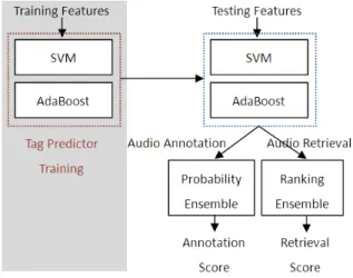
Fig. 1 shows the work flow of our audio tag annotation and retrieval system. We first split an audio clip into homogeneous segments, and then extract audio features with respect to vari- ous musical information, including dynamics, rhythm, timbre, pitch, and tonality, from each segment. The features in frame- based feature vector sequence format are further represented by their mean and standard deviation such that they can be combined with other segment-based features to form a fixed- dimensional feature vector for a segment. The prediction score for an audio clip given by a classifier is the average of the scores for its constituent segments. In the training phase, we train classifiers using our proposed cost-sensitive multi-label learning methods. In the testing phase, the classifiers output scores for audio tag annotation and retrieval, respectively.
Fig. 1. Work flow of the proposed audio tag annotation and retrieval system.
III. AUDIOSIGNALPROCESSING
For applying machine learning techniques to audio tag classification, we need to extract characteristic features of various types from the waveform of an audio clip by using some signal processing methods. Since feature selection is embedded in the training process of our classification method, we extract as many kinds of features as possible. However, for some frame-based features, such as Mel-frequency cepstral coefficients (MFCCs), we need to convert the variable-length feature vector sequence into a fixed-dimensional feature vector such that they can be used jointly with other features, like key and tempo. In this paper, the frame-based features are represented by their mean and standard deviation calculated over the audio clip (or segment as will be discussed later).
It is very likely that only a portion of the audio clip is associated with a specific tag. For instance, an audio clip may have the tag “female vocal” even though a female vocal only appears in the front part of the clip. Therefore, it might be inadequate to use the mean of MFCC vectors to represent the timbre of the whole clip. To solve this problem, we divide the
TABLE II
MUSICFEATURESUSED INTHISWORK
Category Feature Category Feature
Dynamics rms fluctuation peak
tempo Fluctuation fluctuation centroid
Rhythm attack time zero crossing rate
attack slope spectral flux
centroid low energy rate
spread Timbre MFCC
skewness delta MFCC
kurtosis delta-delta MFCC
entropy key clarity
Spectrum flatness key mode possibility
rolloff at 85% harmonic change
rolloff at 95% Tonality chromagram
brightness chroma centroid
roughness chroma peak
irregularity Pitch pitch value
clip into homogeneous segments and treat each segment as a unit in tag classification. Then, the final decision for the clip is based on the fusion of the results of its constituent segments.
A. Feature Extraction
To extract music features, we use MIRToolbox 1.13, a free software that comprises approximately 50 audio/music feature extractors and statistical descriptors [19]. As shown in Table II, we consider seven categories of features in this work, namely, dynamics, rhythm, spectrum, fluctuation, timbre, tonality, and pitch. We set default values for parameters in MIRToolbox, such as the length of window and hop size. After feature extraction, each clip (or segment) is represented by a 174- dimensional feature vector.
B. Audio Segmentation
Our audio segmentation is based on a measure of audio novelty proposed in [8]. We use the function implemented in MIRToolbox 1.1. An example segmentation result is shown in the bottom panel of Fig. 2. We first compute the cosine measure of MFCC vectors between any pairs of two frames in the audio clip, and build a self-similarity matrix, which can be visualized as a square image in the top panel of Fig.
2. The color scale of a pixel in the image is proportional to the similarity. Then, we can obtain a time-aligned novelty curve, as shown in the middle panel of Fig. 2, by convolving a checkerboard kernel with a radial Gaussian taper along the diagonal of the similarity matrix. The radial Gaussian taper of width H is defined as:
t(a, b) = exp{−4 × [(a − H/2
H/2 )2+ (b − H/2
H/2 )2]}, (1) where a, b = 1, 2, · · · , H, are the horizontal and vertical indexes of the Gaussian taper, respectively. Therefore, we only need to calculate a diagonal strip of width H when constructing the similarity matrix. In this paper, H is set to 64. Finally, the local peaks of the novelty curve, as marked by
3http://users.jyu.fi/∼lartillo/mirtoolbox/
circles in the middle panel of Fig. 2, are selected as segment boundaries. To prevent feature extraction and classification failures caused by insufficient data, we require the length of each segment to be at least 0.5 seconds.
Fig. 2. Illustration of audio segmentation.
IV. THEMIREX 2009 WINNINGMETHOD
In this section, we discuss our MIREX 2009 winning method. In the method, we assume the tags occur indepen- dently and do not consider the co-occurrences of tags. As a result, the tag classification problem is viewed as many independent binary classification problems, with a binary clas- sifier for each individual tag. For each tag, the final prediction combines the outputs of two classifiers: SVM and AdaBoost.
The tag count is transformed into 1 (with a tag) or 0 (without a tag) by using a threshold. Fig. 3 shows an overview of the classifier ensemble. It is used instead of the cost-sensitive multi-label classification in Fig. 1.
A. Support Vector Machine
SVM finds a separating surface with a large margin between training samples of two classes in a high-dimensional feature space implicitly introduced by a computationally efficient kernel mapping [20]. The large margin implies good gener- alization ability according to statistical learning theory. In this work, we exploit a linear SVM classifier f (x) of the following form:
f (x) = wTx + b. (2)
Given a training set (xi, yi)Ni=1 for a specific tag, where xi ∈ Rd is the feature vector of the i-th training sam- ple and yi ∈ {1, −1} is the class label, the parameters
Fig. 3. Work flow of the classifier ensemble used in the MIREX 2009 winning method.
w = (w1, w2, ..., wd) and b can be learned by solving a minimization problem formulated as follows:
w,b,ξmin
1
2wTw + CPN
i=1
ξi, s.t. yi(wTxi+ b) ≥ 1 − ξi
ξi ≥ 0
(3)
where ξi is the training error associated with instance xi; C is a tuning parameter that controls the tradeoff between maximizing the margin and minimizing the training error. The selection of C will be discussed in Section VIII.
B. AdaBoost
AdaBoost [21] finds a highly accurate classifier by com- bining several base classifiers, even though each of them is only moderately accurate. It has been successfully used in applications such as music classification [11] and audio tag classification [2]. The decision function of the AdaBoost classifier takes the following form:
f (x) = XT t=1
αtht(x), (4)
where ht(x) is the prediction score of a base classifier ht
given the feature vector x of a test sample; T is the number of base classifiers; and αtcan be calculated based on different versions of AdaBoost.
The base classifiers are learned iteratively. In the training phase, AdaBoost [22] maintains a weight vector Dt for the training instances in each iteration and uses a base learner to find a base classifier ht to minimize the weighted error according to Dt. In each iteration, the weight vector Dt is updated by
Dt+1(i) =Dt(i) exp(−αtyiht(xi))
Zt , (5)
where Ztis a normalization factor that makes Dt+1a distribu- tion. We can increase the number of base learners iteratively and stop the training process when the generalization ability on the validation set does not improve. We use a decision stump as the base learner in this study.
C. Ranking Ensemble
We noticed that the scales of the two classifiers’ prediction scores are rather different. Given a batch of testing clips, we first rank the prediction scores of individual classifiers independently. Then, the final score for a clip is the average of the ranks from the two classifiers. In this way, the smaller the average rank, the more likely the audio clip has the specific tag. We have applied this method in our MIREX 2009 submission. It achieves very good performance in terms of tag F-measure and tag AUC as these two metrics are more related to the ranking performance. However, the performance in terms of clip AUC is poor. In fact, this method is not suitable for the audio tag annotation task because it is unpractical to annotate a clip by referring to other clips simultaneously.
In order to annotate a single clip, we need to combine the scores from the two classifiers in a different way. Therefore, we propose probability ensemble instead of ranking ensemble for the audio tag annotation task.
D. Probability Ensemble
As each tag classifier is trained independently, the raw scores of different tag classifiers are not comparable. In the audio tag annotation task, we need to compare the scores of all tag classifiers and determine which tags should be associated with the given audio clip. Therefore, we transform the output score of SVM or AdaBoost into a probability score with a sigmoid function [23]:
P r(y = 1|x) ≈ 1
1 + exp(Af (x) + B), (6) where f (x) is the output score of a classifier on instance x, A and B are learned by solving a regularized maximum likelihood problem as suggested in [24]. As the classifier output has been calibrated into a probability score, a classifier ensemble is formed by averaging the probability scores of SVM and AdaBoost, and the probability scores of different tag classifiers become comparable.
V. TAGCOUNTSANDCOST-SENSITIVELEARNING
In this section, we describe our idea to improve the above MIREX 2009 winning method by treating the tag counts as costs and applying cost-sensitive learning. We first discuss several factors that affect the tag counts, and then introduce the concept of cost-sensitive learning.
A. Tag Counts
From our study of audio tagging websites, such as Last.fm and MajorMiner, we observe that certain factors affect the tag counts:
1) Consistent Agreement: Social tags are usually assigned by users (including malicious users) with different levels of musical knowledge and different intentions [1]. Tags may contain a lot of noisy information; however, when a large number of users consider that an audio clip should be associated with a particular tag, i.e., the count of the tag is high, the label information is deemed more
reliable. Conversely, if a tag is only assigned to an audio clip once, the annotation is considered untrustworthy. The MajorMiner website does not show such tags because they may contain noise. When training a classifier, using noisy label information can affect the generalization abil- ity of the classifier as discussed in Section I-A. Another problem that must be considered is that, sometimes, only a small portion of an audio clip is related to a certain tag.
For example, an instrument might only be played in the bridge section of a song. In this case, the count of the tag that corresponds to the instrument could be small.
2) Tag Bias: There are several types of audio tags, e.g., genre, instrumentation, mood, locale, and personal usage.
Some types (such as genre) are used more often than others (such as personal usage tags like “favorite” and
“I own it”); and specific tags (such as “British rock”) are normally used less often than general tags (such as
“rock”). In addition, audio tags typically contain many variants [1]. For example, on the Last.fm website “female vocalists” is a common tag, and “female vocals” and “fe- male artists” are variants of it. Fig. 4 shows the histogram of the average tag count estimated from MajorMiner data.
As mentioned earlier, the count of each tag is at least 2.
We observe that the average counts of most tags are close to 2.5. Some tags have higher average counts than the other tags. The top three most repeatedly assigned tags are “jazz”, “saxophone”, and “rap”; and the tags assigned least repeatedly are “drum machine”, “voice”, and “key- board.” We believe that repeatedly assigned tags describe acoustic characteristics that are easier to recognize (e.g.,
“drum machine” might easily be recognized as “drum”).
1.5 2 2.5 3 3.5 4 4.5 5 5.5
0 1 2 3 4 5 6 7 8 9 10
Number of tags
Average tag count
Fig. 4. Histogram of the average counts of tags on the MajorMiner website.
3) Song/Album/Artist Popularity: Popular songs, albums, and artists usually receive more tags, since people tend to tag music that they like or they are familiar with.
However, this is not the case for some web-based labeling games, such as MajorMiner, because the label flow can be controlled by the game designer. In addition, newly released songs usually receive fewer tags.
Based on the above observations, we formulate the audio tag annotation and retrieval task as a cost-sensitive classification
problem. In the next subsection, we examine the concept of cost-sensitive learning.
B. Cost-Sensitive Learning
Non-uniform misclassification costs are very common in a variety of pattern recognition applications, such as medical diagnosis, e-mail spam filtering, and business marketing. As a result, several cost-sensitive learning methods have been developed to address the problem, e.g., the modified learning algorithm [22] and the data re-sampling method [25]. Suppose we are given a cost-sensitive training set (xi, yi, ci)Ni=1 for a binary classification task, where ci⊂ [0, ∞) is the misclassifi- cation cost. The goal of cost-sensitive classification is to learn a classifier f (x) that minimizes the expected cost as follows:
E[cI(f (x) 6= y)], (7)
where I(·) is an indicator function that yields 1 if its argument is true, and 0 otherwise. The expected cost-insensitive cost is defined as:
E[I(f (x) 6= y)], (8)
which is a special case of (7) where all samples have an equal misclassification cost c.
To formulate the audio tag prediction task as a cost- sensitive classification problem, we minimize the total counts of misclassified tags by treating the tag counts as costs. In other words, our goal is to correctly predict the most frequently used tags, such as tags of consistent agreement, popular tags, and the tags for popular songs/albums/artists. For example, consider the first audio clip from the song Hi-Fi in Table I and suppose a tag prediction system A only predicts the tag “drum”
correctly, while another tag prediction system B predicts two tags “electronic” and “beat” correctly. We consider that system A outperforms system B because the tag count of “drum” is more than the sum of the other two tags of this audio clip.
Both SVM and AdaBoost can be extended to the cost- sensitive versions to solve the cost-sensitive binary classifi- cation problem. Cost-sensitive SVM can be learned by modi- fying (3) to
w,b,ξmin
1
2wTw + CPN
i=1
ciξi, s.t. yi(wTxi+ b) ≥ 1 − ξi
ξi ≥ 0
(9)
where each cost ciis associated with a corresponding training error term ξi. Cost-sensitive AdaBoost [22] can be learned by modifying the update rule of weight vector Dtin (5) to
Dt+1(i) = Dt(i) exp(−αtciyiht(xi))
Zt , (10)
where ci is the cost of training instance xi.
However, cost-sensitive binary classification still assumes the tags are independent and loses the co-occurrence infor- mation of tags. Therefore, we propose using cost-sensitive multi-label classification for the audio tagging task in the next section.
VI. COST-SENSITIVEMULTI-LABELCLASSIFICATION
We first introduce the concept of multi-label classification.
Let x ∈ Rd, which is a d-dimensional input space, and Y ⊆ L = {1, 2, ..., K}, which is a finite set of K possible labels.
To facilitate the discussion, hereafter, Y is represented by a vector y = (y1, y2, ..., yK) ∈ {1, −1}K. Given a training set (xi, yi)Ni=1 that contains N samples, the goal of multi-label classification is to learn a classifier h : Rd → 2L such that h(x) predicts which labels should be assigned to an unseen sample x.
Cost-sensitive multi-label classification extends multi-label classification by coupling a cost vector ci ∈ RK to each training sample (xi, yi). The j-th component cij denotes the cost to be paid when the label yij is misclassified. More specifically, cij is a false negative cost when yij = 1, and a false positive cost when yij = −1. In this work, the false negative cost is set as the tag count while the false positive cost is uniformly set to one. We extend two existing multi- label learning algorithms, namely, stacking [17] and RAkEL [18], to solve the CSML problem.
A. Cost-Sensitive Stacking
Stacking is a method of combining the outputs of multiple independent classifiers for multi-label classification. Assume that the K tags are independent and their tag classifiers are trained independently. The first step of using stacking for multi-label classification is to use the outputs of all classifiers, f1(x), f2(x), ..., fK(x), as features to form a new feature set.
Let the new feature be z = (z1, z2, ..., zK). Then, we can use the new feature set together with the true label to learn the parameters wkj of the stacking classifiers:
hk(z) = XK j=1
wkjzj, (11)
where the weight wkj will be positive if tag j is positively correlated to tag k; otherwise, wkj will be negative. The stacking classifiers can recover misclassified tags by using the correlation information captured in the weight wkj.
Inspired by the idea of stacking, we improve our MIREX 2009 classifier ensemble by using cost-sensitive stacking.
As shown in Fig. 5, we first train K SVM-based and K AdaBoost-based cost-sensitive binary tag classifiers by using the tag counts as costs independently. Then, we use stacking SVM to respectively process the outputs of the SVM-based binary tag classifiers and the outputs of the AdaBoost-based binary tag classifiers. Note that the stacking SVM itself is cost-insensitive. Finally, we apply the ranking ensemble or probability ensemble method.
B. Cost-Sensitive RAkEL
Label powerset (LP) method is a major category of multi- label learning algorithms. It reduces the multi-label classi- fication problem to a single-label multi-class classification problem by treating each distinct combination of labels in the training set as a different class. It is computationally more efficient than treating the multi-label classification problem
Fig. 5. Work flow of the cost-sensitive stacking-based audio tag annotation and retrieval system.
as several binary classification problems. However, when the number of labels increases, the number of classes increases exponentially, and each class will be associated with very few training instances.
In [18], a method called Random k-Labelsets is proposed to realize the LP method. A k-labelset is a labelset R ⊆ L with
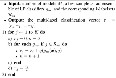
|R| = k. RAkEL randomly selects a number of k-labelsets from L and uses the LP method to train the correspond- ing multi-label classifiers. Algorithms 1 and 2 describe the training and classification processes of RAkEL, respectively.
The prediction of a multi-class LP classifier gm for sample x is denoted by gm(x) ∈ {1, 2, . . . , V }. Note that V will be much smaller than 2k if the data is sparse. In Algorithm 2, q(gm(x), j) is defined as:
q(gm(x), j) =
1 j ∈ Rm and j is positive in gm(x),
−1 j ∈ Rm and j is negative in gm(x),
∅ j /∈ Rm.
(12) For example, when k = 2, the classes 1, 2, 3, and 4 correspond to (1, 1), (1, −1), (−1, 1), and (−1, −1), respectively. If tag j is not included in Rm, q(·, j) is undefined. If tag j corresponds to the first label of Rm, q(1, j), q(2, j), q(3, j), and q(4, j) will output scores 1, 1, −1, and − 1, respectively.
In order to use the tag counts as misclassification costs, we extend RAkEL for cost-sensitive multi-label classification.
The extension is not straightforward since we are given a cost value for each label but RAkEL considers a set of labels as a class. Our idea is to train the cost-sensitive LP classifier ˆ
gm by transforming the cost of each label in a labelset to the total cost of the labelset. The transformed cost ˆciof a training
Algorithm 1 The training process of RAkEL
• Input: number of models M , size of labelset k, set of labels L, and the training set D = (xi, yi)Ni=1
• Output: an ensemble of LP classifiers gmand the corre- sponding k-labelsets Rm
1) Initialize S ← Lk
2) for m ← 1 to min(M ,|Lk|) do
• Rm← a k-labelset randomly selected from S
• train the LP classifier gmbased on D and Rm
• S ← S \ Rm
3) end
Algorithm 2 The classification process of RAkEL
• Input: number of models M , a test sample x, an ensem- ble of LP classifiers gm, and the corresponding k-labelsets Rm
• Output: the multi-label classification vector r = (r1, r2, ..., rK)
1) for j ← 1 to K do a) rj = 0, n = 0
b) for each gm, if j ∈ Rmdo
• rj = rj+ q(gm(x), j)
• n = n + 1 c) end
d) rj= rnj 2) end
sample xi for training ˆgmis computed by
ˆci(ci, yi) =
( P
j∈Rms.t. yij=1
cij if ∃j ∈ Rm s.t. yij = 1,
1 else,
(13) where ci is the cost vector mentioned in the beginning of Section VI. Therefore, we can obtain the multi-class training sample with the associated cost, (xi, ˆyi, ˆci), for training the LP classifier, where ˆyi∈ {1, 2, . . . , V } is the class value and ˆci is the cost to be paid when the class of this instance is misclassified. We use the multi-class SVM as the LP classifier in this study, and employ the one-versus-one strategy [26] in cost-sensitive multi-class classification. In the experiments, we will compare RAkEL with cost-sensitive RAkEL.
VII. COST-SENSITIVEEVALUATIONMETRICS
The evaluation metrics used at MIREX 2009, namely, the accuracy, tag F-measure, tag AUC, and clip AUC, did not consider the costs (i.e., tag counts). Moreover, the class distribution of each binary tag classification problem was imbalanced. For example, in the MajorMiner dataset used at MIREX 2009, out of the forty-five tags, only twelve had more than 10% positive instances. Using accuracy as the evaluation metric biases the system towards the negative class. Since these metrics do not take the costs into account, we propose three cost-sensitive metrics. First, we define the cost-sensitive
precision (CSP) and the cost-sensitive recall (CSR) as follows:
CSP = Weighted Sum of TP
Weighted Sum of TP+Weighted Sum of FP, (14)
CSR = Weighted Sum of TP
Weighted Sum of TP+Weighted Sum of FN, (15) where TP, FP, and FN denote the true positive, the false positive, and the false negative, respectively. The weight of each positive instance is assigned as the count of the associated tag. However, assigning a weight to each negative instance is not as straightforward because people do not use negative tags like “non-rock” and “no drum.” Therefore, we assign a uniform cost to negative instances and balance the cost between positive and negative classes, i.e., the total cost of the positive instances is the same as that of the negative instances.
As a result, the expected CSP of a random guess baseline method will be 0.5. Then, we can define cost-sensitive metrics based on CSP and CSR.
The cost-sensitive F-measure can be calculated as follows:
2 × CSR × CSP
CSR + CSP . (16)
The receiver operating characteristic curve is a graphical plot of the true positive rate (recall) versus the false positive rate as the decision threshold varies. The AUC is often used to eval- uate a binary classifier’s performance on a class-imbalanced dataset. We can modify the AUC to obtain a cost-sensitive AUC by replacing the recall metric with CSR. Then, we use the cost-sensitive clip AUC and the cost-sensitive tag AUC to evaluate the audio tag annotation task and the audio tag retrieval task, respectively.
VIII. MIREX 2009 RESULTS
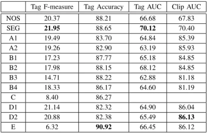
The submissions to the MIREX 2009 audio tag classification task have been evaluated on two datasets: the MajorMiner set and the mood set [27]. The algorithms were evaluated with three-fold cross validation and artist filtering was used in the production of the test and training splits. The evaluation metrics include the tag F-measure and tag AUC. Both metrics correspond to the tag retrieval task that is aimed at retrieving audio by a given tag query. The metrics also include clip AUC and the tag accuracy. These two metrics correspond to the tag annotation task that is aimed at annotating a given audio clip with correct tags.
The results of evaluation on the two datasets are summarized in Tables III and IV, respectively. The best result of each specific evaluation metric is bold-typed. The names in the first column indicate the twelve submissions. Our submissions without and with pre-segmentation are denoted by NOS and SEG, respectively. It is clear that pre-segmentation is effective.
Table V summarizes the ranking of our two submissions in terms of the four evaluation metrics on the two datasets. Our SEG submission achieves the best performance in terms of the metrics corresponding to the audio tag retrieval task (i.e., tag F-measure and tag AUC) but performs poorly in terms of the metric corresponding to the audio tag annotation task (i.e.,
TABLE III
EVALUATIONRESULTS OFMIREX 2009 AUDIOTAGCLASSIFICATION ON THEMAJORMINERDATASET. THERE ARE12SUBMISSIONS. OUR SUBMISSIONS WITHOUT AND WITH PRE-SEGMENTATION ARE DENOTED BY
NOSANDSEG,RESPECTIVELY
Tag F-measure Tag Accuracy Tag AUC Clip AUC
NOS 28.90 90.01 78.22 75.14
SEG 31.08 90.35 80.73 77.37
A1 27.68 86.78 74.18 87.08
A2 28.99 85.95 76.14 86.13
B1 20.93 91.22 76.16 88.24
B2 24.14 90.51 79.07 88.23
B3 17.05 91.32 72.11 85.45
B4 26.26 88.95 74.85 85.45
C 1.22 89.08
D1 29.00 85.02 78.39 87.24
D2 29.34 85.05 78.62 87.63
E 4.43 91.44 73.64 85.11
TABLE IV
EVALUATIONRESULTS OFMIREX 2009 AUDIOTAGCLASSIFICATION ON THEMOODDATASET. THERE ARE12SUBMISSIONS. OUR SUBMISSIONS
WITHOUT AND WITH PRE-SEGMENTATION ARE DENOTED BYNOSAND SEG,RESPECTIVELY
Tag F-measure Tag Accuracy Tag AUC Clip AUC
NOS 20.37 88.21 66.68 67.83
SEG 21.95 88.65 70.12 70.40
A1 19.49 83.70 64.84 85.39
A2 19.26 82.90 63.19 85.93
B1 17.23 87.77 65.18 84.85
B2 17.98 88.15 68.12 84.85
B3 14.71 88.22 62.88 81.18
B4 18.33 86.17 64.60 81.19
C 8.40 86.27
D1 21.14 82.32 64.90 86.04
D2 20.88 82.38 65.49 86.13
E 6.32 90.92 66.45 86.12
clip AUC). The details about the evaluation datasets and the other submissions are available on the MIREX website4.
IX. EXTENDEDEXPERIMENTS
This section presents the results of extended experiments on the downloaded MajorMiner dataset. We extensively evaluate
4http://www.music-ir.org/mirex/wiki/2009:MIREX2009 Results
TABLE V
PERFORMANCERANKINGS OFOURTWOSUBMISSIONS TOMIREX 2009 AUDIOTAGCLASSIFICATION ONTWODATASETS
Evaluation Ranking
Metrics SEG NOS
Tag AUC 1 5
The MajorMiner Tag F-measure 1 5
Dataset Clip AUC 11 12
Tag Accuracy 5 6
Tag AUC 1 3
The Mood Tag F-measure 1 4
Dataset Clip AUC 11 12
Tag Accuracy 2 3
TABLE VI
THE45 TAGSUSED INTHEMIREX 2009 AUDIOTAGCLASSIFICATION EVALUATION
metal instrumental horns piano guitar
ambient saxophone house loud bass
fast keyboard electronic noise british
solo electronica beat 80s dance
jazz drum machine strings pop r&b
female rock voice rap male
slow vocal quiet techno drum
funk acoustic distortion organ soft
country hip hop synth trumpet punk
the individual classifiers, the ranking ensemble method, the probability ensemble method, and the CSML methods.
A. Dataset
Our extended experiments basically follow the MIREX 2009 setup. The evaluation data come from the MajorMiner’s music labeling game5, which invites players to listen to short music clips (each about 10 seconds long) and label them with relevant words and phrases. According to the MIREX 2009 audio tag classification result web page, 45 tags, as listed in Table VI, are considered. We download all the audio clips that are associated with these 45 tags from the website of the MajorMiner’s game. The resulting audio database contains 2,472 clips and the duration of each clip is 10 seconds or less. The dataset might be slightly different from that used in MIREX 2009 because the MajorMiner website might have been updated recently.
B. Model Selection and Evaluation
We adopt three-fold cross-validation in the experiments following the evaluation method at MIREX 2009. The 2,472 clips are randomly split into three subsets. In each fold, one subset is selected as the test set and the remaining two subsets serve as the training set. The test set for (outer) cross- validation is not used for determining the classifier setting.
Instead, we first perform inner cross-validation on the held out data from the training set to determine the cost parameter C in SVM and the number of base learners in AdaBoost. Then, we re-train the classifiers with the complete training set and the selected parameters, and perform outer cross-validation on the test set. Since the class distributions for some tags are imbalanced (more than two thousand negative instances and less than fifty positive instances), classification accuracy is not a fair criterion for model selection. Therefore, we use the tag AUC as the model selection criterion. For RAkEL and its cost- sensitive version, the number of models, M , is set to 250, and the size of the labelset, k, is set to 14.
To calculate the tag F-measure and tag accuracy, we need a threshold to binarize the output score. For the audio tag retrieval task, we want to retrieve audio clips from the audio database. We assume that each tag’s class has similar proba- bility distributions in the training and testing audio databases.
5http://majorminer.org/
Therefore, we set the threshold to select relevant audio clips according to the class prior distribution obtained from the training data. For the audio tag annotation task, we annotate the testing audio clips one by one. We set the threshold to 0.5 because the calibrated probability score ranges from 0 to 1.
C. Experimental Results
Our experimental results in terms of the metrics correspond- ing to the audio tag annotation task and the audio tag retrieval task are summarized in Table VII. Because the cross-validation split used in MIREX 2009 is not available, we perform three- fold cross-validation twenty times and calculate the mean and standard deviation of the results of different cross-validation splits.
Several observations can be drawn from Table VII. First, pre-segmentation is effective. All the classification methods benefit from pre-segmentation. For example, the tag AUC is improved by 1.42% (cf. SVM) and 4.23% (cf. AdaBoost).
Second, SVM slightly outperforms AdaBoost. Third, the two ensemble methods are respectively suitable for either the retrieval task or the annotation task as discussed above. On the audio tag retrieval task, ranking ensemble not only has better mean performance than any individual classifier, but also has a smaller standard deviation. Probability ensemble is more suitable than ranking ensemble for the audio tag annotation task. However, the improvement over the SVM classifier is small.
Next, we compare the CSML methods, which exploit the tag count and correlation information jointly, with the MIREX 2009 winning method. We also evaluate the cost- sensitive binary classification (CS only) methods and the cost- insensitive multi-label (ML only) classification methods. We perform three-fold cross-validation one hundred times and calculate the mean and standard deviation of the results. The experimental results in terms of the cost-sensitive metrics and regular metrics are summarized in Tables VIII and IX, respectively. The AdaBoost-, SVM-, and Ensemble-MIREX methods are the same as that used in Table VII. The Ensemble methods use probability ensemble to generate Clip AUC and ranking ensemble to generate F-measure and Tag AUC. For the AdaBoost, SVM, and Ensemble methods, the ML only method employs stacking, and the CSML method employs cost-sensitive stacking. The cost-sensitive RAkEL method is compared to its cost-insensitive version.
The results in Table VIII demonstrate the effectiveness of CSML learning. The improvement in the cost-sensitive F- measure is the most significant: 3.87% for AdaBoost-CSML versus AdaBoost-MIREX, 3.66% for SVM-CSML versus SVM-MIREX, 2.27% for Ensemble-CSML versus Ensemble- MIREX, and 1.07% for cost-sensitive RAkEL (i.e., RAkEL- CSML) versus RAkEL (i.e., RAkEL-ML only). The cost- sensitive stacking methods outperform their cost-insensitive binary classification counterparts in terms of all evaluation metrics (cf. AdaBoost-CS only versus AdaBoost-MIREX and AdaBoost-CSML versus AdaBoost-ML only). However, cost- sensitive RAkEL is slightly worse than RAkEL in terms of cost-sensitive Clip AUC and Tag AUC, although the difference
TABLE VIII
AUDIOTAGANNOTATION ANDRETRIEVALRESULTS OFCOST-SENSITIVE MULTI-LABELCLASSIFICATIONMETHODS INTERMS OFCOST-SENSITIVE
METRICS(IN%)
Mean CS CS CS
Classifier ±St.d. Clip AUC F-measure Tag AUC MIREX 88.92±0.09 41.04±0.65 80.53±0.24 CS Only 89.67±0.07 44.71±0.58 81.74±0.21 AdaBoost ML Only 89.60±0.11 42.71±0.68 80.97±0.32 CSML 89.88±0.09 44.91±0.62 81.79±0.29 MIREX 89.47±0.09 43.95±0.56 81.22±0.28 CS Only 90.08±0.06 45.92±0.56 82.20±0.20 SVM ML Only 90.08±0.08 45.49±0.51 82.53±0.20 CSML 90.67±0.07 47.61±0.63 83.11±0.23 MIREX 89.65±0.07 46.04±0.57 83.03±0.19 CS Only 90.32±0.06 47.94±0.61 83.63±0.18 Ensemble ML Only 90.21±0.07 46.65±0.56 83.45±0.18 CSML 90.61±0.06 48.31±0.62 83.89±0.17 ML Only 91.11±0.08 45.57±0.59 84.77±0.12 RAkEL CSML 90.97±0.09 46.64±0.61 84.13±0.16
is not significant. From the table, we observe that both the CS only methods and the ML only methods are effective and the CS only methods are slightly better than the ML only methods.
We also observe that the standard deviations of the results are very small.
TABLE IX
AUDIOTAGANNOTATION ANDRETRIEVALRESULTS OFCOST-SENSITIVE MULTI-LABELCLASSIFICATIONMETHODS INTERMS OFREGULAR
(COST-INSENSITIVE) METRICS(IN%)
Mean
Classifier ±St.d. Clip AUC F-measure Tag AUC MIREX 87.73±0.09 30.27±0.46 79.41±0.25 CS Only 88.54±0.07 32.20±0.41 80.56±0.20 AdaBoost ML Only 88.50±0.11 31.18±0.45 79.91±0.31 CSML 88.82±0.09 32.42±0.45 80.69±0.28 MIREX 88.29±0.10 31.77±0.37 80.01±0.27 CS Only 88.96±0.06 32.93±0.38 81.12±0.20 SVM ML Only 89.00±0.08 32.70±0.36 81.41±0.19 CSML 89.64±0.07 34.22±0.41 82.06±0.23 MIREX 88.47±0.07 33.35±0.40 81.89±0.19 CS Only 89.21±0.06 34.32±0.41 82.54±0.18 Ensemble ML Only 89.12±0.07 33.59±0.37 82.37±0.18 CSML 89.57±0.06 34.69±0.46 82.85±0.17 ML Only 88.67±0.10 33.41±0.41 79.15±0.22 RAkEL CSML 89.63±0.10 33.84±0.40 81.41±0.22
Table IX compares the results of different methods in terms of the regular (cost-insensitive) evaluation metrics. Interest- ingly, the cost-sensitive stacking methods outperform their cost-insensitive binary classification counterparts in terms of the regular metrics (cf. AdaBoost-CS only versus AdaBoost- MIREX and AdaBoost-CSML versus AdaBoost-ML only).
Recall that tags with smaller counts may contain noisy labeling information. By viewing the tag counts as costs, the cost- sensitive learning method can ignore the noisy information by giving a smaller penalty (cost), and thereby train a more accurate classifier. Moreover, cost-sensitive RAkEL outper- forms RAkEL in terms of all three metrics, and is better than