國立臺灣大學生物暨農學院農藝學研究所 生物統計學組碩士論文
Division of Biometry Graduate Institute of Agronomy College of Bioresources and Agriculture
National Taiwan University Master thesis
生物相似性藥品之設限資料 對等性評估的研究
A Study for Application of the Parallel-line Assay to Evaluation of Biosimilar Drug Products
Based on Censored Data
張育誠Yu-Cheng Chang
指導教授﹕劉仁沛 博士
Advisor: Jen-Pei Liu, PH.D.
中華民國 102 年 6 月 June, 2013
i
ii
謝辭
首先誠摯的感謝指導教授劉仁沛博士,老師悉心的教導使我得以一窺統計 於製藥領域的深奧,不時的討論並指點我正確的方向,使我在這兩年中獲益匪淺。
老師對學問的嚴謹更是我輩學習的典範。
本論文的完成得感謝張智熙學長與林亞靚學姐的大力協助。因為有兩位的幫 忙,使得本論文能夠更完整而嚴謹。兩年裡的日子,實驗室里共同的生活點滴,學 術上的討論、言不及義的閒扯、因為睡太晚而遮遮掩掩閃進教室...,各位的陪伴 讓兩年的研究生活變得絢麗多彩。感謝志榮學長、姜杰學長不厭其煩的指出我研究 中的缺失,且總能在我迷惘時為我解惑,也感謝亭甄同學、松林同學、智揚同學的 幫忙,恭喜我們順利走過這兩年。實驗室的楊宇晴學妹、姚力維學弟與黃証群學弟 當然也不能忘記,你/妳們的幫忙及搞笑我銘感在心。
最後要再次謝謝劉仁沛老師,你的處處諒解真的讓我十分感動,我一直是個有 話不敢說的人。很多時候自己內心無法給自己答案,就會想要放棄一切。在我最低 落的時候總會感受到老師的幫助,雖然我不常找老師聊天,但是在各種小地方上都 可以感受到老師對我們的照顧,我非常感動。除了感謝外我也必須道歉,我真的一 直給老師添麻煩了。
張育誠 台灣大學農藝所生物統計組 民國 102 年 6 月
iii
English Abstract
In recent years, biologics market of biological drug increases rapidly, but the development costs are also very high. Therefore, after the patent of biological products expires, many pharmaceutical companies have invested in the development of biosimilar products. But, biological products, with process specificity, are different from traditional small molecule drug products. Therefore the methods for assessment of biosimilar products are also different from that of chemical generic products. Current regulations indicate that the clinical trials for assessment can be waived on a case-by-case basis, but a pharmacovigilance is necessary. However, if the requirement for clinical trials cannot be waived, the development cost of biosimilar products will be the same as that of the innovators. It cannot achieve the goal of cost reduction, and deny of access of biological drug products to needed patients.
In this thesis, we propose to apply the parallel-line assay to test whether the approval of the biosimilar products should require clinical trials. We developed the statistical
testing procedure to evaluate the equivalence between the biosimilar drug product and innovator’s biological procedure when the primary endpoint is a censored variable which
follows an exponential distribution. The results of size and power from the simulation studies are presented. A numerical example is used to illustrate the application of the
iv
proposed method
Keywords: Biological products, Biosimilar, Censored endpoints, Exponential distribution.
v
中文摘要
生物製劑的市場近年來逐漸增加,但是所需的開發成本仍然很高,所以在生 物製劑的專利到期以後,許多藥廠紛紛投入生物相似性藥品的研發。不同於一般 的化學分子學名藥,生物製劑具有製程專一的特性,所以評估生物相似性藥品必 須與化學分子學名藥有所不同。現行法規中,生物相似性藥品需依個案,適度的 減免臨床試驗,才能被核准上市,成本並不小於開發新的生物製劑,無法降低成 本,達到造福病患之目的。
當療效指標為設限資料時,本篇論文以對數風險率回歸檢定法評估生物製劑 相似性藥品與原廠生物製劑是否為相似,以評估是否需要執行完整臨床試驗,模 擬所提出方法之第一型錯誤機率、檢定力和覆蓋率,並以數值例子來介紹方法之 應用。
關鍵字: 生物製劑,生物製劑相似性藥品,設限資料,指數分佈。
vi
Contents
Chapter 1 Introduction ... 1
1.1 Background and Motivations ... 1
1.2 Bioequivalence and Regulations ... 3
1.3 Aims of the study ... 6
Chapter 2 Literature Review ... 10
2.1 Interval Hypotheses ... 10
2.2 Biological Assay ... 12
2.3 Parallel Line Assay to Evaluation of the Similarity of Biosimilar Products ... 13
2.4 Survival Analysis ... 16
2.4 Log-hazard Linear Regression Model. ... 21
2.5 Newton-Raphson Method ... 24
Chapter 3 Proposed Methods ... 28
3.1 Design ... 28
3.2 The Procedure and Methods Based on Relative Potency of Product Characteristics .. 30
3.2.1 Test for Parallelism of Log-hazard Regressions ... 32
3.2.2 Estimate Relative Potency and Its Confidence Interval ... 36
Chapter 4 A Numerical Example ... 39
Chapter 5 Simulation Studies ... 49
5.1 Selection of Dose Levels ... 49
5.2 Simulation Processes ... 51
5.3 Simulation Results ... 52
Chapter 6 Discussions and Conclusions ... 69
References 71 Appendix 1, Fortran Codes for Numerical Example ... 74
Appendix 2, Fortran Codes for Selection of Dose Levels Program ... 84
Appendix 3, Fortran Code for Simulation Program ... 95
vii
List of Tables
Table1.2: The differences between small-molecule generics and biosimilar products. ... 9
Table 4.1: The dose levels and the hazard rate of the censored responses of the numerical example ... 44
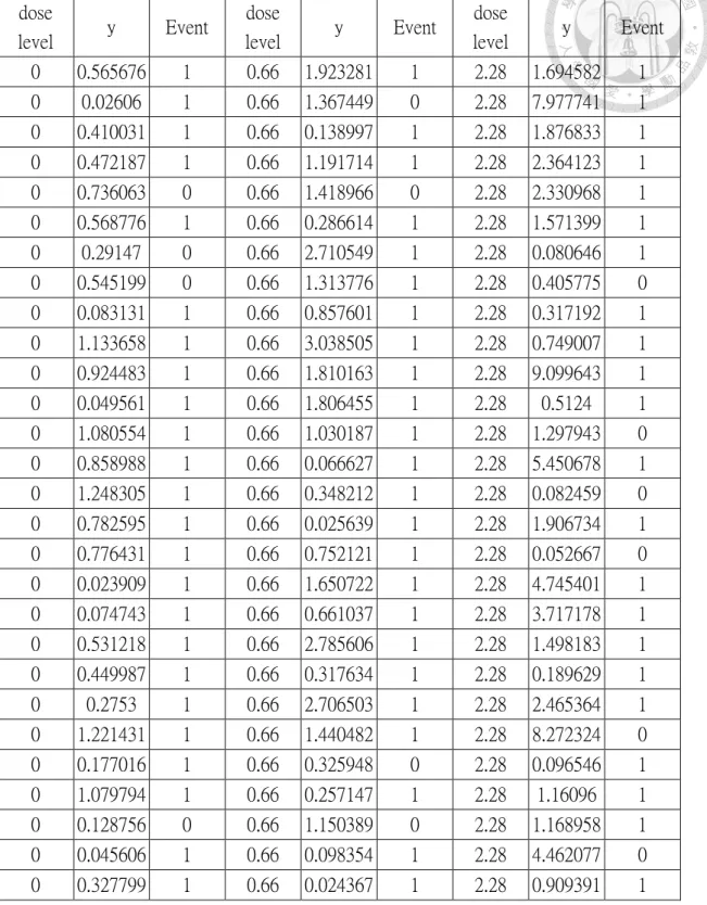
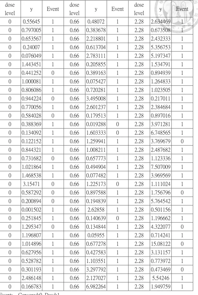
Table 4.2: The data of innovator's product of the numerical example ... 45
Table 4.2: The data of innovator's product of the numerical example (continued) ... 46
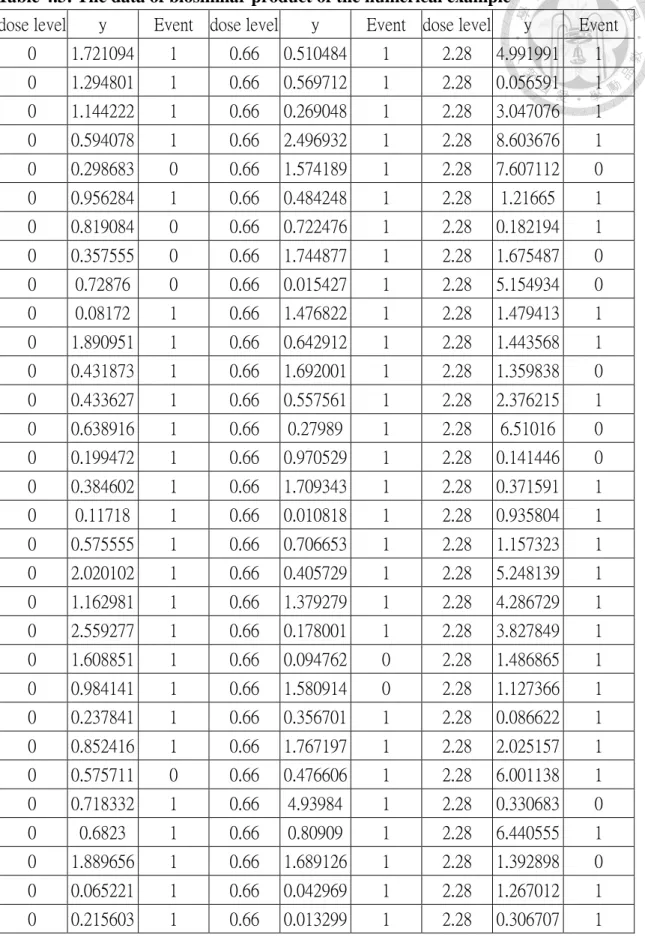
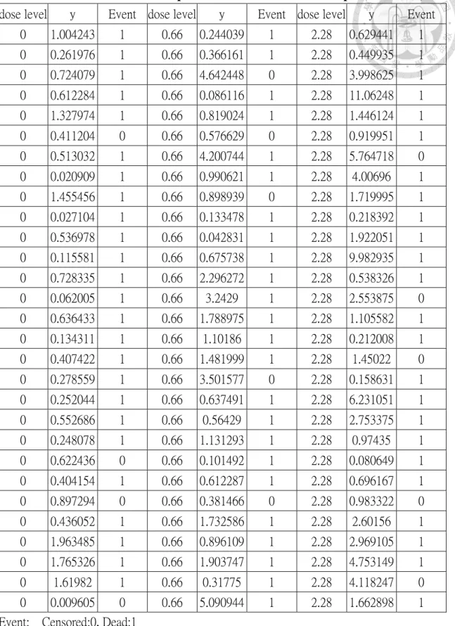
Table 4.3: The data of biosimilar product of the numerical example ... 47
Table 4.3: The data of biosimilar product of the numerical example (continued) ... 48
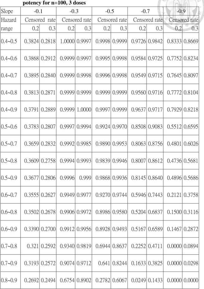
Table 5.1: The results of empirical power for selection of doses based on relative potency for n=100, 3 doses ... 55
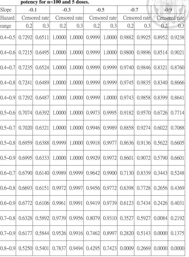
Table 5.2: The results of empirical power for selection of doses based on relative potency for n=100 and 5 doses. ... 56
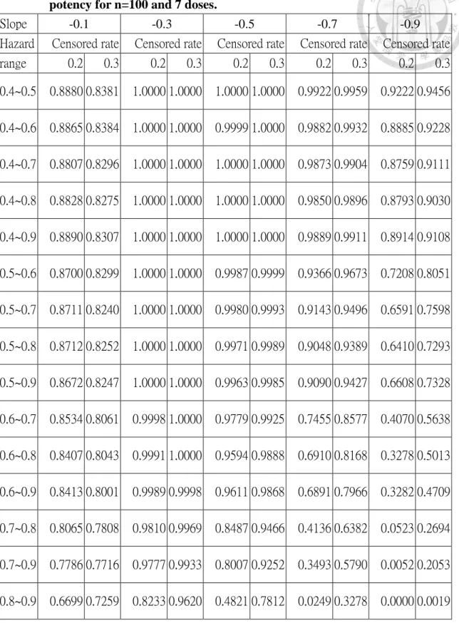
Table 5.3: The results of empirical power for selection of doses based on relative potency for n=100 and 7 doses. ... 57
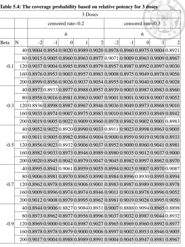
Table 5.4: The coverage probability based on relative potency for 3 doses ... 58
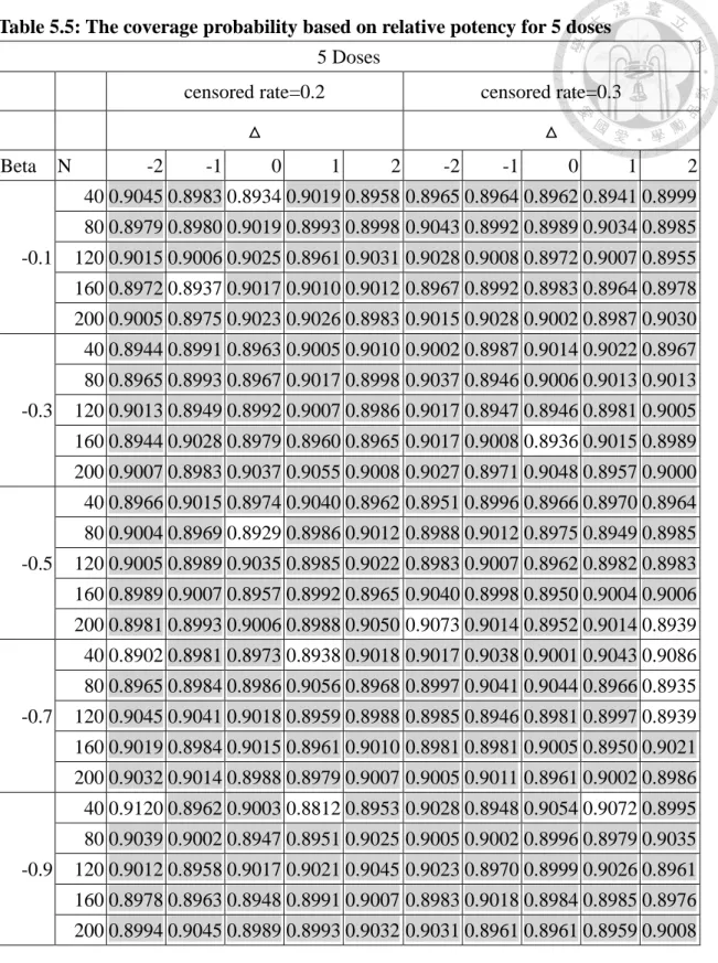
Table 5.5: The coverage probability based on relative potency for 5 doses ... 59
Table 5.6: The coverage probability based on relative potency for 7 doses ... 60
Table 5.7: A summary of coverage probabilities ... 61
Table 5.8: The empirical size and empirical power based on relative potency for 3 doses 62 Table 5.9: The empirical size and empirical power based on relative potency for 5 doses 63 Table 5.10: The empirical size and empirical power based on relative potency for 7 doses ... 64
Table 5.11: A summary of empirical sizes. ... 65
viii
List of Figures
Figure 2.1: Design (a) for evaluation of extrapolation ability ... 27 Figure 5.1: Flow chart of selection of dose levels ... 66 Figure 5.2: Flow chart of simulation process ... 67 Figure 5.3: The empirical power curve when the slope =-0.3, doses = 3 ,censored rate =
0.3 and n = 40. ... 68
1
Chapter 1 Introduction
1.1 Background and Motivations
Biologics are therapeutic moiety manufactured by a living system or organism, such as human, plants, animals or microorganisms, and they are used for medical, prevention and cure of human diseases. It can be applied to cancer, diabetes mellitus, growth impairment, and many other diseases. Furthermore, biologics include a wide range of medicinal products such as vaccines, blood and blood components, somatic cells, gene therapy, tissues, and recombinant therapeutic proteins created by biological processes.
Biologics are important life-saving drug products for patients with insufficiently medical needs. The worldwide sales of biologics in 2008 reached US $125 billion dollars which accounts about 20% of the pharmaceutical industry.
In addition, unlike the chemical drug products, biological products, which are much larger molecular weights, can be composed of sugars, proteins, or nucleic acids or complex combinations of these substances, or may be living entities such as cells and tissues. In short words, biological products are organic compounds made of amino acids, which possess primary, secondary, tertiary and quaternary structures. Biologic products are sensitive to heat, light, and shock, and it can easily be contaminated by manufacturing
2
process changes. Therefore, the manufacture of biological agents has to be noted, such as types of bacteria, the cells to create the protein and the quality of production equipments.
Therefore the biological products are very expensive and can reach up to US $ 120,000 per patient per year. This high cost denies the accessibility of most of patients to the most of life-saving biological products. (Webber, 2007, Wikipedia, Biosimilar and Biologic, 2011.04)
Many best-selling biological products will face patent expiration in recent years.
Table 1.1 shows that several biological products have reached the end of their patent protection. Therefore, generic reproductions of the innovator’s biological products can be made available. These generic reproductions of the innovator’s biological products are called biosimilar products by the European Union and follow-on biologics in the United States. In 2008, the US Congressional Budget Office predicted a savings of US $25 billion dollars in the next 10 years. Because of reduction of unnecessary drug testing and clinical trials, the price of the biosimilar drug products can be reduced and become affordable for most needed patients.
Biosimilars or follow-on biologics are not like the common small-molecule chemical drugs. Biologics generally exhibit high molecular complexity and may be quite sensitive to manufacturing process changes. Table 1.2 provides comparisons of the differences between small-molecule chemical generics and biosimilar products. Therefore,
3
assessment of biosimilar products may also be different. The innovators of the biological products suggest that biosimilar products should not be approved without data from large clinical trials. However if approved of biosimilar products requires clinical trials, then development cost of biosimilar products will be the same as that of the innovators. As a result, it cannot achieve the goal of cost reduction to benefit the patients.
Liu and Chow (2010) suggest that applying the method of parallel line assay to verify whether the clinical trials are required for approval of the biosimilar products and to assess the equivalence between the innovator and biosimilar products if validated characteristics of the drug products are reliable predictors of clinical responses. 林亞靚
(2010) proposed to apply the parallel line assay to the quantitative and continuous responses, 張 志 熙 (2011) proposed to apply the parallel line assay to the binary
responses. Simulation results of both methods can adequately control the size.
1.2 Bioequivalence and Regulations
For small molecular chemical compounds, measures of bioavailability include the peak concentration (Cmax) and the area under the concentration – time curve (AUC). The assessments of traditional chemical generic drugs are based on pharmacokinetics measures and the approval of traditional chemical generic drugs is based on the following Fundamental Bioequivalence Assumption (Chow and Liu, 2010)
4
When two drug products are equivalent in the rate and extent to which the active drug ingredient or therapeutic moiety is absorbed and becomes available at the site of drug action, it is assumed that they will be therapeutically equivalent and can be used interchangeably.
Next, we briefly review the regulations for approval of the traditional chemical generic drug products of small molecules.
Europe
According to the European regulations, two medicinal products are bioequivalent if they are pharmaceutically equivalent or pharmaceutical alternatives and if their bioavailability after administration in the same molar dose is similar to such a degree that their effects, with respect to both efficacy and safety, will be essentially the same. This can be demonstrated if the 90% confidence intervals of the means ratios between the two preparations based on Cmax and AUC lie in the range of (0.80, 1.25) or (-0.2231, 0.2231) for the log-transformed data. (EMEA, 2001)
United States
The FDA considers two products are bioequivalent if based on Cmax, AUC(0-t) and AUC(0-∞), the 90% CI of the ratio of the means of the test (e.g. generic formulation) to the reference (e.g. innovator brand formulation) is within 80.00% to 125.00%. (US FDA, 2001 and 2003)
Taiwan
5
The Department of Health of Taiwan also has similar regulations for approval of
generic products with respect to Cmax, AUC(0-t) and AUC(0-∞) based on the logarithm scale.
If the 90% confidence interval of the mean ratio between generic and innovator of products is within (0.8, 1.25), then the generic drug product is claimed to the bioequivalent to the innovator’s drug product. (TFDA, Taiwan, 2009)
Since approval of the traditional chemical generic drugs does not require conducting expensive and large clinical trials, the costs of chemical generic drugs are quite inexpensive, usually 1/5 to 1/2 of the innovator products. Therefore many chemical generic drugs become affordable to many needed patients. On the other hand, the biological products and traditional generic drug are fundamentally different.
In the United States, based on the regulations of Public Health Service Act 351(K) and Patient Protection and Affordable Care Act Title VII, there are two stages to approve the follow-on products. First, the follow-on products need to provide the evidence of the highly similarity of quality and to implement clinical trials, which can be waived by FDA.
Second, for assessing interchangeability, follow-on products need to conduct switching studies. And, same as biologics, the US FDA requires follow-on products to conduct Risk Evaluation and Mitigation Strategies (REMS).
The Biologic Price Competition and Innovation Act of 2009 (BPCI Act) creates an abbreviated approval pathway for biological products shown to be biosimilar on
6
interchangeable with an FDA-licensed reference biological product. Based on the BPCI Act of 2009, the US FDA issued a series of guidance regarding the biosimilar drug
products (FDA 2012a, 2012b, 2012c). According to the US FDA drug guidance on scientific considerations, biosimilarity is defined as “the biological product is highly
similar to the reference product notwithstanding minor differences in clinically inactive components” and as “there are no clinically meaningful differences between the biological product and the reference product in terms of the safety, purity, and potency of the product”.
On the other hand, European Medicine Agency (EMEA 2006a, 2006b, 2006c, 2006d) also approved the biosimilar products on a product-by- product basis.
In Taiwan, the Department of Health issued 藥品查驗登記審查準則-生物相似 性藥品之查驗登記 in November, 2010. Though non-clinical trials and clinical trials can
be waived by the data of the reference product, they still need to be implemented.
1.3 Aims of the study
Due to the differences between the biosimilar drug products of the chemical generic drugs of small molecules, the Fundamental Bioequivalence Assumption is no longer valid for biosimilar drug products. Chow and Liu (2010) proposed the following Fundamental Biosimilar Assumption (FDA).
7
When a biosimilar product is claimed to be biosimilar to an innovative’s product
based on some well-defined product characteristic, it is considered therapeutically
equivalent provided that the well-defined product characteristics are validated and
reliable prediction of safety and efficacy of the product.
Based on the fundamental biosimilarity assumption, 林亞靚 (2010) applied the
parallel-line assay to evaluate equivalence of biosimilar product to its innovative biologic product based on the continuous endpoint. On the other hand, 張志熙 (2011) and Lin,
et al. (2013) used the same method for the binary responses. In this thesis, with the same design we develop a statistical inference procedure to assess equivalence between the biosimilar drug and its reference product based on a censored endpoint which follow an exponential distribution and for which the relationship between the log-hazard and the well-defined drug characteristic is linear.
Chapter 2 provides literature review on interval hypotheses for assessment of equivalence, and the biological assay including the parallel-line assay. The proposed method for the censored data based on the parallel-line assay is introduced in Chapter 3.
A numerical example is given in Chapter 4. The results of simulation studies for coverage probability, size and power are presented in Chapter 5. Chapter 6 gives the discussion and conclusion.
Table1.1: Patent status of leading biopharmaceuticals
8
Product Trade Name Patent Expiration (Year)
EU USA
Epoetin Alfa Epogen expired 2012
Interferon Beta-1a Avonex 2012 2008, 2013
G-CSF Neupogen expired 2013
IL-2 Proleukin expired 2012
TNFR-Fc Embrel 2010 2009
Anti TNFα Antibody Remicade 2010, 2011, 2012 2011
Anti CD20 Antibody Rituxan 2013 2015
Anti HER2 Antibody Herceptin 2014 2014
Anti EGFR Antibody Erbitux 2010 2015
Anti VEGF Antibody Avastin 2019 2017
Source: Thomson Database of Pharmaceutical Invention (2007)
9
Table1.2: The differences between small-molecule generics and biosimilar products.
Small molecule generics Biosimilars Product
characteristics
Small molecules
Often very stable
Mostly without a device
Large, complex molecules
Stability requires special handling
Device is often a key differentiator
Production Produced by chemical synthesis
Produced in living organisms
Highly sensitive to manufacturing changes
Often comparatively high costs
Regulation Abbreviated registration
procedures in Europe and US
Usually enjoy
"substitutability"
status
Regulatory pathway now defined by EMEA
"Comparability" status
No pathway yet in US under BLA
Marketing No or limited detailing to physicians
Key role of wholesalers and payers
Market substitution in pharmacies
High price discounts
Detailing to (specialist) physicians required
Pharmacists may not substitute
Price discounts smaller;
price sensitivity is product specific
10
Chapter 2 Literature Review
2.1 Interval Hypotheses
The assessment of average bioequivalence is based on the comparison of bioavailability profiles between formulations. Actually, no two formulations will have exactly the same bioavailability profiles. So, we accept the profiles of the two formulations may be considered equivalent if the profiles of the two formulations differ by less than a (clinically) meaningful limit. Following this concept, Schuirmann (1987) first introduced the use of interval hypotheses for assessing average bioequivalence.
LetTbe the average bioavailability of the test (T) formulation andRthe average
bioavailability of the reference (R) formulation. The interval hypotheses for average bioequivalence on the log-scale can be formulated as Equation Chapter 2 Section 1
0 or
vs.
T R L T R U
a L T R U
H
H
:
:
(2.1)
Where
L= -
U= -0.2231 are some clinically meaningful limits. The concept of interval hypotheses Eq. (2.1) is to show average bioequivalence by rejecting the null hypothesis of inbioequivalence.Schuirmann’s Two One-Sided Tests Procedure (TOST)
The interval hypotheses Eq.(2.1) can be divided into two sets of one-sided hypotheses,
11
01 T R L a1 T R L
02 T R U a 2 T R U
H : vs. H :
and
H : vs. H : .
(2.2)
The first set of hypotheses is to verify that the average bioavailability of the test formulation is not too low, whereas the order set of hypotheses is to verify that the average bioavailability of the test formulation is not too high. A relatively low (or high) average bioavailability may refer to the concern of efficacy (or safety) of the test formulation. If
one concludes that
L
T
R (i.e., reject H01) and
T
R
U (i.e., reject H02), then it can be concluded thatL T R U
,and
Tand
R, thus, are equivalent. The rejections of H01 and H02, which leads to the conclusion of average bioequivalence, are equivalent to rejecting H0 in Eq.(2.1).Schuirmann (1981, 1987) first introduced the two one-sided tests (TOST) procedure based on Eq.(2.2) for assessing average bioequivalence between formulations. The
proposed TOST procedure suggests the conclusion of equivalence of
Tand
Rat the level of significance if and only if, H01 and H02 in Eq.(2.2) are rejected at a predetermined a level of significance. Under the normality assumptions, the two sets of one-sidedhypotheses can be tested with ordinary one-sided t tests. We conclude that
Tand
Rare average equivalent at the α significance level if12
T R L
L R T
d
R T
(Y Y )
T t( , n n 2)
1 1
ˆ n n
(2.3)
and
T R U
U R T
d
R T
(Y Y )
T t( , n n 2),
1 1
ˆ n n
(2.4)
where Y YT, R and
ˆ
d are the least squares estimator of the test and reference means and square root of error mean square.The two one-sided t tests procedure is operationally equivalent to the classic (shortest) confidence interval approach; that is, if the classic (1-2α)100% confidence interval for
T
and
R
is within( ,
L U)
, then both H01 and H02 are also rejected at the α level bythe two one-sided t tests procedure (Chow and Liu, 2010).
2.2 Biological Assay
Bioassay (commonly used shorthand for biological assay), or biological standardization is a type of scientific experiment. Bioassays measure the effects of a substance on a living organism, and they are essential in the development of new drugs.
It is the procedure to determine the nature, concentration of purity or the potency of the preparation by the reaction of subjects. The preparation added to the subject can have a single dose level, or several different dose levels, and therefore the subjects produce a response value or multiple response values. We can test the potency of the preparation by
13
these values, and compare the relative potency of two or more preparations.
So, we always take a common nature of the preparation known as standard preparation (reference preparation), while the other is the unknown nature of the newly developed preparation, referred to as test preparation. The two preparations produce the difference between response values in the same dose, i.e., for inference of the potency of the test preparation. Generally we use the indirect assay, because it is easier to apply.
Indirect assay consists of quantitative responses and qualitative responses. Lin (2010) suggested to apply the parallel line assay for evaluation of the similarity of biosimilar products which is the indirect assay with quantitative responses.
2.3 Parallel Line Assay to Evaluation of the Similarity of Biosimilar Products
Liu and Chow (2010) refer to group means of a well-defined product characteristic can be computed for each dose level for the biosimilar and innovator’s product
respectively. Using the group means of the well-defined characteristic as the independent
variable, a simple linear regression equation can be fitted to the primary efficacy endpoint for the biosimilar and innovator’s biological products respectively. It follows that the
concept of relative potency in the parallel-line bioassay can be then employed to investigate extrapolability of equivalence in product characteristic to equivalence in
14
efficacy.
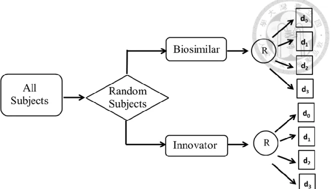
Design (a) in Figure 2.1 proposed by Liu and Chow (2010) consists of two dose- response trials, one for the biosimilar product and one for the innovator’s biological product, each with at least three dose levels with a placebo group. Eligible patients are first randomized into biosimilar or innovator groups. Within each group, patients are randomized again to receive one of the dose levels for the respective products. Well- defined product characteristics and primary efficacy endpoints are evaluated for all patients at their respective dose levels. Suppose that after a statistically significant relationship as represented by a simple linear regression equation can be established
between the well-defined product characteristics and the primary efficacy endpoint through dose levels for the innovator’s product, maybe after a suitable transformation.
For design (a) Liu and Chow (2010) suggest that the standard statistical method for analysis of parallel line assays can be used to construct the (1-2)100% confidence
interval for the relative potency in the following steps:
Step 1: Fit a linear regression equation to the primary efficacy endpoint with the group
mean of the product characteristics at each dose level as the independent variable separately for the biosimilar and innovator’s biological products. This may be done after
a suitable transformation.
Step 2: If the estimate of the slope of any one product is not significant at the pre-
15
defined level, then conclude that no simple relationship can be established between the product characteristic and primary endpoint and hence, a full clinical evaluation of the biosimilar product is required. Otherwise, go to Step 3.
Step 3: Test whether the two estimated simple linear regressions are parallel at the
predefined significance level. If the two estimated linear regressions are not parallel, then further clinical evaluation of the biosimilar product is warranted. Otherwise, proceed to
Step 4.
Step 4: Compute estimated relative potency and its corresponding (1-2)100%
confidence interval. If the (1-2)100% confidence interval for the relative potency is within the predefined margins (L, U), then equivalence in the product characteristic can be extrapolated to equivalence in the primary efficacy endpoint at the significance level.
Otherwise, further clinical investigation of the biosimilar product is needed.
Lin (2010), Chang (2011) and Lin et al. (2013) have applied the above procedure to continuous and binary responses. This thesis will consider the situation where the primary endpoint is a censored endpoint which follow an exponential distribution. Next section provides a brief review of survival analysis in terms of the exponential distribution with a right and random censored mechanism.
16
2.4 Survival Analysis
The following review is based on books by Lawless (2002) and Kleinbaum (1998).
Survival analysis involves the modeling of time to event data. The problem of analyzing time to event data arises in a number of applied fields, such as medicine, biology, public health, epidemiology, engineering, economics, and demography.
Although the statistical tools we shall present are applicable to all these disciplines, our focus is on applying the techniques to biology and medicine. The definition of lifetime includes a time scale and time origin, as well a specification of the event (e.g., failure or death) that determines lifetime. A common feature of these data sets is they contain censored. Censored data arises when an individual’s life length is known to occur only in a certain period of time. Possible censoring schemes are right censoring, where all that is known is that the individual is still alive at a given time, left censoring when all that is known is that the individual has experienced the event of interest prior to the start of the study, or interval censoring, where the only information is that the event occurs within some interval. Type I censoring occurs if an experiment has a set number of subjects or items and stops the experiment at a predetermined time, at which point any subjects remaining are right-censored. Type II censoring occurs if an experiment has a set number of subjects or items and stops the experiment when a predetermined number are observed
17
to have failed; the remaining subjects are then right-censored. Random (or non- informative) censoring is when each subject has a censoring time that is statistically independent of their failure time. The observed value is the minimum of the censoring and failure times; subjects whose failure time is greater than their censoring time are right- censored. In this thesis we only consider the right and random censoring mechanism.
We begin by considering the case of a single continuous lifetime variable, T.
Specifically, let T be a nonnegative random variable representing the lifetime of individuals in some population. All functions, unless stated otherwise, ate defined over the interval (0, ∞). Let f(t) denote the probability density function (p.d.f.) of T and let
the (cumulative) distribution function (c.d.f.) be
t
F t Pr T t
0 f x dx. (2.5) The probability of an individual surviving to time t is given by the survivor function( ) ( ) ( ) .
S t Pr T t
t f x dx (2.6) Note that S t
is a monotone decreasing continuous function with 0 S
1and
0) .
( t
S limS t A very important concept with lifetime distributions is the
hazard function h t
, denoted as
t
Pr t T<t t T t f t
h t lim .
t S t
(2.7)
The hazard function specifies the instantaneous rate of death or failure at time t, given that the individual survives up to t; h t
tis the approximate probability of death in18 , t)
[t t , given survival up to t.
The functions f t
, F t , S t and h t
give mathematically equivalentspecification of the distribution of T. It is easy to derive expressions for S t
and
f t in terms ofh t
; since f t
S t ,
implies that
h x d ln .
dx S x
(2.8)
Thus
0
0
lnS x | ,
t
t
h x dx (2.9)and since S
0 1, we find that
0
S t exp .
t
h x dx
(2.10)It is also useful to define the cumulative hazard function
0
H t ,
t
h x dx
(2.11)which is related to the survival function byS t
exp
H t
. If S( ) 0, then( ) 0
H .Finally, it follows immediately that
0
f t h t exp .
t
h x dx
(2.12)In clinical trials, individuals are followed longitudinally over time. The group of cohort of individuals in often, but not necessarily, randomly selected from a population of individuals who are at the time origin
t0
for the lifetime variable T. Limitations on the information collected may be imposed by time, cost, and other constraints.19
Termination of follow-up before an individual fails causes their lifetime to be right censored. A random censoring process that is often realistic is one in which each individual is assumed to have a life time T and censoring time C, with T and C independent continuous random variables, with survivor functions S t
and G t
,respectively.
All lifetimes and censoring times are assumed mutually independent, and it is assumed that G t
does not depend on any of the parameters of S t
. The data from observations on N individuals is assumed to consist of the pairs
y , δ , i i
i 1, N, whereyi Min T , C , δ
i i
i I T
i Ci
.The p.d.f. of
y , δi i
is easily obtained: if f t
and g t
are the p.d.f.’s forT
iand
C
i, then
i i
i i δi
i i 1 δiP y y, δ f y *G y g y *S y .
(2.13)
And thus the distribution of
y , δ , i i
i 1, N is
i i δi
i i 1 δi i=1f y *G y g y *S y .
N
(2.14)Since G t
and g t
do not involve any of the parameters in f t
, they can be neglected and the likelihood function taken to be
i δi
i 1 δi i=1f y S y
N
L
(2.15)In this study, we suppose that the lifetimes
T
i are independent and follow an20
exponential distribution with p.d.f. f t
λ exp λ t1
1
and the censoring timesC
iareindependent and follow an exponential distribution with p.d.f. g c
λ exp λ c2
2
. Let
i i i i i i
y Min T , C , δ I T C . I T
i Ci
is the indicator function. When the data isuncensored,
T
i C
i , I T
i Ci
1 . And when the data is uncensored,T >C
i i ,
i i
I T C 0. So the p.d.f. of
y , δi i
is
i i
δ 1 δ
1 2 i 1 2
(λ ) (λ ) exp y λ λ . (2.16)
The censored rate is calculated by integrating P
y , δi i 1
with respect toy
i, thenwe have
i i
i 1 1 2 1-1
i
1 2
i0 0
1 2
1 2
2
y , δ y (λ ) (λ ) exp y λ λ y λ
λ λ 1
λ .
1 λ
1
P d d
(2.17)
Let
λ λ
1 2 k
,the ratio of the two parameters. The censored rateCR1 (1k).
The expected value of lifetime is
i i i i i i i i
0 0
1 1-1 0 1-0
i 1 2 i 1 2 i i 1 2 i 1 2
0 0
1 2 1 2
1 2 1 2 1
2 2
1 2
1
y y , δ y y y , δ y
y (λ ) (λ ) exp y λ λ y y (λ ) (λ ) exp y λ λ
1 0
1 1
( )
y
λ λ ( )
1 1 1
(1 ) .
λ λ λ λ
λ λ λ λ λ λ (1 1 )
P d P d
d d
k
(2.18)
.
The hazard rate is reciprocal of the expected value of lifetime. So it is
λ (1 1 )
1 k
. If21
we assumed that censored rate is a fixed constant, then the hazard is affected by the only
parameter
λ
1.2.4 Log-hazard Linear Regression Model.
According to Liu and Chow (2010), group means of a well-defined product characteristic can be computed for each dose level for the biosimilar and innovator’s
product respectively. In this case, the variable of interest is positive and the log transformation is immediately applicable. In other words, the relationship between the log-hazard and the well-defined drug chacteristic can be modeled by a linear regression.
Thus the log-hazard linear regression model is given as:
iln λ α βx. (2.19)
where
x
i is dose level,
is the intercept and is the slope .Now we have the p.d.f. and the survival function for the lifetime of each individual base
on
and :
i i
i if y exp(α βx exp(-y exp(α ) βx)). (2.20)
i
i
i) i iS y Pr Yy exp( λy exp(-y exp(αβx )). (2.21)
To estimate the parameters, we need to use Method of Maximum Likelihood (MLE).
Let parameters vectorθ
,
T. Expressing the probabilities as a log-hazard c function of the covariate and the parameters yields the likelihood function from Eq.(2.15)22
i i
α βxi i i i
N δ 1 δ
i i i i i
i 1
N α βx δ e y
i 1
exp( )] exp(
L exp[α βx y α βx exp[ y α βx
{(e ) e }.
)]
(2.22)
It follows that the log likelihood is
α βxi i i i
i
N α βx δ e y
i 1
N N N
α βx
i i i i
i 1 i 1 i 1
lnL ln {(e ) e }
α δ β δ x y e .
θ
(2.23)
The score vector for the parameter is
[U(θ) , U(θ)α β]T.U θ (2.24)
where the score equation for the intercept is
N N
α βxi
α i i
i 1 i 1
U( ) lnL δ y e .
α
θ θ (2.25)
and the score equation for the regression coefficient is
N N
α βxi
β i i i i
i 1 i 1
U( ) lnL δ x x y e .
β
θ θ (2.26)
The expected information matrix
α αβαβ β
I( ) I( )
I I( ) I( )
θ θ
θ θ θ , where
i
N α βx
α α i
i 1
I( ) U( ) y e ,
α
θ θ (2.27)
i
N 2 α βx
β β i i
i 1
I( ) U( ) x y e ,
β
θ θ (2.28)
i
N α βx
αβ α i i
i 1
I( ) I( ) x y e .
β
θ θ (2.29)
23
Thus we have the expected information matrix
i i
i i
N N
α βx α βx
i i i
i 1 i 1
N N
α βx 2 α βx
i i i i
i 1 i 1
y e x y e
I .
x y e x y e
θ (2.30)
Note that each score equation involves the complete parameter vectorθ .The MLE is the vector ( ˆα, ˆβ)Tthat jointly satisfiesU
θ 0. Since the close-form solution do not exist, the solution must be obtained by an iterative procedure such as the Newton-Raphson algorithm. We review the Newton-Raphson algorithm in the next section.
To solve the MLE of α and β, we letU( )θ α 0, we have
N N
i i i
i 1 i 1
ˆ ˆ e
δ y xp(α βx ).
(2.31)i
N i 1 i
N βx
i 1 i ˆ
α ln δ .
y ˆ
e
(2.32)To solve MLE of β, we use Newton–Raphson method, given a function ƒ defined over β:
ii
N βx N
i i i i
i 1 i 1
N βx N
i i
i 1 i 1
x y e δ x
f β ,
y e δ
(2.33)and its derivative ƒ '
i ii i
N 2 βx N βx
i i i i 2
i 1 i 1
N βx N βx
i i
i 1 i 1
x y e x y e
f β ( ) .
y e y e
(2.34)The process is repeated as
24
n 1 n
β β f β .
f β
(2.35)
The MLE of β is obtained when the solutionf ˆ
βn 1 0by definition. The MLE of α isobtained by Eq.(2.32).
The observed information matrix ˆi θ
is obtained by replacing α and β by their MLEs αˆ andβˆ , respectively. Usingi θ
ˆ , the vector of parameter estimates can be solved using Newton-Raphson iterative procedure, or another algorithm. Wald tests and large sample confidence limits for the individual parameters, such as β , are readily computed using the large sample variance
1β
ˆ ˆ
ˆ β
V i θ obtained as the corresponding diagonal element of the estimated expected information, i θ
ˆ . The null and fitted likelihoods can also be used as the basis for a likelihood ratio test of the model.2.5 Newton-Raphson Method
Newton–Raphson method (or Newton's method) is a method for finding successively better approximations to the roots of a real-valued function. Assume that we have an initial guess as to the value of the parameter that is in the neighborhood” of the
desired solution
ˆ
. Taking a Taylor’s expansion of the estimatingU ˆ
about the starting value ˆ
0 , we have
ˆ ˆ(0) ˆ (0)
' ˆ(0)0U U ˆ U R, (2.36)
25
which implies that
(0) (0)
(0) (0)
' (0) (0)
ˆ ˆ
ˆ ˆ ˆ
ˆ .
ˆ
U U
U i
(2.37)
Because Newton’s method uses the Hessian at each step, this is equivalent to using the
observed information function. This equation is then applied iteratively until
ˆ
converges to a constant (the desired solution) using the sequence of equations
( ) ( )
( 1) ( ) ( )
' ( ) ( )
ˆ ˆ
ˆ ˆ ˆ
ˆ ˆ
i i
i i i
i i
U U
U i
(2.38)
for i = 0, 1, 2,…
For the case whereθ is a vector, the corresponding sequence of equations is
characterized as
( 1) ( ) ( ) -1 ( )
( ) ( ) -1 ( )
ˆ ˆ - ˆ ˆ
ˆ ˆ ˆ .
i i i i
i i i
θ θ U θ' U θ θ i θ U θ
(2.39)
The MLE is obtained when the solution
U θ ˆ
i1 0
by definition.The initial estimate is often the value expected under an appropriate null hypothesis or may be an estimate provided by a simple non-iterative moment estimator when such exists. Then the above expression is equivalent to determining the tangent to the log likelihood contour and projecting it to the abscissa to determine the next iterative estimate.
This process continues until the process converges.
The Newton-Raphson iteration is quadratic convergent in the sense that
U θ ˆ
26
approaches to 0 and it is a quadratic function of
ˆθ
. However, it is also sensitive to the choice of the initial or starting value. (Lachin, 2000)27
Figure 2.1: Design (a) for evaluation of extrapolation ability
28
Chapter 3 Proposed Methods
For the indirect assay with censored responses which follows an exponential distribution, we propose to use the log-hazard regressions to evaluation of the similarity
of biosimilar products.
Equation Chapter (Next) Section 1
3.1 Design
We use the design (a) which proposed by Liu and Chow (2010) and is introduced in section 2.3. If a similar linear relationship via the log-hazard linear regression can be also obtained for the biosimilar product and its corresponding linear regression equation is very close to the one for the innovator’s product, then equivalence in efficacy based on the primary efficacy endpoint may be claimed. Because the innovator’s product has been approved by the regulatory agencies due to its confirmed efficacy, therefore the objective of Design (a) is not to establish the efficacy of either biological products but to establish the similar patterns of the relationship between the well-defined product characteristics and primary efficacy endpoint for the two products. As a result, the sample size of Design (a) can be reduced significantly.
Similar to the chemical generic drug products, approval for the biosimilar drug products can be treated as the evaluation of post-approval changes. (ICH Q5E, 2005) and this post-approval change is the change of drug manufacturers. Therefore, as indicated by
29
Liu and Chow (2010), if the biosimilar drug products and the corresponding innovator’s biological products appear highly similar, and if in addition, based on the accumulated experience relevant information and data, minute differences observed in the product
characteristics are expected to have no clinically meaningful adverse effect of safety and efficacy profiles. Under this circumstance, biosimilar drug products and innovator’s
products can be considered similar. Therefore, except for the traditional pivotal bioequivalence study, no further data from pivotal phase III trials should be requested.
However, the above statement is based on a crucial assumption that at least one of the product characteristics is a validated and reliable predictor of the safety and efficacy profiles of the biological products. This is the reason why Chow and Liu (2010) porposed the Fundamental Biosimilarity Assumption (FBA) given in Section 1.3
For design (a), Liu and Chow (2010) suggest that the standard statistical method for analysis of parallel line assays can be used to construct the (1-2)100% confidence
interval for the relative potency in the 4 steps, which is provided in Section 2.3. We can use the similar approach to apply in log-hazard linear regression in the following steps when the primary endpoint as a censored random variable:
Step 1: Fit a linear log-hazard regression equation to the censored endpoint with the group
mean of the product characteristics at each dose level as the independent variable separately for the biosimilar and innovator’s biological products. It is easy to use Method
30
of Maximum Likelihood (MLE) to estimate the parameters, the intercept and the slope.
Step 2: If the estimate of the slope of any one product is not significant at the pre-
defined level, then conclude that no linear relationship based on log-hazard can be established between the product characteristic and the censored endpoint and hence, a full clinical evaluation of the biosimilar product is required. Otherwise, go to Step 3.
Step 3: Test whether the two estimated log-hazard linear regressions are parallel at the
predefined significance level. If the two estimated linear log-hazard linear regressions are not parallel, then further clinical evaluation of the biosimilar product is warranted.
Otherwise, proceed to Step 4.
Step 4: Compute estimated relative potency and its corresponding (1-2)100%
confidence interval. If the (1-2)100% confidence interval for the relative potency is within the predefined margins (L, U), then equivalence in the product characteristic can
be extrapolated to equivalence in the censored endpoint at the significance level.
Otherwise, further clinical investigation of the biosimilar product is needed.
3.2 The Procedure and Methods Based on Relative Potency of Product Characteristics
We can simplify the 4 steps to the follow steps:
Step 1: Fit log-hazard linear models.
Step 2: Test linearity of the two log-hazard regression models. (non-zero slopes)
31
Step 3: Test for parallelism lines of log-hazard regressions. (equivalence of slopes)
Step 4: Estimate relative potency and its confidence interval.
Step 1 is easy to implement by using Method of Maximum Likelihood (MLE) via the Newton–Raphson method to estimate the parameters, the intercept
and the slope
. In this setting, the innovative biological product is treated as the standardpreparation, and the biosimilar product is referred to as the test preparation. Let dependent variablefR
y (fT y ) be the probability of the clinical outcomes such as the death for the biosimilar and innovate products, respectively. Let independent variable (X) be the mean characteristics under different dose levels. Then the log-hazard linear regressionmodels of the innovative product and the biosimilar product are given respectively as
R R R
f y λ exp λ y , (3.1)
T T T
f y λ exp λ y . (3.2)
Therefore we can apply the Wald test to test the linearity of a log-hazard regression model.
The hypotheses of the non-zero slope for the innovator’s biological products (reference) and the biosimilar (test) are given respectively as
R 0
R
β 0
,
: 0
: . .
a β H v s H
(3.3)
T 0
T
β 0
.
: 0
: . .
a β H v s H
(3.4)