A New Method for Forecasting the TAIEX Based on High ˀOrder Fuzzy Logical Relationships
Chao-Dian Chen
1and Shyi-Ming Chen
1, 21Department of Computer Science and Information Engineering, National Taiwan University of Science and Technology, Taipei, Taiwan, R. O. C.
2Department of Computer Science and Information Engineering, Jinwen University of Science and Technology, Taipei County, Taiwan, R. O. C.
Abstract—In this paper, we present a new method to forecast the Taiwan Stock Exchange Capitalization Weighted Stock Index (TAIEX) based on highˀorder fuzzy logical relationships. First, the proposed method fuzzifies the historical data into fuzzy sets to form highˀorder fuzzy logical relationships. Then, it calculates the value of the variable between the subscripts of adjacent fuzzy sets appearing in the antecedents of highˀorder fuzzy logical relationships. Then, it lets the highˀorder fuzzy logical relationships having the same antecedent to form a highˀorder fuzzy logical relationship group. Finally, it chooses a highˀorder fuzzy logical relationship group to forecast the TAIEX. The proposed method gets a higher average forecasting accuracy rate than the existing methods to forecast the TAIEX.
Keywords—fuzzy sets, fuzzy time series, fuzzy forecasting, highˀorder fuzzy time series, highˀorder fuzzy logical relationships
I. INTRODUCTION
In [12], [13], and [14], Song and Chissom presented the concepts of fuzzy time series based on the fuzzy set theory [21], where the values of fuzzy time series are represented by fuzzy sets. In recent years, some methods have been presented to handle forecasting problems based on fuzzy time series, such as enrollments forecasting [1], [2], [3], [4], [13], [14], [16], [20], temperature prediction [5], [11], [15], stock index forecasting [6], [8], [9], [10], [15], [17], [18], [19], [21], …, etc.
In this paper, we present a new method to forecast the Taiwan Stock Exchange Capitalization Weighted Stock Index (TAIEX) based on highˀorder fuzzy logical relationships groups. First, the proposed method fuzzifies the historical data into fuzzy sets to form highˀorder fuzzy logical relationships.
Then, it calculates the value of the variable between the subscripts of adjacent fuzzy sets appearing in the antecedents of highˀorder fuzzy logical relationships. Then, it lets the highˀ order fuzzy logical relationships having the same antecedent to form a highˀorder fuzzy logical relationship group. Finally, it chooses a highˀorder fuzzy logical relationship group to forecast the TAIEX. The proposed method gets a higher average forecasting accuracy rate than Chen’s method [1], Chen and Wang’s method [6], Huarng’s method [8], Huarng and Yu’s method [9], and Yu’s method [18] for forecasting the TAIEX.
The rest of this paper is organized as follows. In Section II, we briefly review the concept of fuzzy time series from [12], [13] and [14]. In Section III, we present a new method to forecast the TAIEX based on highˀorder fuzzy logical relationships. In Section IV, we make a comparison of the forecasting result of the proposed method with the existing methods. The conclusions are discussed in Section V.
II. PRELIMINARIES
In [12], [13] and [14], Song and Chissom presented the concepts of fuzzy time series based on the fuzzy set theory [21], where the values in a fuzzy time series are represented by fuzzy sets. Let U be the universe of discourse, where U= {u1, u2, …, un}. A fuzzy set Ai in the universe of discourse U is defined as follows:
Ai= fAi(u1)/u1+ fAi(u2)/u2+ …+ fAi(un)/un,
where fAi is the membership function of the fuzzy set Ai, fAi:U→[0,1], fAi(uj) is the degree of membership of ujbelonging to the fuzzy set Ai, fAi(uj)∈[0,1] and 1 ≤ j ≤ n.
Definition 2.1 [12]: Let Y(t) (t = …, 0, 1, 2, …) be the universe of discourse and be a subset of R. Assume that fi(t) (i= 1, 2, …) are defined in the universe of discourse Y(t), and assume that F(t) is a collection of fi(t) (i= 1, 2, …), then F(t) is called a fuzzy time series of Y(t) (t= …, 0, 1, 2, …).
If there exists a fuzzy relation R(t−1, t), such that F(t) = F(t−1) D R(t−1, t), where the symbol “D” represents the max- min composition operator, then F(t) is called caused by F(t−1) [12].
Definition 2.2: Let F(t−1) = Ai and let F(t)= Aj, where Ai
and Aj are fuzzy sets, then the fuzzy logical relationship (FLR) between F(t−1) and F(t) can be denoted by Ai→ Aj, where Ai and Aj are called the leftˀhand side (LHS) and the rightˀhand side (RHS) of the fuzzy logical relationship, respectively.
Fuzzy logical relationships having the same left hand side can be grouped into a fuzzy logical relationship group (FLRG) [1]. For example, assume that the following fuzzy logical relationships exist:
Ai→ Aja, Ai→ Ajb,
#
Ai→ Ajm, Proceedings of the 2009 IEEE International Conference on Systems, Man, and Cybernetics
San Antonio, TX, USA - October 2009
then these fuzzy logical relationships can be grouped into a fuzzy logical relationship group, shown as follows:
Ai→ Aja, Ajb, …, Ajm.
Let F(t) be a fuzzy time series. If F(t) is caused by F(t−1), F(t−2), …, and F(t−n), then the fuzzy logical relationship between them can be represented by the “nthˀorder fuzzy logical relationship”[2], shown as follows:
F(t−n), …, F(t−2), F(t−1) → F(t).
If F(t−n) = Ain, …, F(t−2) = Ai2, F(t−1) = Ai1, F(t)= Aj, where Ain, …, Ai2, Ai1, Aj are fuzzy sets, then the nthˀorder fuzzy logical relationship can be represented by
Ain, …, Ai2, Ai1→ Aj,
where Ain, …, Ai2, and Ai1 are called the antecedent fuzzy sets of the nthˀorder fuzzy logical relationship; “Ain, …, Ai2, Ai1” and “Aj” are called the leftˀhand side and the rightˀhand side of the nthˀorder fuzzy logical relationship, respectively.
If there exist the nthˀorder fuzzy logical relationships having the same left hand side, shown as follows:
Ain, …, Ai2, Ai1→ Aja, Ain, …, Ai2, Ai1→ Ajb,
#
Ain, …, Ai2, Ai1→ Ajm,
then these nthˀorder fuzzy logical relationships form a nthˀ order fuzzy logical relationships group, shown as follows:
Ain, Ai(n−1), …, Ai1→ Aja, Ajb, …, Ajm.
III. A NEW METHOD FOR FORECASTING THE TAIEX BASED ONHIGHˀORDER FUZZY LOGICAL RELATIONSHIPS In this section, we present a new method for forecasting the TAIEX based on highˀorder fuzzy logical relationships. We divide the historical data of the TAIEX into two parts, where one part is used as the training data set and the other as the testing data set. The training data set and the testing data set of the TAIEX of every year from 1991 to 1999 are shown in Table I [7], respectively. The proposed method for forecasting the TAIEX based on highˀorder fuzzy logical relationships is shown as follows:
Step 1: Define the universe of discourse U, U = [Dmin−D1, Dmax+D2] into intervals of equal length, where Dmin and Dmax are the minimum value and the maximum value of the historical data, respectively, and D1 and D2 are two proper positive real values to divide the universe of discourse U into n intervals u1, u2, …, un of equal length. For example from Table II, we can see that the minimum and the maximum stock indices of the year 1999 are 5474.79 and 8608.91, respectively.
If we let D1 = 74.79 and D2 = 91.09, then the universe of discourse U = [5400, 8700]. Let the length of each interval in the universe of discourse U be 25. Then, the universe of discourse U can be divided into 132 intervals, which are defined as follows:
ui= [5400 + (i − 1) × 25, 5400 + (i) × 25], (1) where i= 1, 2, …, 132.
TABLE I. TRAINING DATA SET AND TESTING DATA SET OF THE TAIEX
FROM1991 TO 1999 [7]
Year 1991 1992 1993 1994 1995 1996 1997 1998 1999 Training
data set 1/1~
10/30 1/4~
10/30 1/5~
10/30 1/5~
10/29 1/5~
10/30 1/4~
10/30 1/4~
10/30 1/3~
10/31 1/5~
10/30 Testing
data set 11/1~
12/28 11/2~
12/29 11/2~
12/31 11/1~
12/31 11/1~
12/30 11/1~
12/31 11/3~
12/31 11/2~
12/31 11/1~
12/28
TABLE II. HISTORICAL TRAINING DATA OF THE TAIEX OF 1999 [7]
Date TAIEX 1999/1/5 6152.43 1999/1/6 6199.91 1999/1/7 6404.31 1999/1/8 6421.75
# #
1999/10/28 7681.85 1999/10/29 7706.67 1999/10/30 7854.85
TABLE III. HISTORICAL TESTING DATA OF THE TAIEX OF 1999 [7]
Date TAIEX 1999/11/1 7814.89 1999/11/2 7721.59 1999/11/3 7580.09 1999/11/4 7469.23
# #
1999/12/24 8219.45 1999/12/27 8415.07 1999/12/28 8448.84
Step 2: Define the linguistic term Ai represented by fuzzy sets, shown as follows:
A1= 1/u1 + 0.5/u2 + 0/u3 + 0/u4 +…+ 0/un−1 + 0/un, A2= 0.5/u1 + 1/u2 + 0.5/u3 + 0/u4 +…+ 0/un−1 + 0/un, A3= 0/u1 + 0.5/u2 + 1/u3 + 0.5/u4 +…+ 0/un−1 + 0/un,
#
An−1= 0/u1 + 0/u2 + 0/u3 + 0/u4 +…+ 1/un−1 + 0.5/un, An= 0/u1 + 0/u2 + 0/u3 + 0/u4 +…+ 0.5/un−1 + 1/un.
where A1, A2, …, and An are linguistic terms represented by fuzzy sets. For example, based on the obtained 132 intervals, we define the linguistic terms A1, A2, …, and A132, shown as follows:
A1= 1/u1 + 0.5/u2 + 0/u3 + 0/u4 + …+ 0/u131 + 0/u132, A2= 0.5/u1 + 1/u2 + 0.5/u3 + 0/u4 + …+ 0/u131 + 0/u132, A3= 0/u1 + 0.5/u2 + 1/u3 + 0.5/u4 + …+ 0/u131 + 0/u132,
#
A131 = 0/u1 + 0/u2 + 0/u3 + 0/u4 + …+ 1/u131 + 0.5/u132, A132 = 0/u1 + 0/u2 + 0/u3 + 0/u4 + …+ 0.5/u131 + 1/u132. Step 3: Fuzzify each historical datum into a fuzzy set defined in Step 2. If the historical datum belongs to ui and the maximum membership value of Ai occurs at ui, then the historical datum is fuzzified into Ai, where 1 ≤ i ≤ n. For
example, the TAIEX of 1999/1/5 shown in Table II is 6152.43, which is fuzzified into A31, as shown in Table IV. In the same way, the TAIEX of 1999/1/6 shown in Table II is 6199.91, which is fuzzified to A32, as shown in Table IV. Table IV and Table V show the fuzzified TAIEX of the training data set and the testing data set of 1999, respectively.
TABLE IV. FUZZIFY TAIEX OF THE TRAINING DATA SET
Date Fuzzy Set
1999/1/5 A31
1999/1/6 A32
1999/1/7 A41
1999/1/8 A41
# #
1999/10/28 A92
1999/10/29 A93
1999/10/30 A99
TABLE V. FUZZIFIED TAIEX OF THE TESTING DATA SET
Date Fuzzy Set
1999/11/1 A97
1999/11/2 A93
1999/11/3 A88
1999/11/4 A83
# #
1999/12/24 A113
1999/12/27 A121
1999/12/28 A122
Step 4: Construct the nthˀorder fuzzy logical relationships from the fuzzified TAIEX of the training data set. For example, from Table IV, we can see that the fuzzified TAIEX of 1999/1/5 is A31, the fuzzified TAIEX of 1999/1/6 is A32, and the fuzzified TAIEX of 1999/1/7 is A41. Thus, we can get the following secondˀorder fuzzy logical relationship:
A31,A32→ A41.
From Table IV, we also can see that the fuzzified TAIEX of 1999/1/6 is A32, the fuzzified TAIEX of 1999/1/7 is A41, and the fuzzified TAIEX of 1999/1/8 is A41. Thus, we can get the following secondˀorder fuzzy logical relationship:
A32,A41→ A41.
In the same way, we can get the other fuzzy logical relationships from the fuzzified TAIEX of the training data set shown in Table IV, as shown in Table VI.
Step 5: Transform each nthˀorder fuzzy logical relationship
“AX1, AX2, AX3, …, AXj, …, AXn→ AXr” into the following form:
AX1, AX1+V(X1), AX1+V(X1)+V(X2), …, AX1+V(X1)+V(X2)+…+V(Xi), …, AX1+V(X1)+V(X2)+…+V(Xi)+…+V(Xm) → AX1+V(X1)+V(X2)+…+V(Xi)+…+V(Xm)+V(Xn), where V(X1), V(X2), …, and V(Xn) are integers. For example, if the secondˀorder fuzzy logical relationship is “A31, A32 → A41”, then we can transform it into: “AX1, AX1+V(X1) → AX1+V(X1)+V(X2)”, where the subscripts X1, X2, and X3 of the fuzzy sets A31, A32, and A41 are 31, 32, and 41, respectively, i.e; X1= 31, X2= 32 and X3 = 41. Thus, we can get V(X1) = X2 − X1 = 32 −31 = 1 and V(X2) = X3 − (X1+V(X1)) = X3 − X2 = 41 −32
= 9. Therefore, the secondˀorder fuzzy logical relationship
“A31,A32 → A41” is represented as: “A31, A31+1 → A31+1+9”.
Moreover, we can see that the secondˀorder fuzzy logical
relationship “A32, A41→ A41” is represented as: “A32, A32+9→ A32+9+0”. In the same way, we can transform the secondˀorder fuzzy logical relationships shown in Table VI into Table VII.
TABLE VI. SECONDˀORDERFUZZYLOGICAL RELATIONSHIPS
Date Fuzzy Logical
Relationships 1999/1/5,1999/1/6 → 1999/1/7 A31, A32→ A41
1999/1/6,1999/1/7→ 1999/1/8 A32, A41→ A41
1999/1/7,1999/1/8 → 1999/1/11 A41, A41→ A41
1999/1/8,1999/1/11 → 1999/1/12 A41, A41→ A39
# #
1999/10/26,1999/10/27 → 1999/10/28 A93, A93→ A92
1999/10/27,1999/10/28 → 1999/10/29 A93, A92→ A93
1999/10/28,1999/10/29 → 1999/10/30 A92, A93→ A99
TABLE VII. TRANSFORMED FUZZYVARIABLE LOGICAL RELATIONSHIPS
Date Fuzzy Variable Logical Relationships 1999/1/5,1999/1/6 → 1999/1/7 A31, A31+1→ A31+1+9
1999/1/6,1999/1/7→ 1999/1/8 A32, A32+9→ A32+9+0
1999/1/7,1999/1/8 → 1999/1/11 A41, A41+0→ A41+0+0
1999/1/8,1999/1/11 → 1999/1/12 A41, A41+0→ A41+0−2
# #
1999/10/26,1999/10/27 → 1999/10/28 A93, A93+0→ A93+0−1
1999/10/27,1999/10/28 → 1999/10/29 A93, A93−1→ A93−1+1
1999/10/28,1999/10/29 → 1999/10/30 A92, A92+1→ A92+1+6
Step 6: Let the transformed nthˀorder fuzzy logical relationships obtained in Step 5 having the same leftˀhand side form a nthˀorder fuzzy logical relationship group. For example, let us consider the following transformed thirdˀorder fuzzy logical relationships: “Aa1, Aa1+V(a1), Aa1+V(a1)+V(a2) → Aa1+V(a1)+V(a2)+V(a3)”, “Ab1, Ab1+V(b1), Ab1+V(b1)+V(b2) → Ab1+V(b1)+V(b2)+V(b3)”, …, and “Ak1, Ak1+V(k1), Ak1+V(k1)+V(k2) → Ak1+V(k1)+V(k2)+V(k3)”, where V(a1)= V(b1) = … = V(k1) and V(a2)
= V(b2) = … = V(k2), then these thirdˀorder fuzzy logical relationships can be grouped into a transformed thirdˀorder fuzzy logical relationships group, shown as follows:
Aa1, Aa1+V(a1), Aa1+V(a1)+V(a2)→ Aa1+V(a1)+V(a2)+V(a3), Ab1, Ab1+V(b1), Ab1+V(b1)+V(b2)→ Ab1+V(b1)+V(b2)+V(b3),
#
Ak1, Ak1+V(k1), Ak1+V(k1)+V(k2)→ Ak1+V(k1)+V(k2)+V(k3).
Moreover, this transformed thirdˀorder fuzzy logical relationships group can be represented as:
AX, AX+V(y1), AX+V(y1)+V(y2) → AX+V(y1)+V(y2)+V(a3), AX+V(y1)+V(y2)+V(b3), …, AX+V(y1)+V(y2) +V(k3). where X= a1, b1, …, k1, V(y1)= V(a1) = V(b1) = … = V(k1) and V(y2) = V(a2) = V(b2) = … = V(k2). For example, let us consider the secondˀ order fuzzy logical relationships “A31, A31+1→ A31+1+9”, “A43, A43+1→ A43+1−4”, and “A37, A37+1 → A37+1−4” shown in Table VII, where their transformed secondˀorder fuzzy logical relationships are “Ax, Ax+1→ Ax+1+9”, “Ax, Ax+1→ Ax+1−4”, and
“Ax, Ax+1 → Ax+1−4”, respectively. Because these transformed secondˀorder fuzzy logical relationship have the same leftˀhand
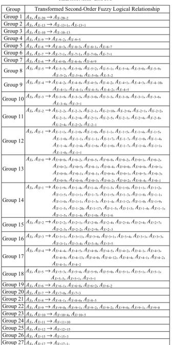
side “AX, AX+1”, we can group them into a transformed secondˀ order fuzzy logical relationship group “AX, AX+1 → AX+1+9, AX+1−4, AX+1−4”. Table VIII shows the transformed secondˀorder fuzzy logical relationship groups derived from Table VII.
TABLE VIII. TRANSFORMED SECONDˀORDER FUZZY LOGICAL
RELATIONSHIP GROUPS
Group Transformed SecondˀOrder Fuzzy Logical Relationship Group 1 AX, AX−20→ AX−20−2
Group 2 AX, AX−13→ AX−13+1, AX−13+1 Group 3 AX, AX−10→ AX−10−13
Group 4 AX, AX−9→ AX−9−2, AX−9+5
Group 5 AX, AX−8→ AX−8+3, AX−8+3, AX−8+1, AX−8−7
Group 6 AX, AX−7→ AX−7+1, AX−7+1, AX−7+0, AX−7+1
Group 7 AX, AX−6→ AX−6+0, AX−6−6, AX−6+9
Group 8 AX, AX−5→ AX−5−5, AX−5+0, AX−5+2, AX−5−1, AX−5+4, AX−5+0, AX−5−9, AX−5+2, AX−5+6, AX−5+0, AX−5−2
Group 9 AX, AX−4→ AX−4−2, AX−4−8, AX−4+3, AX−4−2, AX−4+1, AX−4+3, AX−4−10, AX−4+1, AX−4−1, AX−4−5, AX−4−2, AX−4+5
Group 10 AX, AX−3→ AX−3+9, AX−3−3, AX−3+0, AX−3−3, AX−3−8, AX−3+1, AX−3−6, AX−3−6, AX−3+1
Group 11
AX, AX−2→ AX−2−2, AX−2−3, AX−2−1, AX−2+10, AX−2+6, AX−2+1, AX−2+2, AX−2−1, AX−2+4, AX−2+1, AX−2−5, AX−2−1, AX−2+4, AX−2−8, AX−2+4, AX−2+2, AX−2−1
Group 12
AX, AX−1→ AX−1+1, AX−1+0, AX−1+0, AX−1−1, AX−1+5, AX−1+4, AX−1+5, AX−1+0, AX−1−1, AX−1−1, AX−1+7, AX−1−7, AX−1+0, AX−1−4, AX−1−4, AX−1+4, AX−1+6, AX−1+0, AX−1−7, AX−1+4, AX−1+1, AX−1+0, AX−1+1
Group 13
AX, AX+0→ AX+0+0, AX+0−2, AX+0−5, AX+0−9, AX+0−2, AX+0+1, AX+0−2, AX+0+2, AX+0+5, AX+0−1, AX+0−4, AX+0+0, AX+0+0, AX+0+1, AX+0+0, AX+0−1, AX+0−1, AX+0+4, AX+0+1, AX+0+5, AX+0−3, AX+0+9, AX+0+4, AX+0+3, AX+0−2, AX+0+2, AX+0−4, AX+0−1
Group 14
AX, AX+1→ AX+1+9, AX+1−4, AX+1−4, AX+1−3, AX+1+0, AX+1+1, AX+1+2, AX+1+5, AX+1+1, AX+1−7, AX+1+5, AX+1−3, AX+1+8, AX+1−1, AX+1+0, AX+1+1, AX+1−3, AX+1−4, AX+1+2, AX+1+0, AX+1+9, AX+1−5, AX+1−20, AX+1+17, AX+1−5, AX+1+3, AX+1−4, AX+1−1, AX+1−5, AX+1−4, AX+1+0, AX+1+6
Group 15 AX, AX+2→ AX+2+2, AX+2+1, AX+2+0, AX+2−4, AX+2+4, AX+2+4, AX+2+7, AX+2−3, AX+2−2, AX+2+9, AX+2−3
Group 16 AX, AX+3→ AX+3+1, AX+3+11, AX+3+4, AX+3+1, AX+3+4, AX+3+1, AX+3+3, AX+3+1, AX+3−4, AX+3−8, AX+3+5
Group 17
AX, AX+4→ AX+4−4, AX+4+5, AX+4+0, AX+4−5, AX+4+2, AX+4−1, AX+4+3, AX+4+8, AX+4−13, AX+4+0, AX+4+12, AX+4+4, AX+4−1, AX+4−2, AX+4−1, AX+4−2
Group 18 AX, AX+5→ AX+5+3, AX+5+4, AX+5+9, AX+5+0, AX+5+1, AX+5+1, AX+5−1, AX+5−5, AX+5+1, AX+5+1
Group 19 AX, AX+6→ AX+6−1, AX+6+8, AX+6+2, AX+6−2
Group 20 AX, AX+7→ AX+7+0, AX+7+3
Group 21 AX, AX+8→ AX+8−1, AX+8+6, AX+8−5
Group 22 AX, AX+9→ AX+9+0, AX+9+1, AX+9−2, AX+9−2, AX+9+0, AX+9−1, AX+9+0
Group 23 AX, AX+10→ AX+10+4, AX+10−5
Group 24 AX, AX+11→ AX+11+10
Group 25 AX, AX+12→ AX+12+15 Group 26 AX, AX+15→ AX+15+3
Group 27 AX, AX+17→ AX+17−1.
Step 7: Choose a transformed nthˀorder fuzzy logical relationship group for prediction. Assume that F(t−n) = Ain, F(t−(n−1)) = Ai(n−1), …, F(t−2) = Ai2, and F(t−1) = Ai1, and assume that we want to predict F(t), where Ai1, Ai2, …, and Ain
are fuzzy sets. Based on the transformed nthˀorder fuzzy logical relationship groups obtained in Step 6, choose the corresponding transformed nthˀorder fuzzy logical relationship
group for prediction. If the chosen transformed nthˀorder fuzzy logical relationship group is: “AX, AX+V(y1), …, AX+V(y1)+V(y2)+…+V(y(n−1)) → AX+V(y1)+…+V(y(n−1))+V(an), AX+V(y1)+…+V(y(n−1))+V(bn), …, AX+V(y1)+…+V( y(n−1))+V(kn)”, where Ain= AX, Ai(n−1) = AX+V(y1), …, Ai1 = AX+V(y1)+ V(y2)+…+V(y(n−1)), then replace X by the subscript in of the fuzzy set Ain to get the derived fuzzy sets Ain+V(y1)+…+V(y(n−1))+V(an), Ain+V(y1)+…+V(y(n−1))+V(bn), …, and Ain+V(y1)+…+V(y(n−1))+V(kn) for prediction. Let Aj1 = Ain+V(y1)+…+V(y(n−1))+V(an), let Aj2 = Ain+V(y1)+…+V(y(n−1))+V(bn), …, and let Ajk = Ain+V(y1)+…+V(y(n−1))+V(kn). Then, the forecasted value FV of day t is calculated as follows:
k m FV
k i¦ ji
= =1 , (2) where the maximum membership values of Aj1, Aj2, …, and Ajk, occur at the intervals uj1, uj2, …, and ujk, respectively, and mj1, mj2, …, and mjk are the midpoints of uj1, uj2,…, and ujk, respectively. For example, assume that we want to forecast the TAIEX of 1999/11/3 by the secondˀorder fuzzy logical relationships. From Table V, we can see that the fuzzified TAIEX of 1999/11/1 and 1999/11/2 are A97 and A93, respectively. Therefore, we can see that A97 and A93 can be transformed into Ax and Ax−4, respectively, where X = 97. Based on Table VIII, we choose Group 9 of the transformed secondˀ order fuzzy logical relationships group for prediction, i.e., AX, AX−4 → AX−4−2, AX−4−8, AX−4+3, AX−4−2, AX−4+1, AX−4+3, AX−4−10, AX−4+1, AX−4−1, AX−4−5, AX−4−2, AX−4+5. By letting X be 97, we can see that AX−4−2, AX−4−8, AX−4+3, AX−4−2, AX−4+1, AX−4+3, AX−4−10, AX−4+1, AX−4−1, AX−4−5, AX−4−2, and AX−4+5 become A91, A85, A96, A91, A94, A96, A83, A94, A92, A88, A91 and A98, respectively. Then, the forecasted TAIEX of 1999/11/3 is equal to the average of the midpoints u91, u85, u96, u91, u94, u96, u83, u94, u92, u88, u91 and u98, where the maximum membership values of the fuzzy sets A91, A85, A96, A91, A94, A96, A83, A94, A92, A88, A91 and A98 occur at u91, u85, u96, u91, u94, u96, u83, u94, u92, u88, u91 and u98, respectively. From Eq. (1), we can see that the midpoints of the intervals u91, u85, u96, u91, u94, u96, u83, u94, u92, u88, u91 and u98
are 7662.5, 7512.5, 7787.5, 7662.5, 7737.5, 7787.5, 7462.5, 7737.5, 7687.5, 7587.5, 7662.5 and 7837.5, respectively. Thus, based on Eq. (2), the forecasted TAIEX of 1999/11/3 is calculated as follows:
7677.08.
12
7837.5 7662.5 7587.5 7687.5 7737.5 7462.5 7787.5 7737.5 7662.5 7787.5 7512.5 7662.5
+ = + + + + + + + + + +
That is, the forecasted TAIEX of 1999/11/3 is 7677.08.
IV. EXPERIMENTAL RESULTS
In this section, we apply the proposed method for forecasting the TAIEX from 1991 to 1999 with different lengths of intervals. We evaluate the performance of the proposed method using the root mean square error (RMSE), which is defined as follows:
n
value actual value forecasted RMSE
n
i¦ i− i
= =1
)2 (
, (3) where n denotes the number of dates needed to be forecasted, forecasted valuei denotes the forecasted value of day i, actual
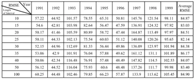
valuei denotes the actual value of day i and 1 ≤ i ≤ n. Table IX makes a comparison of the RMSE and the average RMSE of the proposed method to forecast the TAIEX for different lengths of intervals.ʳ From Table IX, we can see that when the length of interval is 25, the proposed method gets the smallest average RMSE. In Table X, we make a comparison of the RMSE and the average RMSE of the proposed method with Chen’s method [1], Chen and Wang’s method [6], Huarng’s method [8], Huarng and Yu’s method [9], and Yu’s method [18]. From Table X, we can see that the proposed method gets the smallest average RMSE comparing to Chen’s method [1], Chen and Wang’s method [6], Huarng’s method [8], Huarng and Yu’s method [9], and Yu’s method [18]. It means that the proposed method gets a higher average forecasting accuracy rate than Chen’s method [1], Chen and Wang’s method [6], Huarng’s method [8], Huarng and Yu’s method [9], and Yu’s method [18] to forecast the TAIEX.
TABLE IX. A COMPARISON OF THE RMSES AND THE AVERAGE RMSE OF THEPROPOSED METHOD FOR DIFFERENT LENGTHS OF INTERVALS
1991 1992 1993 1994 1995 1996 1997 1998 1999 Average RMSE 10 57.22 44.92 101.57 78.55 65.31 50.81 145.76 121.54 98.11 84.87 15 54.6 42.81 103.98 82.64 56.47 47.59 136.91 124.32 97.92 83.03 20 50.17 41.46 105.59 80.89 58.72 47.44 164.87 113.49 97.97 84.51 25 50.11 44.33 102.13 75.54 60.03 51.12 140.08 120.26 95.65 82.14 30 52.15 44.96 112.69 81.33 56.44 49.86 136.09 123.97 101.94 84.38 35 53.06 42.9 101.91 76.04 57.88 49.62 161.12 131.1 101.89 86.17 40 50.06 42.34 116.48 76.91 57.48 48.49 147.82 114.5 102.53 84.07 50 56.12 44.52 116.04 75.93 60.6 48.48 137.26 111.7 99.98 83.40 100 60.25 44.48 102.46 79.85 66.23 57.87 133.9 113.62 105.45 84.90
TABLE X. A COMPARISON OF THE RMSES AND THE AVERAGE RMSE FOR
DIFFERENT METHODS
1991 1992 1993 1994 1995 1996 1997 1998 1999 Average RMSE Chen’s Method
[1] 80 60 110 112 79 54 148 167 149 107
Chen and Wang’s
Method [6] 42.89 43.48 103.37 89.81 52.2 52.83 140.75 116.88 104.88 83.01 Huarng’s Method
[8] Based on Average-Based Length Interval
79.4 59.9 105.2 132.4 78.6 52.1 148.8 159.3 159.1 108.3
Huarng’s Method [8] Based on Distribution- Based Length
Interval
80.2 60.3 110 111.7 78.6 54.2 148.0 167.3 148.7 106.5
Huarng and Yu’s
Method [9] 54.7 61.1 117.9 88.7 64.1 52.1 135.9 136.2 131.9 93.1 Yu’s Method
[18] 61 67 105 135 70 54 133 151 142 102
The Proposed
Method 50.11 44.33 102.13 75.54 60.03 51.52 140.08 120.26 95.65 82.14
V. CONCLUSIONS
In this paper, we have presented a new method for forecasting the Taiwan Stock Exchange Capitalization Weighted Stock Index (TAIEX) based on highˀorder fuzzy logical relationships. From Table X, we can see that the proposed method gets the smallest average RMSE comparing to Chen’s method [1], Chen and Wang’s method [6], Huarng’s method [8], Huarng and Yu’s method [9], and Yu’s method [18] for forecasting the TAIEX. That is, the proposed method gets a higher average forecasting accuracy rate than Chen’s method [1], Chen and Wang’s method [6], Huarng’s method [8], Huarng and Yu’s method [9] and Yu’s method [18] forʳ forecasting the TAIEX.
ACKNOWLEDGMENT
This work is supported in part by the National Science Council, Republic of China, under Grant NSC 97-2221-E-011- 107-MY3.
REFERENCES
[1] S. M. Chen, “Forecasting enrollments based on fuzzy time series,”
Fuzzy Sets and Systems, vol. 81, no. 3, pp. 311-319, 1996.
[2] S. M. Chen, “Forecasting enrollments based on high-order fuzzy time series,” Cybernetics and Systems, vol. 33, no. 1, pp. 1-16, 2002.
[3] S. M. Chen and N. Y. Chung, “Forecasting enrollments using high- order fuzzy time series and genetic algorithm,” International Journal of Intelligent Systems, vol. 21, no. 5, pp. 485-501, 2006.
[4] S. M. Chen and C. C. Hsu, “A new method to forecast enrollments using fuzzy time series,” International Journal of Applied Science and Engineering, vol. 2, no. 3, pp. 234-244, 2004.
[5] S. M. Chen and J. R. Hwang, “Temperature prediction using fuzzy time series,” IEEE Transactions on Systems, Man, and Cybernetics-Part B:
Cybernetics, vol. 30, no. 2, pp. 263-275, 2000.
[6] S. M. Chen and N. Y. Wang, “Handling forecasting problems based on high-order fuzzy time series and fuzzy-trend logical relationships,”
Proceedings of the 2008 Workshop on Consumer Electronics, Taipei County, Taiwan, Republic of China, pp. 759-764, 2008.
[7] Taiwan Stock Exchange (http://www.twse.com.tw/en/products/indices/
tsec/taiex.php).
[8] K. Huarng, “Effective lengths of intervals to improve forecasting in fuzzy time series,” Fuzzy Sets and Systems, vol. 123, no. 3, pp. 387- 394, 2001.
[9] K. Huarng and H. K. Yu, “Ratio-based lengths of intervals to improve fuzzy time series forecasting,” IEEE Transactions on Systems, Man, and, Cybernetics-Part B: Cybernetics, vol. 36, no. 2, pp. 328-340, 2006.
[10] K. Huarng, H. K. Yu, and Y. W. Hsu “A multivariate heuristic model for fuzzy time-series forecasting,” IEEE Transactions on Systems, Man, and, Cybernetics Part-B: Cybernetics, vol. 37, no. 4, pp. 836-846, 2007.
[11] L. W. Lee, L. H. Wang, S. M. Chen, and Y. H. Leu, “Handling forecasting problems based on two-factors high-order fuzzy time series,” IEEE Transactions on Fuzzy Systems, vol. 14 , no. 3, pp. 468- 477, 2006.
[12] Q. Song and B. S. Chissom, “Fuzzy time series and its model,” Fuzzy Sets and Systems, vol. 54, no. 3, pp. 269-277, 1993.
[13] Q. Song and B. S. Chissom, “Forecasting enrollments with fuzzy time series - Part I,” Fuzzy Sets and Systems, vol. 54, no. 1, pp. 1-9, 1993.
[14] Q. Song and B. S. Chissom, “Forecasting enrollments with fuzzy time series - Part II,” Fuzzy Sets and Systems, vol. 62, no. 1, pp. 1-8, 1994.
[15] N. Y. Wang and S. M. Chen, “Temperature prediction and TAIFEX forecasting based on automatic clustering techniques and two-factors high-order fuzzy time series,” Expert Systems with Applications, vol.
36, no. 2, pp. 2143-2154, March 2009.
[16] N. Y. Wang, S. M. Chen, and J. S. Pan, “Forecasting enrollments based on automatic clustering techniques and fuzzy time series,” Proceedings of the 12th Conference on Artificial Intelligence and Applications, Yunlin, Taiwan, Republic of China.
[17] H. K. Yu, “A refined fuzzy time-series model for forecasting,” Physica A, vol. 346, no. 3-4, pp. 657–681, 2004.
[18] H. K. Yu, “Weighted fuzzy time-series models for TAIEX forecasting,” Physica A, vol. 349, no. 3-4, pp. 609–624, 2004.
[19] H. K. Yu and K. H. Huarng, “A bivariate fuzzy time series model to forecast the TAIEX,” Expert Systems with Applications, vo1. 34, no. 4, pp. 2945-2952, 2008.
[20] I. H. Kuo, S. J. Horng, T. W. Kao, T. L. Lin, C. L. Lee, and Y. Pan,
“An improved method for forecasting enrollments based on fuzzy time series and particle swarm optimization,” Expert Systems with Applications, vo1. 36, no. 3, pp. 6108-6117, 2009.
[21] H. J. Teoh, T. L. Chen, C. H. Cheng, and H. H. Chu, “A hybrid multi- order fuzzy time series for forecasting stock markets,” Expert Systems with Applications, vo1. 36, no. 4, pp. 7888-7897, 2009.
[22] L. A. Zadeh, “Fuzzy sets,” Information and Control, vol. 8, pp. 338- 353, 1965.
RMSE Length of Interval
Year
RMSE Method
Year